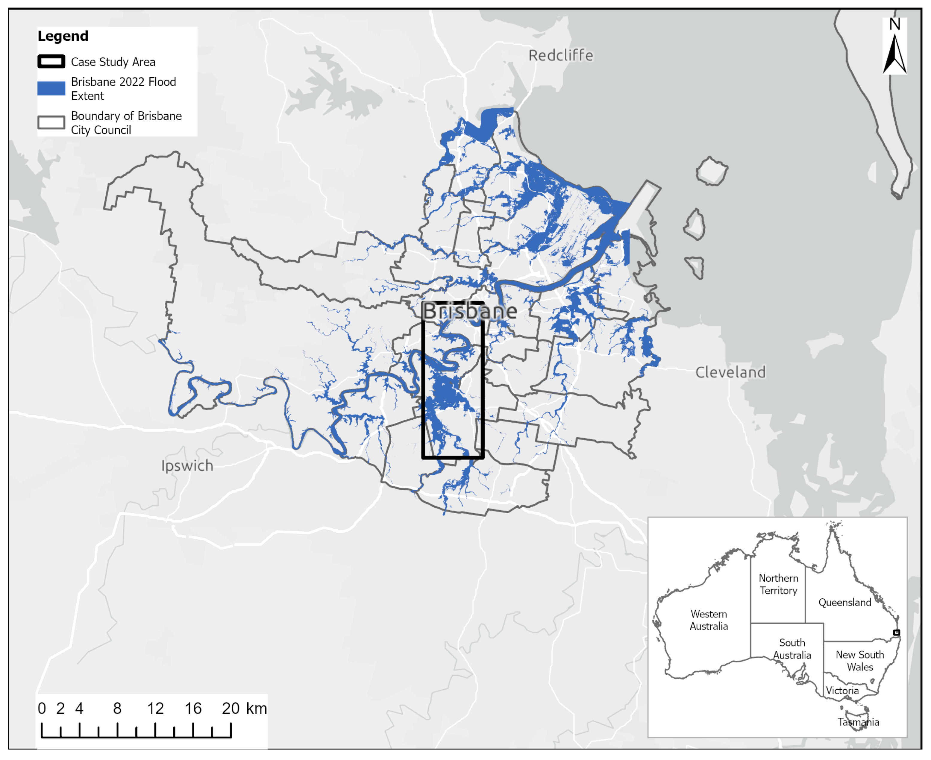
Figure 1.
The study area scope map about the February 2022 Brisbane flood using a dataset created by the Brisbane City Council. The entire flood extent was larger, containing other areas in Queensland and New South Wales. The case study is small compared to all of Australia.
Figure 1.
The study area scope map about the February 2022 Brisbane flood using a dataset created by the Brisbane City Council. The entire flood extent was larger, containing other areas in Queensland and New South Wales. The case study is small compared to all of Australia.
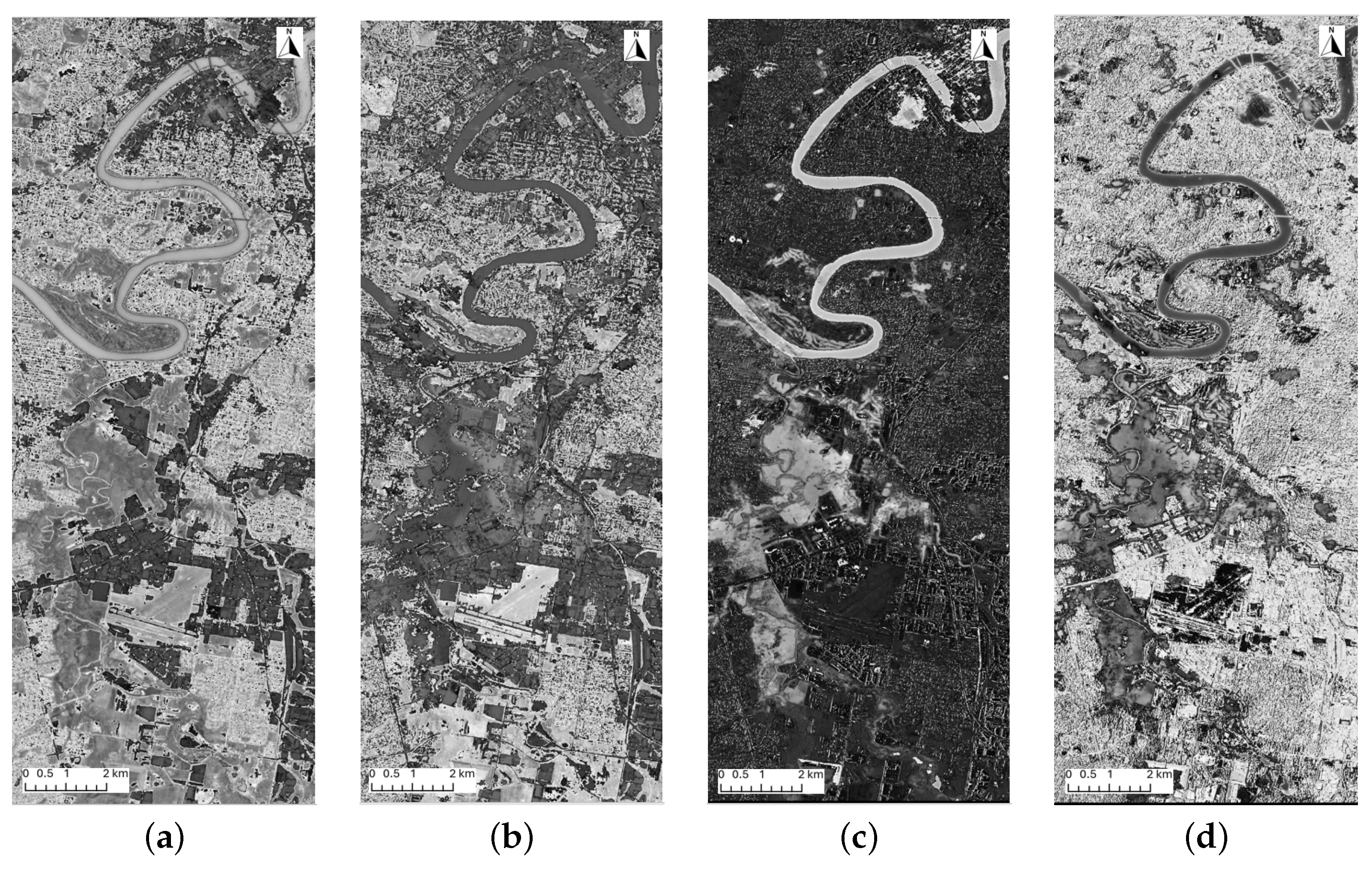
Figure 2.
(a) Pre-flooding PlanetScope image with natural colour, 9 February 2022. The case study contained an area from Brisbane’s CBD, through to the St. Lucia campus of the University of Queensland, to the flood plain of Oxley Creek in the south and Archerfield Airport; (b) pre-flooding PlanetScope image with false colour (NRG), 9 February 2022; (c) peak-flooding PlanetScope image with natural colour, 28 February 2022; (d) peak-flooding PlanetScope image with false colour (NRG), 28 February 2022.
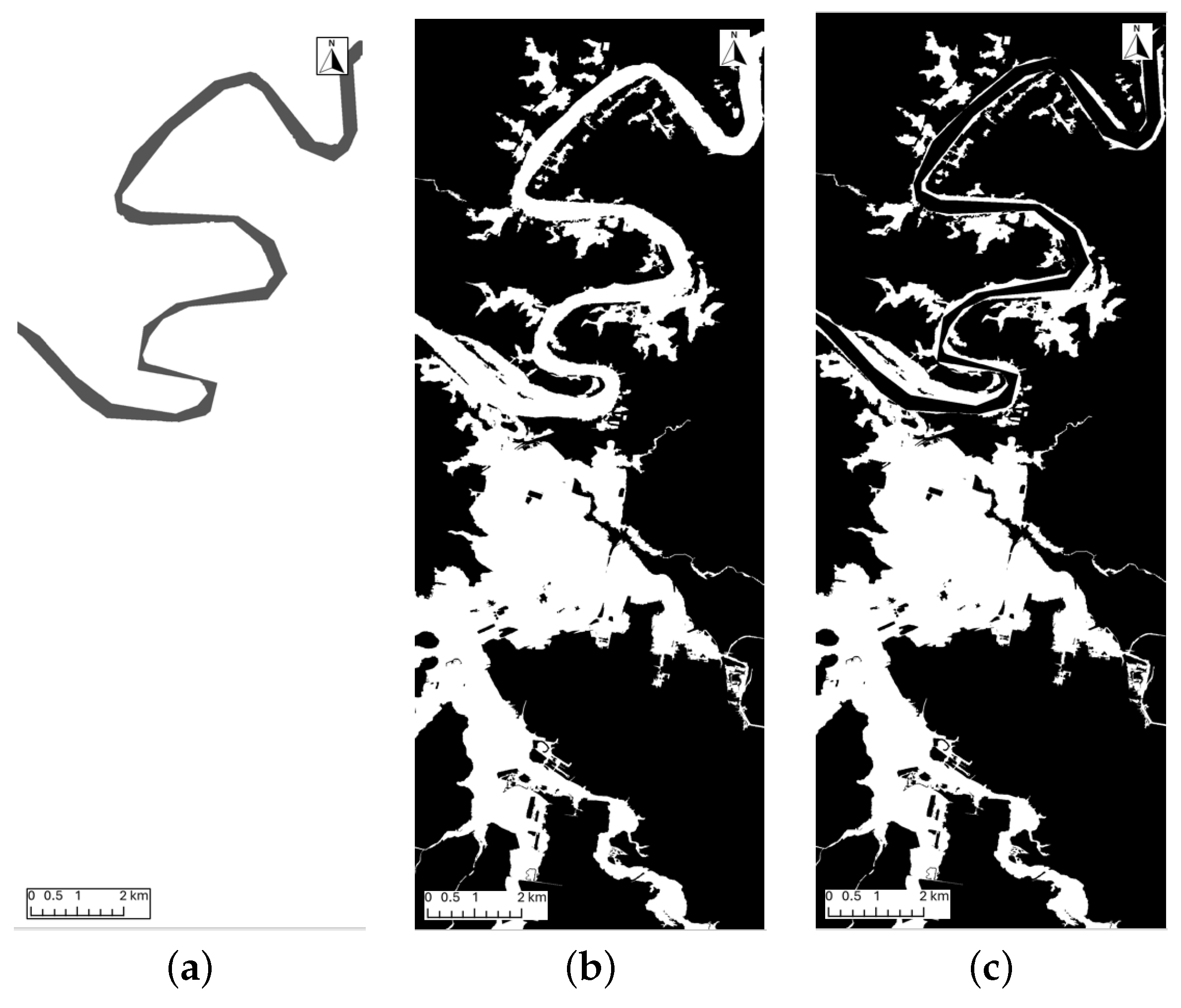
Figure 3.
(a) River-only image acquired from World Water Bodies, the black area represents the Brisbane River, whereas the white area represents others; (b) flood-only image acquired from BCC, where the white area represents flooding areas and the black area represents non-flooding areas; (c) labelled dataset image with the conjunction of (a,b) images with white areas set to flooded areas and the black area set as non-flooding area. Image (c) effectively removes the river from calculations.
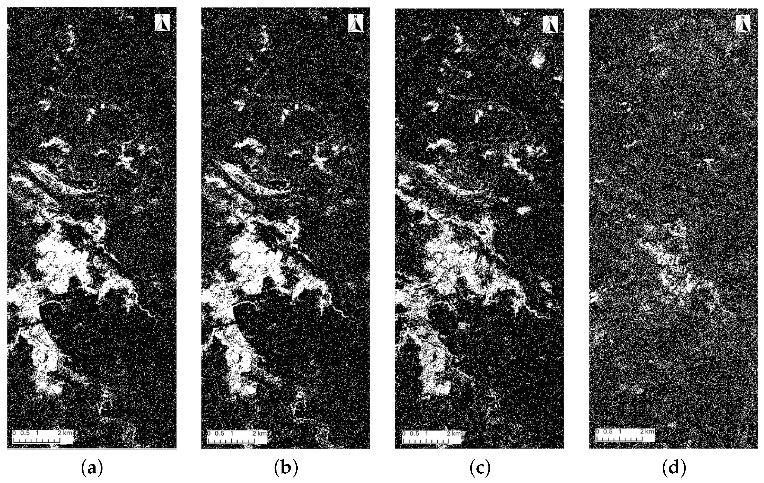
Figure 4.
Four images created using different spectral indices. (a) pre-NDWI image generated from pre-flooding PlanetScope image green and NIR bands; (b) peak-NDWI image generated from PlanetScope peak-flooding image green and NIR bands; (c) dNDWI image generated from peak-NDWI image subtracted pre-NDWI image; (d) NDII image generated from PlanetScope pre-flooding and peak-flooding images NIR band.
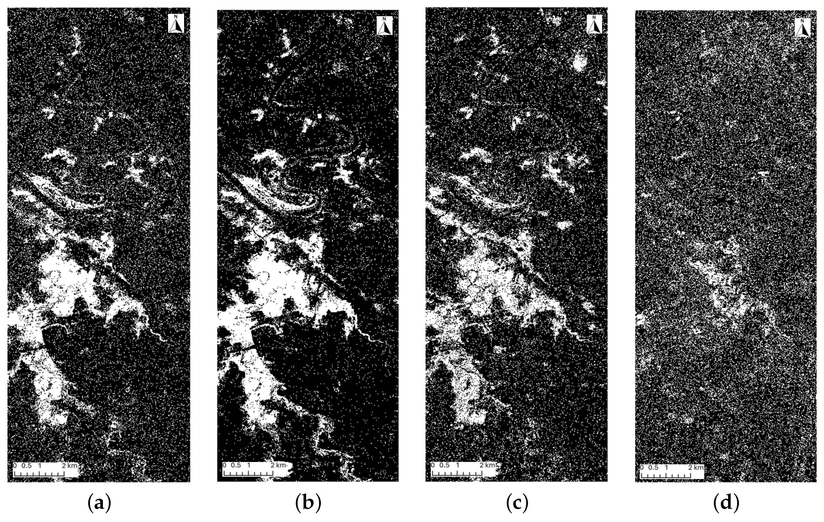
Figure 5.
Four DT-predicted flood maps using the four spectral indices. In each image, the white area represents flooding areas, whereas the black area represents non-flooding areas. (a) dNDWI-predicted flood map; (b) CNDWI-predicted flood map; (c) NDII-predicted flood map; (d) peak-NDWI-predicted flood map.
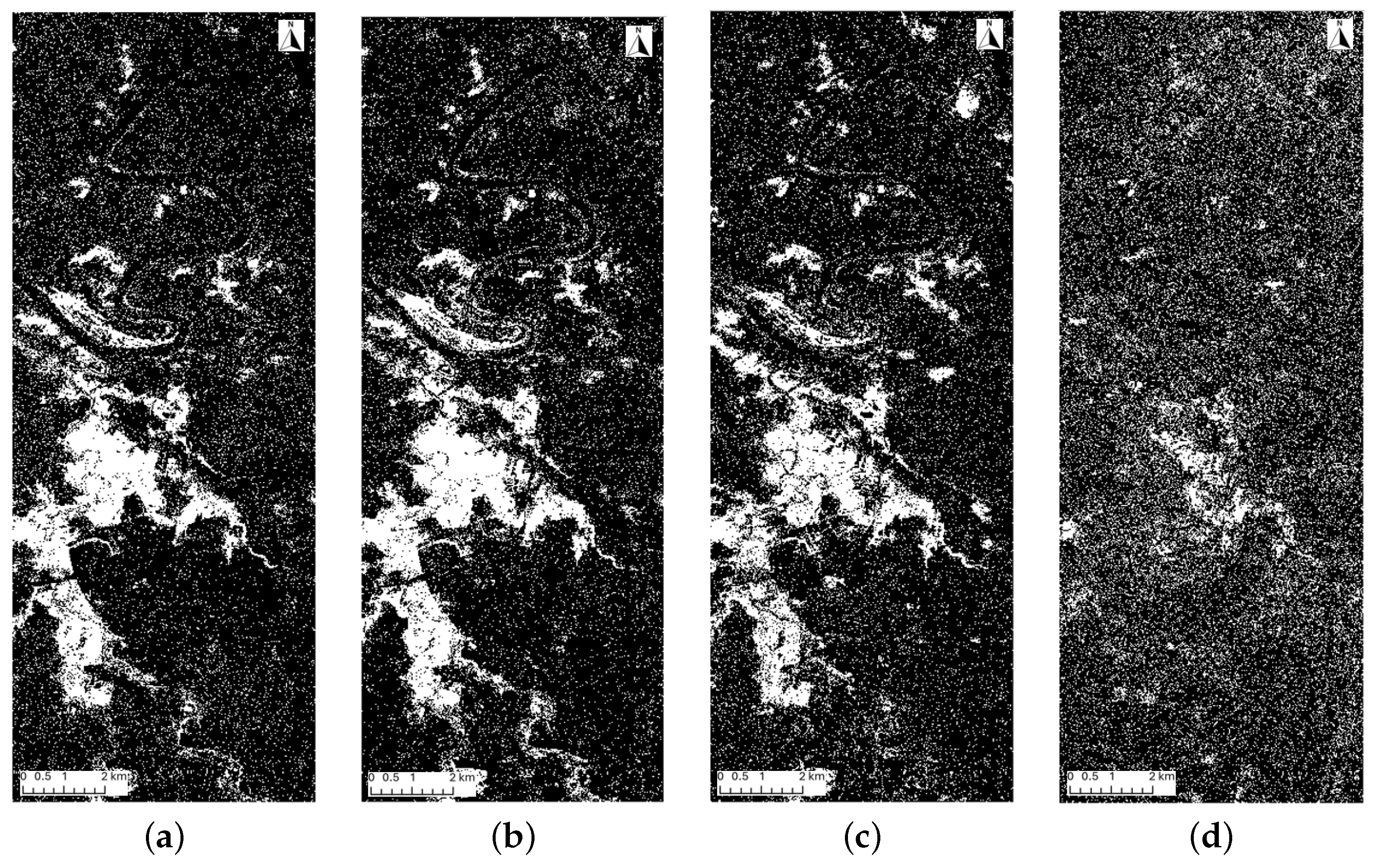
Figure 6.
Four RF-predicted flood maps using the four spectral indices. In each image, the white area represents flooding areas, whereas the black area represents non-flooding areas. (a) dNDWI-predicted flood map; (b) CNDWI-predicted flood map; (c) NDII-predicted flood map; (d) peak-NDWI-predicted flood map.
Figure 7.
Four NB-predicted flood maps using the four spectral indices. In each image, the white area represents flooding areas, whereas the black area represents non-flooding areas. (a) dNDWI-predicted flood map; (b) CNDWI-predicted flood map; (c) NDII-predicted flood map; (d) peak-NDWI-predicted flood map.
Figure 8.
Four KNN-predicted flood maps using the four spectral indices. In each image, the white area represents flooding areas, whereas the black area represents non-flooding areas. (a) dNDWI-predicted flood map; (b) CNDWI-predicted flood map; (c) NDII-predicted flood map; (d) peak-NDWI-predicted flood map.
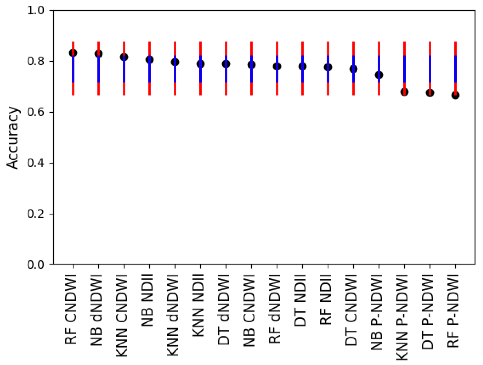
Figure 9.
The accuracy of the 16 experiments. The mean value was 0.769. The first standard deviation was 0.053 and the second standard deviation was 0.105. The standard error was 0.013. The two upper thresholds were 0.821 and 0.874. The two lower thresholds were 0.716 and 0.664. The lines for the two lower thresholds are blue whereas the lines for the two higher thresholds are red. RF CNDWI and NB dNDWI were above the first upper threshold. KNN, DT, and RF peak-NDWI were below the first lower threshold.
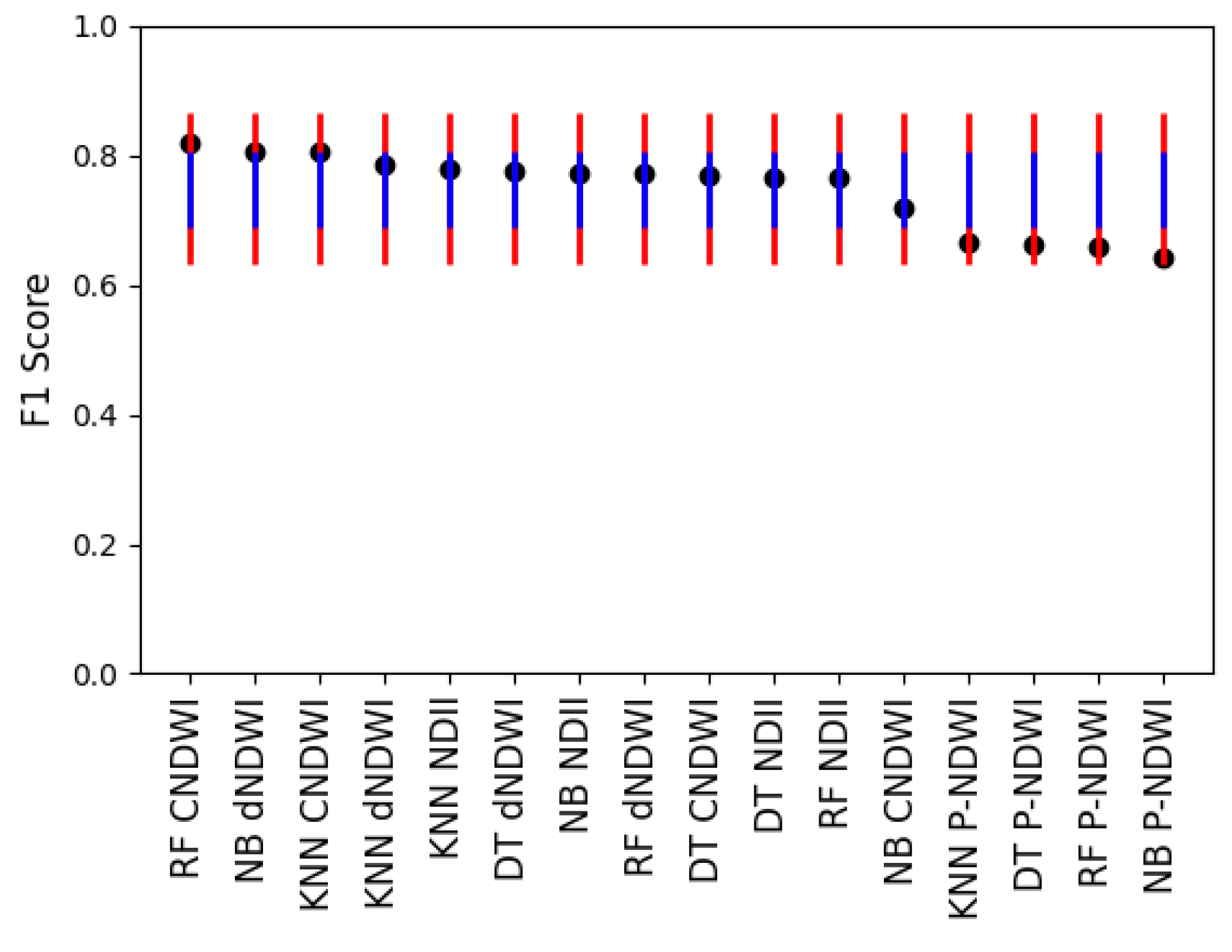
Figure 10.
The F1 Score of the 16 experiments. The mean value was 0.747. The first standard deviation was 0.058 and the second standard deviation was 0.117. The standard error was 0.015. The two upper thresholds were 0.806 and 0.864. The two lower thresholds were 0.689 and 0.630. The lines for the two lower thresholds are blue, whereas the lines for the two higher thresholds are red. RF CNDWI and NB dNDWI were above the first upper threshold. All the peak-NDWI algorithms were below the first lower threshold.
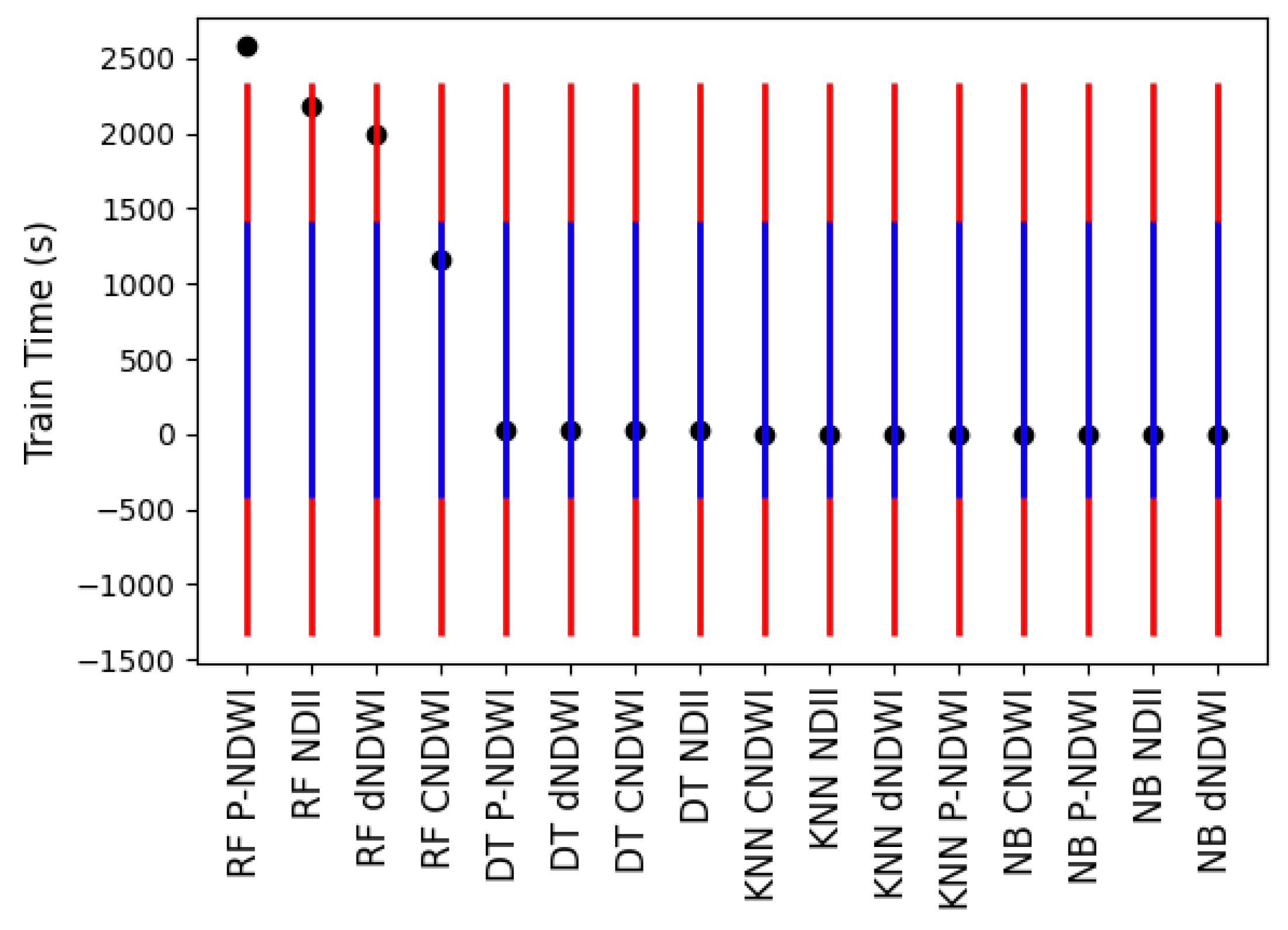
Figure 11.
The training time of the 16 experiments. The mean value was 502.099. The first standard deviation was 919.044 and the second standard deviation was 1838.089. The standard error was 229.761. The two upper thresholds were 1421.144 and 2340.188. The two lower thresholds were below 0. The lines for the two lower thresholds are blue whereas the lines for the two higher thresholds are red. RF peak-NDWI was above the second upper threshold. RF NDII and RF dNDWI were above the first upper threshold.
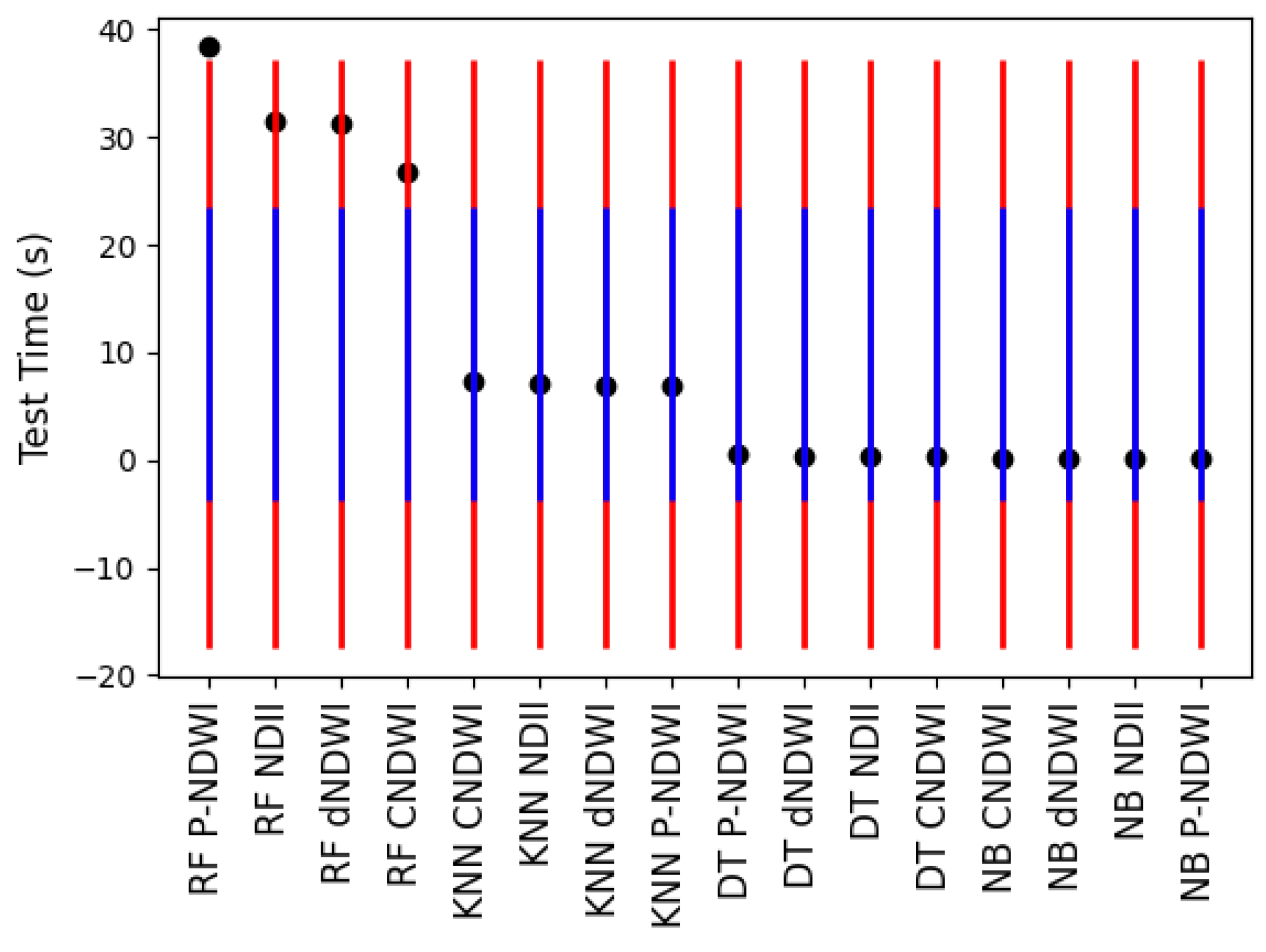
Figure 12.
The testing time of the 16 experiments. The mean value was 9.917. The first standard deviation was 13.664 and the second standard deviation was 27.329. The standard error was 3.416. The two upper thresholds were 23.581 and 37.246. Both two lower thresholds were below 0. The lines for the two lower thresholds are blue whereas the lines for the two higher thresholds are red. RF peak-NDWI was above the second upper thresholds. The rest of the RF indices were above the first threshold.
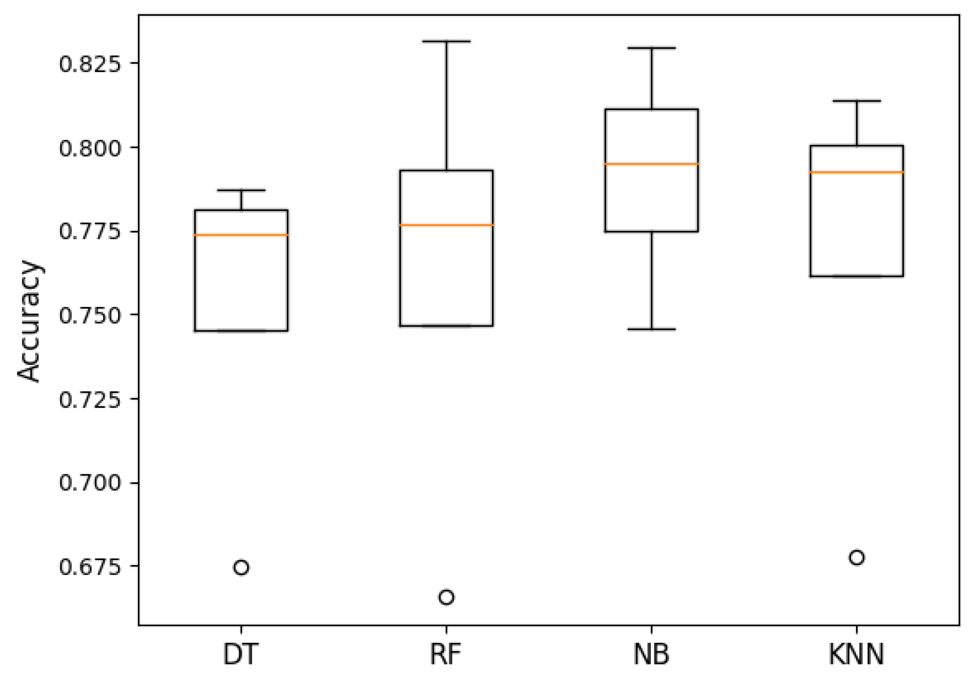
Figure 13.
Accuracy of ANOVA machine learning algorithms. The p-value was 0.796, meaning that there was no significant difference between the groups. The orange line represented the median accuracy of each algorithm. The circle represented outliers.
Figure 13.
Accuracy of ANOVA machine learning algorithms. The p-value was 0.796, meaning that there was no significant difference between the groups. The orange line represented the median accuracy of each algorithm. The circle represented outliers.
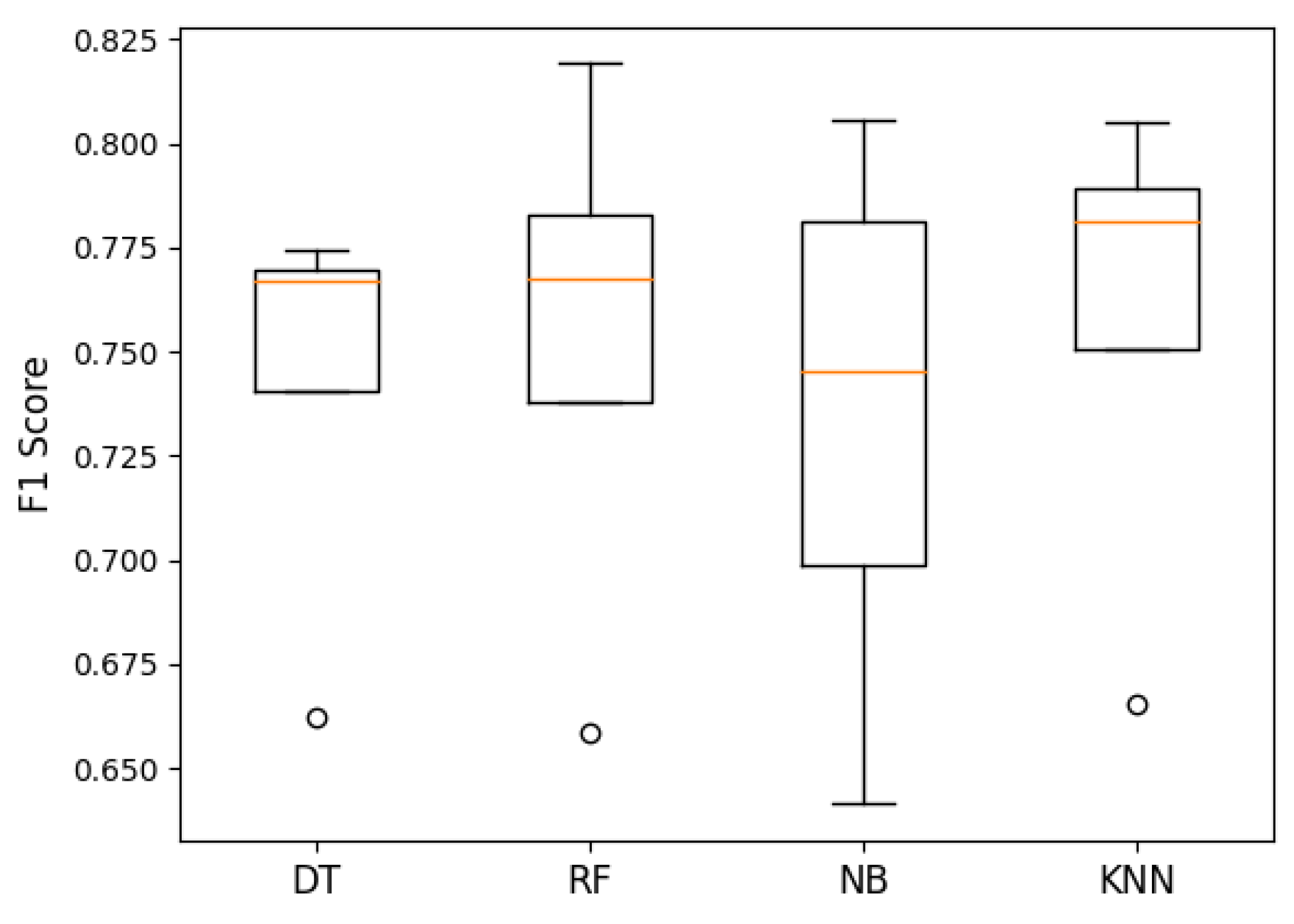
Figure 14.
F1 score of ANOVA machine learning algorithms. The p-value was 0.953, meaning that there was no significant difference between the groups. The orange line represented the median accuracy of each algorithm. The circle represented outliers.
Figure 14.
F1 score of ANOVA machine learning algorithms. The p-value was 0.953, meaning that there was no significant difference between the groups. The orange line represented the median accuracy of each algorithm. The circle represented outliers.
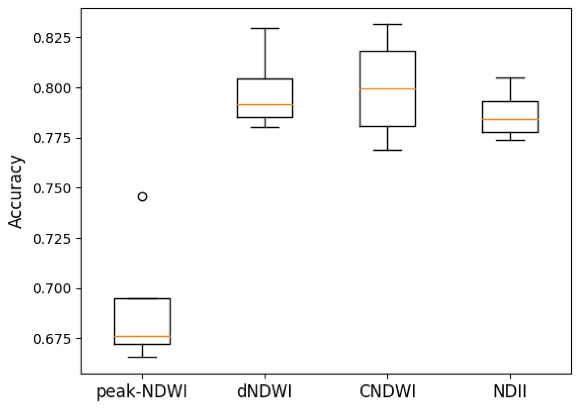
Figure 15.
Accuracy of ANOVA indices. The p-value was 2.023 , meaning that there was a significant difference between the groups. In this case, it was the peak-NDWI compared to the other indices. The orange line represented the median accuracy of each algorithm. The circle represented outliers.
Figure 15.
Accuracy of ANOVA indices. The p-value was 2.023 , meaning that there was a significant difference between the groups. In this case, it was the peak-NDWI compared to the other indices. The orange line represented the median accuracy of each algorithm. The circle represented outliers.
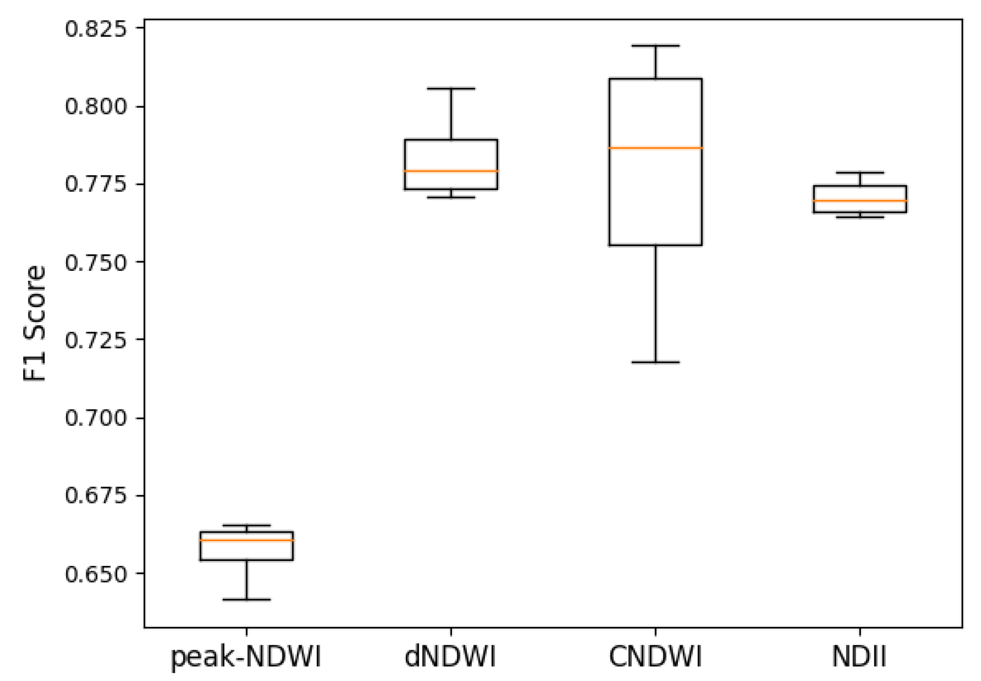
Figure 16.
F1 score of ANOVA indices. The p-value was 2.482 , meaning that there was a significant difference between the groups. In this case, it was the peak-NDWI and the other indices. The orange line represented the median accuracy of each algorithm. The circle represented outliers.
Figure 16.
F1 score of ANOVA indices. The p-value was 2.482 , meaning that there was a significant difference between the groups. In this case, it was the peak-NDWI and the other indices. The orange line represented the median accuracy of each algorithm. The circle represented outliers.
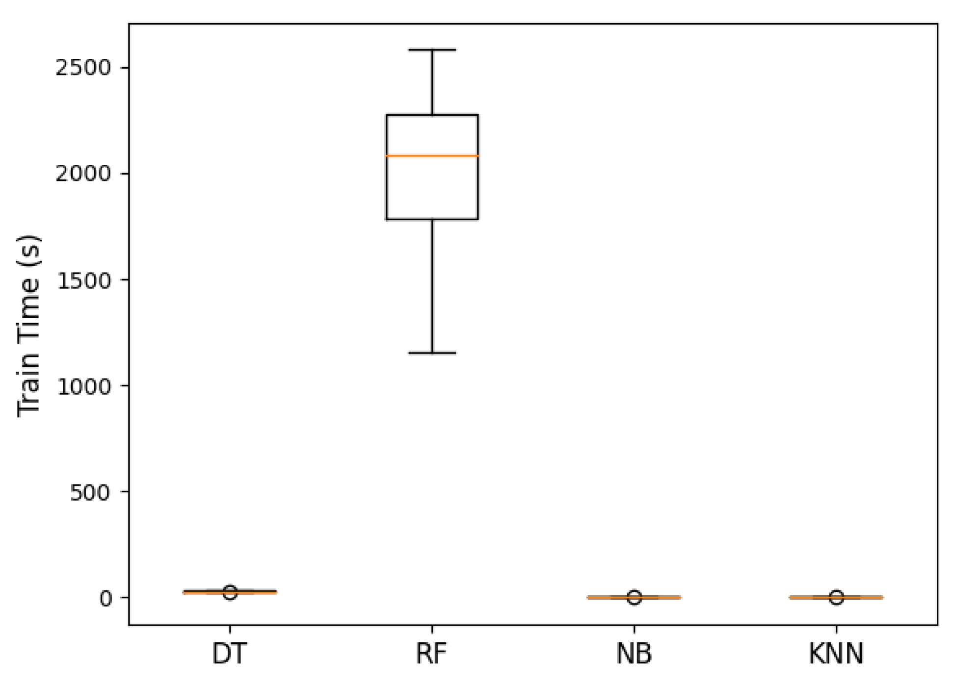
Figure 17.
ANOVA machine learning training time (s). The p-value was 1.055 , meaning that there was a significant difference between the groups. In this case, it was the Random Forest algorithm compared to the other machine learning algorithms. The orange line represented the median accuracy of each algorithm. The circle represented outliers.
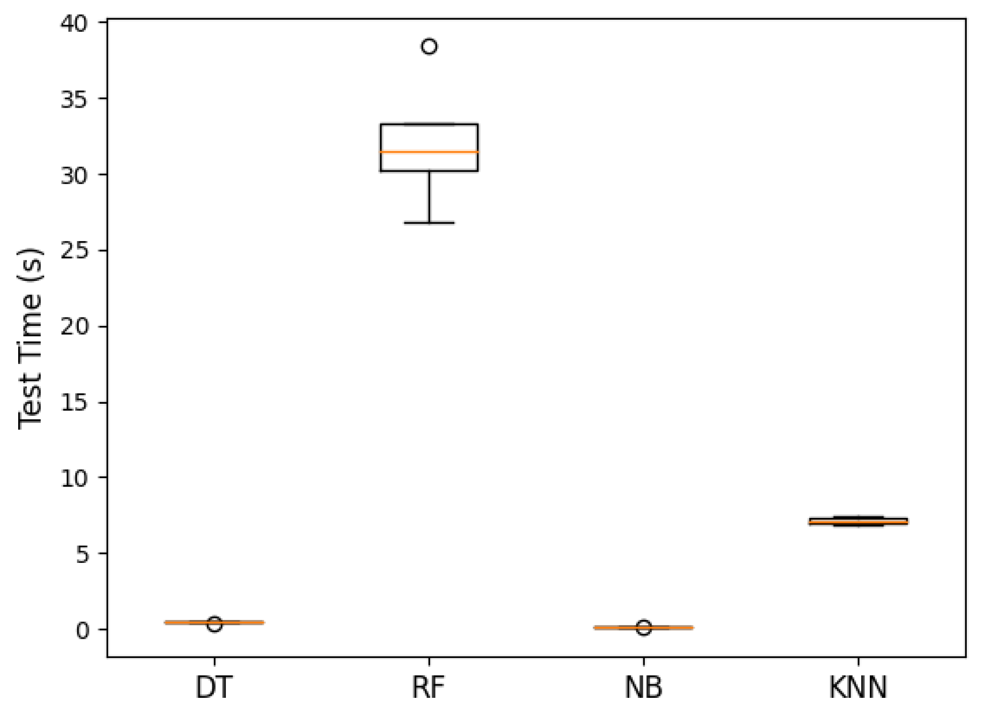
Figure 18.
ANOVA machine learning testing time (s). The p-value was 6.273 , meaning that there was a significant difference between the groups. In this case, it was the Random Forest and K-Nearest Neighbours algorithms compared to the other machine learning algorithms. The orange line represented the median accuracy of each algorithm. The circle represented outliers.
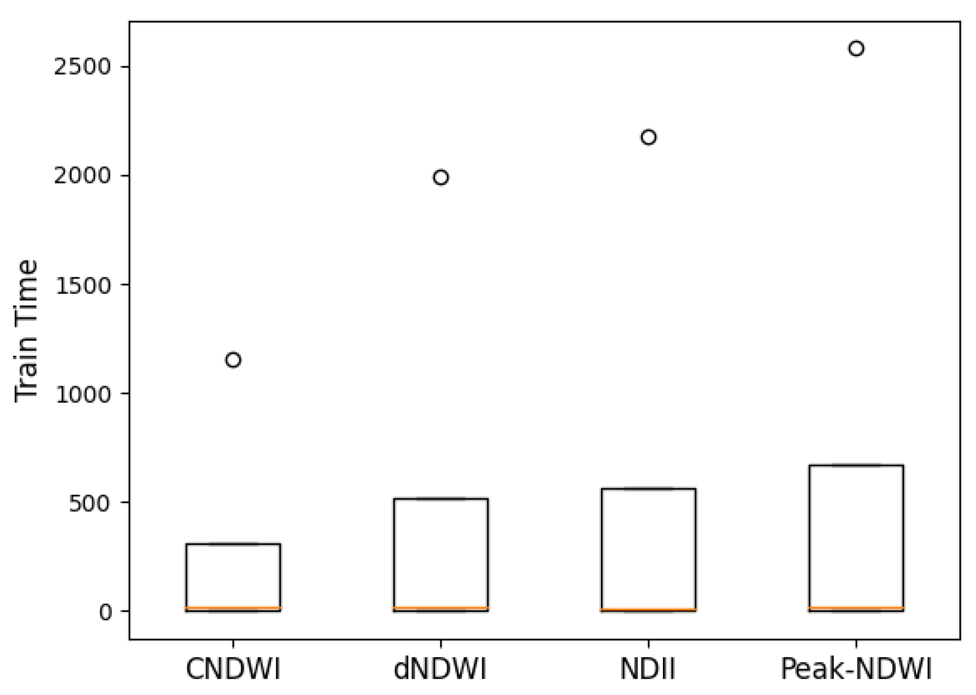
Figure 19.
ANOVA indices training time (s). The p-value was 0.995, meaning that there was not a significant difference between the groups. The orange line represented the median accuracy of each algorithm. The circle represented outliers.
Figure 19.
ANOVA indices training time (s). The p-value was 0.995, meaning that there was not a significant difference between the groups. The orange line represented the median accuracy of each algorithm. The circle represented outliers.
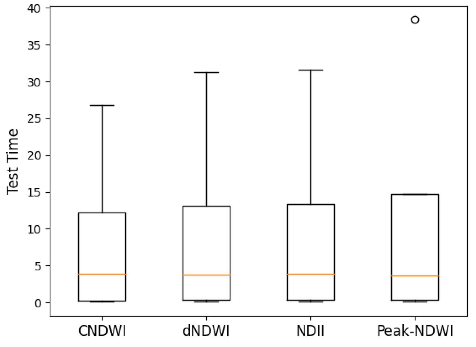
Figure 20.
ANOVA indices testing time (s). The p-value was 0.966, meaning that there was not a significant difference between the groups. The orange line represented the median accuracy of each algorithm. The circle represented outliers.
Figure 20.
ANOVA indices testing time (s). The p-value was 0.966, meaning that there was not a significant difference between the groups. The orange line represented the median accuracy of each algorithm. The circle represented outliers.
Table 1.
Details of spectral bands (blue, green, red, NIR, and SWIR) with band type and wavelength ranges.
Table 1.
Details of spectral bands (blue, green, red, NIR, and SWIR) with band type and wavelength ranges.
| Band | Type | Wavelengths Range (nm) |
|---|
| Blue | Visible | 455–515 |
| Green | Visible | 500–590 |
| Red | Visible | 590–670 |
| Near infrared (NIR) | Invisible | 780–860 |
Table 2.
Spectral indices formula.
Table 2.
Spectral indices formula.
| Spectral Index | Formula |
|---|
| Normalised Difference Water Index | |
| Differential Normalised Difference Water Index (dNDWI) | |
| Normalised Difference Inundation Index (NDII) | |
Table 3.
Machine learning algorithms big O complexity in training and test time.
Table 3.
Machine learning algorithms big O complexity in training and test time.
| Machine Learning Algorithms | Characteristics | Construction Model | Classification Category | Training Complexity | Test Complexity |
|---|
| Decision Tree | State Trees | Single | Non-linear | | |
| Random Forest | State Trees | Ensemble | Non-linear | | |
| Naive Bayes | Conditional Probability Trees | Single | Linear | | |
| K-Nearest Neighbour | Proximity Based | Single | Non-linear | O(1) | |
Table 4.
Information about the Labelled Dataset, BCC generated it from both river and creek flooding in a shape file.
Table 4.
Information about the Labelled Dataset, BCC generated it from both river and creek flooding in a shape file.
| Description | Value |
|---|
| Spatial Pixel Size (m) | 4.55 × 5.11 |
| Image Size (km2) | 88.80 |
| Width (pixels) | 1184 |
| Length (pixels) | 3081 |
| Area (pixels) | 3,647,904 |
| Flooded Area (pixels) | 938,033 |
| Non-Flooded Area (pixels) | 2,709,871 |
| Percent Flooded (percent) | 25.71 |
| Percent Non-Flooded (percent) | 74.29 |
Table 5.
Accuracy table for combining the four ML algorithms and the four types of indices.
Table 5.
Accuracy table for combining the four ML algorithms and the four types of indices.
| Algorithm | Index | Accuracy |
|---|
| RF | CNDWI | 0.831 * |
| NB | dNDWI | 0.830 * |
| KNN | CNDWI | 0.814 |
| NB | NDII | 0.805 |
| KNN | dNDWI | 0.796 |
| KNN | NDII | 0.789 |
| DT | dNDWI | 0.787 |
| NB | CNDWI | 0.785 |
| RF | dNDWI | 0.780 |
| DT | NDII | 0.779 |
| RF | NDII | 0.774 |
| DT | CNDWI | 0.769 |
| NB | peak-NDWI | 0.746 |
| KNN | peak-NDWI | 0.678 - |
| DT | peak-NDWI | 0.675 - |
| RF | peak-NDWI | 0.666 - |
Table 6.
F1 score table for combining the four ML algorithms and the four types of indices.
Table 6.
F1 score table for combining the four ML algorithms and the four types of indices.
| Algorithm | Index | F1 Score |
|---|
| RF | CNDWI | 0.819 * |
| NB | dNDWI | 0.806 * |
| KNN | CNDWI | 0.805 |
| KNN | dNDWI | 0.784 |
| KNN | NDII | 0.779 |
| DT | dNDWI | 0.774 |
| NB | NDII | 0.773 |
| RF | dNDWI | 0.770 |
| DT | CNDWI | 0.768 |
| DT | NDII | 0.766 |
| RF | NDII | 0.765 |
| NB | CNDWI | 0.718 |
| KNN | peak-NDWI | 0.666 - |
| DT | peak-NDWI | 0.662 - |
| RF | peak-NDWI | 0.659 - |
| NB | peak-NDWI | 0.641 - |
Table 7.
Train time for combining the four ML algorithms and the four types of indices.
Table 7.
Train time for combining the four ML algorithms and the four types of indices.
| Algorithm | Index | Train Time (s) |
|---|
| RF | peak-NDWI | 2580.282 ** |
| RF | NDII | 2178.655 * |
| RF | dNDWI | 1988.481 * |
| RF | CNDWI | 1158.142 |
| DT | peak-NDWI | 31.429 |
| DT | dNDWI | 30.088 |
| DT | CNDWI | 29.989 |
| DT | NDII | 27.374 |
| KNN | CNDWI | 2.936 |
| KNN | NDII | 1.903 |
| KNN | dNDWI | 1.794 |
| KNN | peak-NDWI | 1.759 |
| NB | CNDWI | 0.394 |
| NB | peak-NDWI | 0.125 |
| NB | NDII | 0.121 |
| NB | dNDWI | 0.118 |
Table 8.
Test time for combining the four ML algorithms and the four types of indices.
Table 8.
Test time for combining the four ML algorithms and the four types of indices.
| Algorithm | Index | Test Time(s) |
|---|
| RF | peak-NDWI | 38.397 ** |
| RF | NDII | 31.581 * |
| RF | dNDWI | 31.308 * |
| RF | CNDWI | 26.818 * |
| KNN | CNDWI | 7.383 |
| KNN | NDII | 7.223 |
| KNN | dNDWI | 7.016 |
| KNN | peak-NDWI | 6.819 |
| DT | peak-NDWI | 0.481 |
| DT | dNDWI | 0.463 |
| DT | NDII | 0.459 |
| DT | CNDWI | 0.342 |
| NB | CNDWI | 0.112 |
| NB | dNDWI | 0.094 |
| NB | NDII | 0.090 |
| NB | peak-NDWI | 0.087 |
Table 9.
The ANOVA p-value across ML algorithms, indices, and time with different measures: accuracy, F1 score, training time, and test time. Underlined values mean that the p-values were less than 0.05.
Table 9.
The ANOVA p-value across ML algorithms, indices, and time with different measures: accuracy, F1 score, training time, and test time. Underlined values mean that the p-values were less than 0.05.
| Experiment Type | p-Value |
|---|
| ML Accuracy | 0.796 |
| ML F1 Score | 0.953 |
| Indices Accuracy | 2.023 |
| Indices F1 Score | 2.482 |
| ML Training Time | 1.055 |
| ML Test Time | 6.273 |
| Indices Training Time | 0.995 |
| Indices Test Time | 0.966 |
Table 10.
The HSD results of the machine learning algorithms’ accuracy. The p-value was 0.796, meaning that there was no significant difference between the groups. For clarity, the comparisons between the same group are greyed.
Table 10.
The HSD results of the machine learning algorithms’ accuracy. The p-value was 0.796, meaning that there was no significant difference between the groups. For clarity, the comparisons between the same group are greyed.
| ML | DT | RF | NB | KNN |
|---|
| DT | | 0.9935 | 0.7646 | 0.9729 |
| RF | 0.9935 | | 0.8884 | 0.9983 |
| NB | 0.7646 | 0.8884 | | 0.9444 |
| KNN | 0.9729 | 0.9983 | 0.9444 | |
Table 11.
The HSD results of the machine learning algorithms’ F1 score. The p-value was 0.953, meaning that there was no significant difference between the groups. For clarity, the comparisons between the same group are greyed.
Table 11.
The HSD results of the machine learning algorithms’ F1 score. The p-value was 0.953, meaning that there was no significant difference between the groups. For clarity, the comparisons between the same group are greyed.
| ML | DT | RF | NB | KNN |
|---|
| DT | | 0.9954 | 0.9978 | 0.9854 |
| RF | 0.9954 | | 0.9756 | 0.9995 |
| NB | 0.9978 | 0.9756 | | 0.9519 |
| KNN | 0.9854 | 0.9995 | 0.9519 | |
Table 12.
The HSD results of the indices’ accuracy. The p-value was 2.023 , meaning that there was a significant difference between the groups. In this case, it was the peak-NDWI compared to the other indices. For clarity, the comparisons between the same group are greyed.
Table 12.
The HSD results of the indices’ accuracy. The p-value was 2.023 , meaning that there was a significant difference between the groups. In this case, it was the peak-NDWI compared to the other indices. For clarity, the comparisons between the same group are greyed.
| Index | Peak-NDWI | dNDWI | CNDWI | NDII |
|---|
| Peak-NDWI | | 0.0005 | 0.0004 | 0.0013 |
| dNDWI | 0.0005 | | 0.9998 | 0.9286 |
| CNDWI | 0.0004 | 0.9998 | | 0.9017 |
| NDII | 0.0013 | 0.9286 | 0.9017 | |
Table 13.
The HSD results of the indices’ F1 score. The p-value was 2.482 , meaning that there was a significant difference between the groups. In this case, it was the peak-NDWI compared to the other indices. For clarity, the comparisons between the same group are greyed.
Table 13.
The HSD results of the indices’ F1 score. The p-value was 2.482 , meaning that there was a significant difference between the groups. In this case, it was the peak-NDWI compared to the other indices. For clarity, the comparisons between the same group are greyed.
| Index | Peak-NDWI | dNDWI | CNDWI | NDII |
|---|
| Peak-NDWI | | 0.0001 | 0.0001 | 0.0002 |
| dNDWI | 0.0001 | | 0.9849 | 0.8830 |
| CNDWI | 0.0001 | 0.9849 | | 0.9800 |
| NDII | 0.0002 | 0.8830 | 0.9800 | |
Table 14.
The HSD results of the machine learning algorithms’ training time. The p-value was 1.055 , meaning that there was a significant difference between the groups. In this case, it was the Random Forest algorithm compared to the other machine learning algorithms. For clarity, the comparisons between the same group are greyed.
| ML | DT | RF | NB | KNN |
|---|
| DT | | <0.0001 | 0.9990 | 0.9992 |
| RF | <0.0001 | | <0.0001 | <0.0001 |
| NB | 0.9990 | <0.0001 | | 1.0000 |
| KNN | 0.9992 | <0.0001 | 1.0000 | |
Table 15.
The HSD results of the machine learning algorithms’ testing time. The p-value was 6.273 , meaning that there was a significant difference between the groups. In this case, it was the Random Forest and K-Nearest Neighbours algorithms compared to the other machine learning algorithms. For clarity, the comparisons between the same group are greyed.
| ML | DT | RF | NB | KNN |
|---|
| DT | | <0.0001 | 0.9969 | 0.0091 |
| RF | <0.0001 | | <0.0001 | <0.0001 |
| NB | 0.9969 | <0.0001 | | 0.0064 |
| KNN | 0.0091 | <0.0001 | 0.0064 | |
Table 16.
The HSD results of the indices’ training time. The p-value was 0.995, meaning that there was not a significant difference between the groups. For clarity, the comparisons between the same group are greyed.
Table 16.
The HSD results of the indices’ training time. The p-value was 0.995, meaning that there was not a significant difference between the groups. For clarity, the comparisons between the same group are greyed.
| Index | Peak-NDWI | dNDWI | CNDWI | NDII |
|---|
| Peak-NDWI | | 0.9985 | 0.9936 | 0.9987 |
| dNDWI | 0.9985 | | 0.9996 | 1.0000 |
| CNDWI | 0.9936 | 0.9996 | | 0.9995 |
| NDII | 0.9987 | 1.0000 | 0.9995 | |
Table 17.
The HSD results of the indices’ testing time. The p-value was 0.966, meaning that there was not a significant difference between the groups. For clarity, the comparisons between the same group are greyed.
Table 17.
The HSD results of the indices’ testing time. The p-value was 0.966, meaning that there was not a significant difference between the groups. For clarity, the comparisons between the same group are greyed.
| Index | Peak-NDWI | dNDWI | CNDWI | NDII |
|---|
| Peak-NDWI | | 0.9967 | 0.9588 | 0.9989 |
| dNDWI | 0.9967 | | 0.9912 | 0.9999 |
| CNDWI | 0.9588 | 0.9912 | | 0.9841 |
| NDII | 0.9989 | 0.9999 | 0.9841 | |


