Article

Examining the Long-Run and Short-Run Relationship between Water Demand and Socio-Economic Explanatory Variables: Evidence from Amman

1
Department of Civil Engineering, Yarmouk University, Irbid 21163, Jordan
2
Department of Civil Engineering, Jadara University, Irbid 21110, Jordan
*
Author to whom correspondence should be addressed.
Sustainability 2024, 16(6), 2315; https://doi.org/10.3390/su16062315
Submission received: 6 January 2024 / Revised: 26 February 2024 / Accepted: 1 March 2024 / Published: 11 March 2024

Abstract

:
This study investigates the key factors that influence household water usage in Amman, Jordan, with the aim of improving water management practices in a region facing significant scarcity. The research focuses on factors such as temperature, water pricing, system input, and family size. The Vector Error Correction Model with Exogenous Variables (VECMX) is applied to data from 1980 to 2015 to provide insights into consumption patterns, both in the short-term and long-term. The results show that family size and marginal costs significantly impact long-term water demand, while system input and family size influence short-term water demand. The study also finds that water pricing has a limited impact on consumer behavior, indicating inelasticity. Temperature and income, however, did not emerge as significant determinants. These findings highlight the need for water management policies in arid areas like Amman to prioritize factors other than price, such as household size and water infrastructure, to establish more effective strategies for conserving water.

1. Introduction

Jordan’s capital city, Amman, is currently grappling with water scarcity due to its hot and arid climate during summers and milder winters [1,2]. However, despite the challenges, Amman continues to be the economic, social, and cultural center of Jordan; it has an impressive population exceeding 4.5 million spread across nine districts and an area of 7579 square kilometers [3].
Historically and currently, Amman has been experiencing severe water scarcity due to a combination of factors. The city’s rapid economic expansion, rapidly growing population, and influx of refugees have all contributed to a significant increase in water demand. In addition, the impact of climate change has made water availability increasingly uncertain, while urbanization has placed additional pressure on the already limited water supply [4,5]. As a result, the current state of the city’s water supply is a growing concern, as the water demand is surpassing the available resources [6,7,8]. This issue is particularly pronounced during the summer months, leaving the city exposed to the risk of droughts.
To optimize the utilization of freshwater resources, it is imperative for Amman’s water utility not only to invest in new resources but also to implement effective demand management policies. By doing so, the utility can minimize potential welfare losses arising from demand-supply deficits. Therefore, an accurate water demand forecast is critical to this process. A multivariate approach to analyzing and forecasting water demand can offer valuable insights and guidance for water management. Within the context of this framework, it is possible to assess the effectiveness of socio-economic factors in managing demand.
Many studies have attempted to predict the water demand in Amman by utilizing a multivariate modeling approach. However, most of these studies have focused on short-term forecasting using cross-section panel data, and there needs to be more research on long-term forecasting utilizing time-series data. For instance, Al-Najjar et al.’s (2011) [9] research used two-stage least squares (2SLS) to analyze quarterly aggregate panel data for Amman. Salman and Al-Karablieh (2006) [10] used the Ordinary Least Square method to study quarterly aggregate panel data for Jordan. Tabieh et al. (2012) [11] analyzed cross-section data from the Zarka Basin using two stages of least squares (2SLS). Telfah et al. (2021) [8] utilized an autoregressive distributed lag (ARDL) model to analyze time-series data from Amman.
In order to evaluate the potential of socio-economic factors as a demand management tool in Amman, it is critical to maintain a comprehensive understanding of the elasticity of water demand relative to each of these factors. Therefore, the purpose of the study is to formulate and estimate a dynamic model of water consumption in Amman using a Vector Error Correction Model with Exogenous Variables (VECMX). It aims to estimate variables that affect short-term and long-term water demand using aggregated annual data from 1980 to 2015, concentrating on significant determinants such as income, per-subscriber water usage, water supply quantity, marginal price, temperature, and family size. This approach offers a thorough understanding of water demand dynamics in Amman, which could serve as a worldwide blueprint for water utility companies, policymakers, and urban planners facing similar challenges. The model is a critical tool for strategic planning to ensure efficient and sustainable water resource management.
This study pursues to make a significant academic contribution by utilizing a vector error correction model with exogenous variables (VECMX) to analyze water demand in Amman. It realizes the shortcomings of traditional vector autoregressive (VAR) models in dealing with stationary cointegrated variables at the first difference level. To overcome the above challenges, the study has implemented the Vector Error Correction Model with Exogenous Variables (VECMX).
Forecasting the water demand in Amman is challenging due to the constrained reliability of accessible data and the large number of variables that impact it [12]. Further research may involve including novel variables, such as developments in water conservation technologies. Moreover, extending the model’s application to other regions that face similar water scarcity issues and exploring alternative modeling techniques can be beneficial in extending our understanding and approach toward global water management challenges.
The paper is structured as follows: Section 1 introduces the study, Section 2 reviews existing literature, Section 3 describes our methodology, Section 4 presents the Results, and subsequent sections discuss the results, implications, and conclusions drawn from our findings.

2. Literature Review

Recent research on domestic water demand has used various models to understand its correlation with influencing factors [13,14]. The results of the models are used as a basis for developing policies and strategies. The models may be static, dynamic, short, medium, or long-term, considering different water sources. Water demand forecasting in the context of intermittent water supply in arid regions (as in this study) has been studied to identify primary factors influencing water demand. Examples are found in [11,15,16,17,18].
In the literature, various explanatory variables have been identified as determinants of water demand, including economic variables like water price, income, and water pricing structure. Climatic and weather factors, such as temperature, rainfall, drought, and demographic characteristics, like population size, household composition, and urban congestion, also play a role. Technological innovations and resource availability are significant determinants as well. Additionally, non-price controls like conservation campaigns, incentives, and legislation have been taken into account when measuring water demand [18,19,20,21].
Several techniques are employed to predict water consumption, which are designed to cater to particular requirements. Both qualitative and quantitative methodologies are implemented. Quantitative approaches analyze several types of data, including cross-sectional, time series, and panel data, applying advanced methods such as artificial neural networks [22,23,24,25,26], time series analysis [17,27,28,29,30] regression models [31,32], fuzzy models [33], the Kalman filter technique [34,35], the linear quadratic estimator [36], and hybrid models [26]. The selection of these methods relies on the features of the data and the specific needs for predicting, thereby enhancing the reliability and effectiveness of municipal water management.
This study utilizes the methodologies of co-integration (Engle and Granger, 1987) [30,37,38] and error correction to estimate the dynamics of determinants of municipal water use in Amman.
Water demand estimation literature has thoroughly examined pricing elasticity’s effectiveness in predicting revenue, conservation responses, and water conservation. Numerous surveys and meta-analyses have documented this literature (for instance, [12,39,40,41,42,43,44]). In contrast, most studies indicate inelastic household water demand estimates (<1) [12,44] and some cases provide elastic estimates (>1) [45]. Elastic demand indicates that even a slight price increase may substantially decrease water usage, reducing revenue but improving conservation. Due to inelastic demand, a slight price increase has minimal impact on the use of water, leading to more revenue but inadequate conservation.
Water price-elasticity estimations vary per study. Sabri (2014) [40] evaluated 100 studies and generated 638 price elasticity estimates, averaging −0.365 and medianing −0.291, ranging from −3.054 to −0. 002. Reynaud (2015) [39] estimated that the water price elasticity for 28 EU countries is between −0.5 and −0.1. According to existing literature, long-run price elasticities are typically higher (in absolute value) than short-run elasticities (for instance, [14,40,46,47,48]).
Recent research has unearthed a positive correlation between household water usage and income, probably due to more water-dependent facilities and comforts, including outdoor recreational places and domestic appliances [39]. Literature research suggests that income minimally affects water consumption, as income elasticity estimates typically fall below one; this can be related to budgetary constraints and consumer ignorance of water costs.
Different studies have found different income elasticity. According to Reynaud (2015) [39], Western European countries have low-income elasticities (0.00–0.25), while Eastern European countries have larger elasticities (>0.50). Sabri (2014) [40] analyzed 72 studies and obtained 332 income elasticity estimates, averaging 0.207 and medianing 0.159, ranging from −0.440 to 1.560. Dalhuisen (2003) [43] documented that the income elasticities had an average value of 0.43 and a median of 0.24.
Extensive scholarly literature underscores the significance of household sizes in determining residential water consumption. Examples are in Refs. [12,42,49]. As the number of people in a household increases, the total consumption also increases. However, the per capita consumption decreases due to economies of scale. Considering household size in water pricing is essential for achieving equity targets and managing demand [50,51]. A meta-analysis conducted by Sebri (2014) [40], which included 23 studies, reported that the mean and median household size elasticities were 0.355 and 0.322, respectively, with a range of 0.011 to 1.410. Another critical factor in determining residential consumption is the household size or the number of individuals living there [12,42,49].
The existing scholarly literature on the relationship between water supply and residential water consumption is deemed insufficient. This inadequacy is mirrored in the fact that in most developed countries, the water supply is able to meet the desired level of water demand. According to Telfah et al. (2021) [52], water supply positively and significantly impacts water consumption in countries experiencing water scarcity. Specifically, they estimate the elasticity of system input to be 0.47.
Multiple studies have analyzed the impact of temperature on water demand. These explorations revealed that the influence of temperature on water demand varies across regions and local climates, with inconsistent levels of temperature elasticity [21]. Cabral et al. (2016) [53] documented that temperature significantly influences water consumption. Hoffmann et al. (2006) [20] argue that a 10% growth in warm days leads to a 0.01% increase in water consumption. Romano et al. (2014) [54] encounter no influence of temperature on drinking water consumption for domestic use. Maidment and Miaou (1986) [55] remark no effect of daily maximum air temperature between 40 °F and 70 °F; beyond 70 °F, water demand increases with temperature. It is crucial to debate that temperature elasticity in water demand should be analyzed on a regional or local level, as it is clear that this concept cannot be applied universally [21].

3. Materials and Methods

The Vector Error Correction Model with Exogenous Variables (VECMX) was thoughtfully selected for analyzing water demand in Amman due to its unique ability to analyze both short-term and long-term dynamics between water demand and socio-economic factors. This model was preferred over traditional vector autoregressive (VAR) models due to its effectiveness in handling cointegrated variables at the first difference level, which is a limitation of VAR models. Incorporating exogenous variables in the model allows for a more comprehensive analysis of the factors that influence water demand, which is vital for reflecting Amman’s complex socio-economic and climatic conditions. A log-log model transforms non-linear parameters to ensure that the elasticity coefficients can be interpreted clearly.

3.1. Choice of the Variables

This article studies the most influential variables to predict water demand accurately. It analyzes the impact of independent variables (IV) on the dependent variable (DV) during specific timings. The variables studied (see Table 1) are classified as endogenous and exogenous IVs. The variables examined have been classified into two categories: endogenous IVs and exogenous IVs. Endogenous IVs are variables whose values are determined by other variables in the system, while exogenous IVs are variables whose values are independent of other variables in the system. The variables explored in this study may impact the dependent variable in the long and short run.
Our water consumption study carefully selects impactful variables guided by extensive literature. In our research, we have used marginal price instead of average price. This is because the marginal price is more accurate in reflecting consumer response within the increasing block rates structure we are examining. This approach has been supported by earlier studies like [56,57,58].
Family size is essential to our analysis as it correlates directly with water usage and helps understand residential consumption patterns [12,42]. We expanded our investigation by incorporating income elasticities to account for variations in income levels, which we control using GDP per capita as a proxy. This is consistent with previous studies that have demonstrated the impact of income on water demand, such as Espey et al. [44].
The selection of days with temperatures exceeding 30 °C to estimate water demand is based on our local climate data and existing literature, which reflects the average temperature during warm months in our area. This approach is supported by the findings of Maidment and Miaou (1986) [55], who found that water demand increases with temperatures exceeding 21 °C, and by Hoffmann et al. (2006) [20], who highlighted the significant effect of warm days on consumption.
We analyzed the impact of water supply limitations on demand. Our hypothesis suggests increased demand due to current dissatisfaction, a crucial concept for regions with similar challenges not extensively covered in the existing literature. We carefully chose each variable for a robust analysis that aligns with the study area’s unique socio-economic and climatic nuances.
This insight was discussed with the Ministry of Water and Irrigation (MWI) officials, who confirmed the approach. It is used here as the base for selecting endogenous and exogenous variables. Moreover, it has also been verified by trials on the EViews software version 12 to check for the significance of variables.
A log-log model employs natural logarithms for variables to accommodate non-linear parameters and establish linearity in parameters. Using natural logarithms permits a clear understanding of the regression coefficients as the elasticity of the dependent variable concerning the independent variable. The coefficient approximates the percentage shift in the dependent variable for a corresponding percentage shift in the independent variable.

3.2. The Model’s General Form

The methodology comprises several stages that involve carefully selecting a suitable mathematical model form. A diagnostic analysis is then undertaken to evaluate the stationarity of variables before proceeding with co-integration. The VECMX technique is employed to solve the model, and once it has been determined to be statistically acceptable, forecasting is performed.
The model was formulated by considering all the variables that could affect the demand, all listed in Table 1. After analyzing the data, the process of refining the model began. The selected model is multi-coefficient, non-linear, multiplicative, and logarithmic. The notations assigned to the variables in Table 1 were used to create the initial formulation of the model, which is delineated as follows.
B c = f M p , I c , G D P c , F a m , T 30 + ε
B c t = b t × M p t b 1 × I c t b 2 × G D P c t b 3 × F a m t b 4 × T 30 t b 5 × e ɛ t t = 1 , . , t
The linear econometric converted form of the given expression can be expressed as
l n B c t = b 0 + b 1 l n M p t + b 2 l n I c t + b 3 l n G c t + b 4 l n f a m t + b 5 l n T 30 t + ϵ t
The assumption is made that the error term ϵ t is independently and identically distributed (iid), and bi represents direct elasticities.
Based on the equation, it is possible to forecast the billed amount, denoted as B c t , by utilizing the marginal price, denoted as M p t , which incorporates the nominal value owing to substantial volatility in inflation and the currency rate between the Jordanian Dinar and the US Dollar. Conversely, the consumer is only exposed to the nominal value, which incorporates the inflation rate. Furthermore, the primary determinants influencing the water billed amount per capita are the quantity of water supplied to the system (system input), denoted as I c t , GDP per individual at the most fundamental prices G c t , which serves as an indicator of living standard, the number of days during which the temperature surpassed 30 degrees Celsius T 30 t , , and the size of the family F a m t .
According to the literature, marginal water price and family size adversely affect water demand. Conversely, the factors that favor water consumption are the system input, the number of days with temperatures surpassing 30 °C, and GDP per individual at the most fundamental prices.

3.3. Description of the Data

This research employed VECMX in analyzing the data tabulated as time series. The determinants used in this paper are described in Table 2. The sources of collected data are Miyahuna (the operator of Amman Water Utility) (MIY), Water Authority of Jordan (WAJ) as it was operating Amman utility before MIY establishment, Jordan Department of Statistics (DOS), Central Bank of Jordan (CBJ) and Jordan Metrological Department (JMD). The collected data was screened for irregularities and discrepancies.
The dataset we have collected for water demand forecasting in Amman is comprehensive and essential, guaranteeing the reliability and precision of our research. The extensive data coverage, devoid of any missing values, enhances the credibility of our study and substantiates the validity of our conclusions.
The average of one customer’s water billing data is used to estimate water demand (usage) annually, together with other explanatory variables. Beginning in 1998 and continuing through 2000, water use as measured by the amount per person charged decreased before increasing (see Figure 1a). As a result of the billing cycle modification and delayed viewing time, there was a high increase in 2011 and a sharp decrease in 2012. In 2011, only monthly bills were issued for utilities; quarterly bills were sent elsewhere. The customer’s payment for water and wastewater services and a fixed cost are also included in the average bill value.
Due to the influx of refugees, Amman’s population growth rate displayed significant rises in 1991, 2004, and 2011. These abnormal growth rates impacted the GDP/C and the per capita billed amount. After 1982, real per capita GDP began to decline, and it reached its lowest point between 1989 and 1991 when the Jordanian dinar was devalued. It then began to recover, reaching its highest point in 2008 at 1237 JD per person. Between 2009 and 2015, the per capita GDP shrank by 17%, at an average annual shrinkage rate of 2.85%. The effects of the financial crisis are indicated by the inverse trend direction that began in 2008 (see Figure 1b). The marginal water price shows an upward trend starting around 1980. Due to tariff revisions, there was a significant increase in 1982, 1991, 1998, 2011, and 2012. (see Figure 1c).
The family size continued to decline until 2011, showing the effect of Syrian Refugees (see Figure 1d).
In 2003, the system input variable experienced a slight rise due to the utilization of groundwater resources and the expansion of the capacity of the Zai water treatment facility. The provided quantity (input from the system) was relatively stable during the 1980s, reaching its highest point in 1992 and declining slowly until that time (refer to Figure 1e). In 2013 and 2014, there was a rise in the levels of the Disi water resource project due to its beginning.
During the months of greatest demand, through October (30 °C), the weather-related criterion was the annual count of days with temperatures exceeding the average high temperature in Amman by 30 °C. The Marka Airport station in Amman has been selected as an emblematic structure of the study territory. A rising trend accompanied by random oscillations may be observed in the temperature time series (refer to Figure 1f). Based on the upward trend in temperatures represented by the downscaled climatic models, it is possible to attribute this trend to climate warming despite the brief time series.
The overall statistics for the variables are illustrated in Table 3. Simultaneously, the trend and values are depicted in Figure 1.

3.4. Unit Root Tests

The earliest and most basic test for stationarity is intuitively based upon the tendency to revert to the mean: Dickey-Fuller testing. After being perturbed by a shock, a stationary variable usually returns to a fixed mean. Occasionally, we substitute the word stationary with the adjective mean-reverting.
The time-series Gauss-Markov Theorem’s presumptions are satisfied if the error term is white noise, in which case the Dickey-Fuller test (DF) is valid. However, we know that error terms in time-series data are typically autocorrelated, rendering the OLS estimates ineffective and biased the standard errors. Therefore, the first correction led to the augmented Dickey-Fuller test (ADF) [59].
This work utilizes the unit root test, specifically the ADF test [59], to assess the stationarity of individual series. Stationarity refers to the presence of a consistent mean, variance, and co-variance over time. The characteristics of each individual time series and their level of integration are examined.
As stated in the test instructions, the null hypothesis concerning the existence of a unit root is deemed to be accepted (or the variable is not stationary at that percentage) if the absolute values of the t-statistics obtained are lower than those at 5% and/or 1%.
Three distinct sorts of ADF unit root tests were conducted as outlined below:
  • Constant but no trend (random walk with drift):
    Z t = α 0 + α 1 Z t 1 + i = 1 p γ i Z t i + ε t
  • Constant and trend (random walk with a drift around deterministic time trend):
    Z t = α 0 + α 1 Z t 1 + α 2 × t + i = 1 p γ i Z t i + ε t
  • No constant or trend (random walk):
    Z t = α 1 Z t 1 + i = 1 p γ i Z t i + ε t
The component ε t is believed to represent a random error with a Gaussian distribution, and the number of observations in the sample is denoted by (p). The time variable (t) ranges from 1 to 32. The trend α 2 × t is represented by the term, whereas the constant is represented by α 0 .

3.5. Lag Length Criterion and Co-Integration Test

To find the amount of co-integration equations without resorting to arbitrary normalization criteria, Johansen and Juselius (1990) [60] developed the Johansen co-integration test, which used the multivariate maximum likelihood method.
The co-integration tests recommended by Johansen and Juselius (1990) [61] are carried out as the first step of our research. These tests are based on a VECM model and a reduced rank regression technique (which is comparable to full information maximum likelihood).
The Johansen co-integration test constitutes the application of five models. In Model One, every series is represented by a zero mean. In the co-integration equations (CE), model two represents deterministic data that possesses an intercept but no discernible trend. The third model exhibits a linear trend with an intercept in the data but no trend in the co-integration equations. Model four possesses a linear trend in the CE, which includes both an intercept and a trend. Model five exhibits a quadratic trend in the data, featuring an intercept and a trend in the CE.
The paper provides a concise overview of the five models used for the specifications of the Johansen co-integration estimation. However, models 1 and 5 are typically disregarded in the study due to their lack of practicality in real-world scenarios [62]. Consequently, this paper concentrates on and employs the third model.
Time series in VAR modeling are chosen for the lag duration of the VECMX model according to the following criteria: the final prediction error (FPE), Akaike information criteria (AIC), Schwarz information criterion (SC), Hannan-Quinn information criterion (HQ), and sequential modified likelihood ratio test statistic (LR). The VECMX model is created using the Johansen co-integration test, incorporating various connection of water consumption and every economic indicator, depending on the outcomes of the tests conducted using the chosen lag length.

3.6. Vector Error Correction Model with Exogenous Variables (VECMX)

The Vector Error Correction Model with Exogenous Variables estimates the elasticities in Equation (3) and, finally, the water demand, it allows for the estimation of both long-lasting and immediate elasticities. This necessitates finding the optimal lag time of a Vector Auto Regressive variables combination VAR system. The VECMX is used because all variables, except for LT30, exhibit non-stationarity in levels. Consequently, the standard errors and t-statistics deviate from normal distributions, rendering them unsuitable for making inferences. Conversely, the variables are incorporated into the initial difference I(1), and the outcome reveals proof of co-integration [45].
When combined with co-integration restrictions, the vector autoregressive model gives rise to the vector error correction model. Co-integration, an econometric characteristic of time series data, is commonly employed to assess the long-term and short-term relationships between non-stationary variables. Suppose a linear set of variables remains constant after an initial difference, yet the level of data in a time series does not remain constant. In that case, the series is referred to as being cointegrated to order one or I(1). While they may diverge from one another in the near future, they tend to revert to the overall pattern in the long run. Before conducting the co-integration test, it is necessary to ensure that every factor are integrated in an identical sequence or there is a deterministic pattern.
The VECM model used by R. Martínez-Espiñeira (2007) [14] is expressed as Equation (7).
Y t = Π Y t 1 + i = 1 p Γ Y t i + ε t
Deterministic values can be taken into account using the VECM model. The seasonal dummy variable, a linear trend, or a constant can all be the deterministic value (Dt). One way to add exogenous variables in the model is by using stationary exogenous variables and their lags as independent variables in the following model (Equation (8)), as per Seo (1999) [38]:
Y t = Π Y t 1 + i = 1 p Γ i Y t i + i = 0 S Φ 1 x 1 , t i + i = 0 S Φ 2 x 2 , t i + ε t
where Yt is the endogenous variable’s vector (independent variables), Π is the matrix long run (co-integration coefficient), Π = α β , α is a matrix of speed adjustment, β is the error correction term (matrix of co-integration), Γ i is the matrix of the shorth run coefficient (endogenous variable), Φi = matrix coefficient exogenous variable, and ε t is the white noise.
In this model, the time series LBc, LMp, LGc, and Lfam are considered endogenous variables, while LIc and LT30 are exogenous variables. The absence of a unit root in LT30 suggests that it represents the stationary trend process, so it is needed to create a residual series and to do this, a detrending (known as zero mean stationary process) of LT30 is required; this is done by creating a dummy variable series to account for the structural break. For the LIc variable, the first difference is used.
For Amman’s water demand, the VECMX is more precisely expressed as
L B c t = C + α β Y t i + ρ 0 + i = 1 p γ 1 , i L B c t i + i = 1 p γ 2 , i L M p t i + i = 1 p γ 3 , i L G c t i + i = 1 p γ 4 , i L F a m t i + ϕ 1 L T 30 t + ϕ 2 L I c t + ε t
In the context of the VECMX function, where α denotes the speed correction and β are the long-lasting variables, γ j , i illustrates the short-term Connection between the independent factors and the dependent variable.
The process starts by selecting the mathematical model, here reflected in Equations (1)–(3). As the first measure of reliability, two models are built on two parameter sets, estimated using two different samples. The first sample period covers 32 observations, starting from 1980 and leaving three years (2013, 2014, and 2015) for the out-of-sample validation of the model (forward estimation), while the second sample is chosen to include observations from 1984 to 2015, leaving the years 1980–1983 for validation (out of backward sample estimation). Validation has also been performed within the sample. All variables are in natural logarithmic form; this enables reading the elasticities directly from the model. The EViews tool is used for the checks.

4. Results

4.1. Individual Time Series Stationarity Test Results

Granger and Newbold (1974) [63] proposed that conducting a regression analysis with non-stationary parameters could result in misleading regression. As a result, it became vital for a time series regression that the variables be stationarized. Generally, non-stationary phenomena cannot be explained by (only) stationary variables. You cannot use a non-stationary regressor to define a stationary variable since all non-stationary regressors convey their non-stationarity to the dependent variable.
The ADF test [59] is applied to annual data from 1980 to 2012 to examine individual time series stationarity and their order of integration.
For the 32 data sets, the ADF test was run using the Schwarz information criterion of a maximum of eight lags (P is selected as the number of latent differences to guarantee that the estimated errors do not exhibit serial correlation) in both the levels of the series and the first difference. Three different deterministic components, namely a constant Equation (4), constant plus trend Equation (5), and no deterministic component Equation (6), were used. The same results have been obtained using the complete set of observations (36 observations).
Suppose the magnitude of the t-statistics is greater than the thresholds at the 1%, 5%, and 10% levels of certainty, according to the test criteria. In that case, the series is proven to be stationary and not to have a unit root. Moreover, the stationarity can also be confirmed if the p-value is less than the levels of certainty of 10%, 5%, or 1%.
The ADF test findings suggest that the time series LBc, LMp, LIc, LGc, and LFam exhibit a unit root or display non-stationarity at the base level. This is indicated by the probability value being greater than 10% and the absolute magnitude of the t-statistics being lower than the significance threshold at 10%, 5%, and 1%.
The test result for the LT30 variable, which measures the cumulative count of days with temperatures exceeding 30 °C, indicates that the probability value is smaller than 10% and the t-statistics value is higher than the threshold values at 10%, 5%, and 1% for both the trend and intercept forms; thus, this indicates that the variable stays stationary at level. The variable exhibits non-stationarity behavior in the non-deterministic component form (refer to Table 4).
The ADF shows stationarity at the first difference of the LBc, LMp, LIc, LGc, LT30, and LFam variables for the three distinct forms of ADF test since these variables have a probability value <5%, and the magnitude of the t-statistics is greater than the critical value at 10%, and 5% (refer to Table 4).
As a result, the variables are stationary in the first differences except for LT30. Only temperature shows stationarity at the level and the first difference of the data; therefore, caution should be taken when considering this variable, as it could be I (0, 1) [14].
Moreover, the ADF test was conducted with the Akaike Info criterion and gave similar results regarding the variable’s stationary (Table 4).
Stationarity is also tested using the correlogram, Kwiatkowski, Phillips, Schmidt, and Shin (KPSS—1992), and Phillips and Perron (PP—1988) approaches. The results are similar to the results of the ADF test. Moreover, testing supported results for a group of variables in summary and individually.
For variables related to days when the temperature is 30 °C or higher (LT30), the Bai-Perron multiple breakpoint test with globe information criteria has a maximum break of five. The finding depicts that LT30 had one structural break in 1993, according to Schwarz and the modified Schwarz criterion (LWZ). Furthermore, it tested for Serial Correlation, and it found that there was no Serial Correlation. In the absence of Serial Correlation, LWZ performs adequately in the errors, but when Serial Correlation is present, it selects a significantly larger value than the actual one [64].
Perron unit root breakpoint test was conducted for LT30 at the level with a specified breakpoint in 1993, and for trend specification, intercept, and the trend were chosen. The LT30 is deemed a stationary variable due to the test result indicating that the significance level of p is less than 5% and the absolute term of the t-statistics is higher than the threshold of the three levels of certainty for intercept and trend, respectively (refer to Table 5).

4.2. Test for Optimum Lag

An initial unrestricted vector autoregressive representation (VAR) joining the dependent variable LBC to the explanatory variables, LMp, LGc, and LFam, as endogenous variables have been created for the sample running from 1980–2012, leaving 2013–2015 for validation. Also, a check for the 1984–2015 period was done, showing the same results. This test is performed to select the optimal lag length.
The VARs were checked for stability using the inverse unit root test. The real and modulus of complex Roots of Characteristic Polynomial values were less than 1.00, indicating the stability of the systems (see Figure 2).
The lag length criterion was checked using Sequential modified LR test statistic (each test at 5% level), Final Prediction Error (FPE), Akaike Information Criterion (AIC), Schwarz Information Criterion (SC), and Hannan-Quinn Criterion (HQ), including three lag periods as the data has a yearly frequency. The five information criteria employed are listed in Table 6, and lag one has been selected by the five information criteria denoted by a * (asterisk). Based on the lowest value of the information criteria, lag one was chosen as the best lag. Consequently, the co-integration test will be run on lag one.
The VARs were re-checked for stability using one lagged period; the inverse unit root test also indicated the systems’ stability.

4.3. Co-Integration Test

VECMX estimate needs co-integration tests, which are used to establish the long-term relationships between variables. The co-integration test employing the Johansen system framework of maximum likelihood approach to co-integration analysis and Testing (1991, 1995) has been conducted [60].
Five models of the Johansen co-integration test were verified. The five models have been summarized; they suggest one cointegrating equation at the 0.05 level (see Table 7).
Johansen co-integration test was performed on all series except LIc and LT30, which were added later to the VECMX model. Nevertheless, the third model of the co-integration test was tested and showed one cointegrating equation at the 0.05 level (Table 8). This model allows for a linear deterministic trend in data that includes intercept and no trend in the co-integration equation and VAR. Both the Trace Test (Unrestricted Co-Integration Rank) and Unrestricted Maximum Eigenvalue Test (Co-integration Rank) tests indicated the existence of one co-integration equation; the critical values for the test are those suggested by MacKinnon-Haug-Michelis (1999) p-values.

4.4. Granger Causality Test

The Granger Causality Test seeks to establish the causal link between two variables or between one variable and a group of variables. The Wald test, which has a chi-square distribution or F-distribution, is the foundation for the Granger causality test.
The null hypothesis that the Gross domestic product does not Granger cause the billed water demand can be accepted at the 5% significance level (Table 9).
The null hypothesis that the Marginal Price and family size do not Granger cause the billed water demand can be rejected at the 5% significance level. Thus, it may be inferred that information about the value of the marginal price and family size, both present and historical, impacts the water demand (Table 9).

5. Discussion

Once the co-integration relationship between the variables has been established, the VECMX model can be applied to the co-integration series based on the Granger representation theorem. The vector error correction model with Exogenous Variables (VECMX) includes LBc, LMp, LGc, and LFam as endogenous variables and LIc and LT30 as exogenous variables, running on a data sample from 1980 to 2012.
The VECMX model suggested in this study has been proven to be an excellent fit, as evidenced by the high values of its coefficient of determination (R2) or the corrected coefficient R2, F-statistic, and Durbin-Watson statistics. Furthermore, diagnostic tests have confirmed that our developed VECMX model is free from serial correlation, normal error, or conditional heteroskedasticity. Based on these results, we can confidently conclude that the VECMX model is robust and reliable for the given data.
The VECMX was used to evaluate the long-term and short-term elasticities. The following sections will interpret and benchmark the coefficients for international studies.

5.1. VECMX Long Run Model Results

Co-integration between variables indicates a long-term correlation between the variables being examined. As a result, the VECMX model can be implemented. Based on one cointegrating vector, Table 10 and Equations (10) and (11) demonstrate the enduring relationship between billed amount, marginal price, income, and family size in Amman from 1980 to 2015.
E C T t = 1.000 L B c t 1 0.0291 L G c t 1 + 0.306195 L M p t 1 0.360655 L F a m t 1 + 18.975
By selecting ECT equal to zero and rearranging the equation
L B c t 1 = 0.0291 L G c t 1 2.351936 L M p t 1 + 0.3606551 L F a m t 1 + 18.198793
According to the data presented in the table above, marginal pricing and long-term water demand have a significant negative correlation. This means that for every 1% increase in marginal price, there is a corresponding decrease in water usage of 0.306%. However, the elasticity value is less than one, indicating that changes in water price do not significantly impact the amount of water demanded. These findings are consistent with prior research on water demand elasticity [41]. However, it is essential to consider that variables such as financial constraints, water scarcity, and the relatively low cost of water play a role in shaping consumer behavior. Consequently, demand management strategies that rely only on price adjustments may not be sufficient.
It has been found that family size significantly and positively impacts the demand for water in Amman. Specifically, a 1% increase in family size is expected to result in a 0.36% increase in water demand. Over the Long-term, family composition changes can alter water usage patterns in various ways. For instance, when children leave home, the fixed usage of water is shared among fewer individuals, which can lead to a rise in per capita water demand. This finding is consistent with the study conducted by Arbués, F. et al. (2000) [65].
The presented table demonstrates that personal income does not significantly affect long-term water demand, with GDP probability exceeding 5%. The findings suggest that changes in income levels do not significantly influence water usage patterns due to the negligible impact of water costs on overall household budgets. The results align with existing research on water demand elasticity and imply that income-based water demand management strategies are unlikely to be effective [40]. This finding is particularly relevant in regions that face significant water scarcity and low water pricing, such as Amman. As such, alternative strategies must be explored to manage water demand better and ensure efficient water usage.

5.2. VECMX Short Run Model Results

The VECMX model provides correction terms that consider influences of deviations in the connection between the variables from long-run equilibrium and short-run parameters.
The predicted coefficient of speed adjustment (α) is −0.4768, statistically significant at the 5% level. The coefficient −0.4768 indicates that if the model encounters a disturbance in period t, it will gradually approach the long-term equilibrium, reaching 48% of the equilibrium level in period t + 1.
The short-term results indicate that the propelling force behind the water demand in Amman is derived from the six independent variables included in the estimated model. Table 11 depicts the short-run coefficient, and its associated T-statistic indicates its statistical significance.
Our study has conclusively demonstrated that the primary factors determining water demand in Amman are the household size and the system input. These two factors play a critical and significant role in determining the total amount of water utilized. Conversely, while the marginal price is statistically significant, its impact on consumer behavior is relatively insignificant due to its inelastic nature, as it has a value of less than one.
Both marginal price and family size have a negative effect on water demand. When a marginal price has a negative movement by 1%, the billed water demand will rise by 0.796%. Similarly, as the family size increases by 1%, the billed water demand will decrease by 0.619% (Table 11).
In the short term, the estimated water price coefficient exhibits a negative and statistically significant relationship. However, the value is less than one, indicating an inelastic response. This implies that policies predicated on demand-driven pricing mechanisms may not be able to incentivize individuals toward the efficient utilization of water resources entirely. There are several factors contributing to this phenomenon. Firstly, water is indispensable for fundamental purposes such as drinking and sanitation, making it irreplaceable. Secondly, due to habitual behavior, individuals tend to maintain their current water consumption levels. Lastly, the relatively small proportion of the water bill in contrast to overall family disposable income is a contributing factor. Finally, water is considered a fundamental commodity distributed within a monopolistic framework, restricting consumers from exercising provider choice. This finding is consistent with international research and empirical investigations conducted in nations grappling with water scarcity [14,40,41]. The marginal price elasticity is −0.796, which aligns with Sebri (2014) [40].
The predicted elasticity of family size shows a negative and statistically significant relationship in the short term. An increase in the number of households is expected to correlate positively with aggregate demand; however, economies of scale result in a reduction in per capita consumption when household size expands. Empirical evidence supporting this claim is provided by Espey et al. (1997) [44] and Sebri el al. (2014) [40], who found that larger households tend to be more efficient in water usage on an individual basis. This means that even though a household with more people may use more water for cooking or hygiene, the increase is not proportional to the number of individuals. The household size elasticity of −0.619 falls within the range established by Sebri (2014) [24]. This emphasizes the importance of considering household demographics, like family size when setting water pricing policies for fairness.
It is crucial to understand that the amount of water supplied significantly impacts individual water usage. Incremental growth of 1% in water supplies will lead to a proportional increase of 0.682% in per capita water demand. Although the impact of system input on water demand is typically insignificant, in areas such as Jordan, where water resources are limited, it is vital to ensure a reliable water supply to meet increasing demand. This can provide better access to water for domestic, commercial, and agricultural purposes, leading to a higher per capita water demand. This finding is consistent with the case studies conducted in countries facing water scarcity, such as Jordan [52]. Nevertheless, it is essential to note that in places with limited water resources, the potential growth in system input may be constrained by resource limitations, infrastructural constraints, or exorbitant prices. These limitations can have a detrimental impact on the correlation between water demand and system input.
The short-run results of the billed water demand variable show that the income level (LGc) and temperature (LT30) have an insignificant positive relationship with water demand. Meanwhile, the lagged water consumption shows a negligible relationship with water demand.
The association between water consumption and per capita real GDP at basic prices is negligible. This indicates that short-term and long-term water demand is unresponsive to changes in personal income. Such outcomes are typical, as customers are usually unaware of the cost of water. Moreover, Changes in income levels do not always immediately affect water usage patterns. In this case, the low water bill compared to individual income due to low water prices may be a factor. However, despite their income levels, water scarcity may still constrain individuals’ water consumption. The income elasticity is 0.169, which falls within the range Sebri (2014) mentioned [40]. Therefore, the inelasticity of water demand concerning income implies that strategies based on income to manage water demand are likely to be impractical [20].
Our research observed a positive correlation between the frequency of days with temperatures exceeding 30 °C and water consumption (LT30). However, this variable is deemed insignificant in the short term and does not exert any discernible impact on water demand. It is noteworthy to mention that elevated temperatures can naturally result in a rise in water demand. However, in regions with limited water resources, such as the one under consideration, the correlation between temperature and per capita water demand may exhibit variations compared to areas with ample water availability. The impact of temperature on water demand can frequently be mitigated or even reversed due to diverse adaptive strategies and policy measures that are more prevalent in regions facing water scarcity. Moreover, as a means of addressing the issue of water scarcity, individuals and communities frequently adopt water conservation practices or employ water-efficient technologies, which can effectively alleviate the impact of temperature on water consumption. Furthermore, these findings align with the existing international literature, as demonstrated by studies conducted by Gaudin (2006) [66] and Arbues et al. (2003) [12].
Effective water management in arid areas like Amman requires a comprehensive and multi-faceted approach, considering such regions’ unique socio-economic and environmental challenges. The findings of our study suggest that traditional pricing strategies may not be optimal due to the inelastic nature of water demand. Instead, a diversified approach that includes improving infrastructure, tailoring strategies for households of varying sizes, and promoting water conservation practices is essential. It is crucial to control non-revenue water by reducing water losses and enhancing system efficiency. Investments in water-saving technologies, public education, and awareness campaigns are necessary to foster sustainable water use habits. It is also critical to ensure equitable access to water, particularly for lower-income households. Climate-adaptive strategies should focus on broader climate change effects on water resources, and continuous monitoring and evaluation of water usage patterns and demographic changes are vital to ensure the effectiveness and relevance of these policies. By adopting this comprehensive approach, we aim to achieve sustainability and equity in water use, which is essential for effectively managing water resources in arid regions like Amman.

5.3. Residual Diagnoses Tests and Stability Test

Several diagnostic tests were conducted on the residuals of the VECMX model to identify any notable divergence from the prevailing assumptions. The Lagrange multiplier tests (LM) for up to one, four, and eight-order serial correlation in the residuals, White’s test for heteroscedasticity in the residuals, and the Jarque-Bera test for normality of the residual (Jarque-Bera).
The residuals from the estimated VECMX model pass the tests at the 5% significance levels, according to the diagnostic tests shown in Table 12, indicating no significant departure from the underlying assumptions. Accordingly, the developed VECMX model lacks serial correlation, non-normal errors, and conditional heteroskedasticity.
The model’s dynamic stability is also confirmed using the recursive residual cumulative sum (CUSUM) test and cumulative sum of squares (CUSUMSQ) test. The computed coefficients are stable over the length of the sample period as seen by the cumulative sum and cumulative sum of squares of the recursive residuals as it falls inside the 5% significance lines (Figure 3).

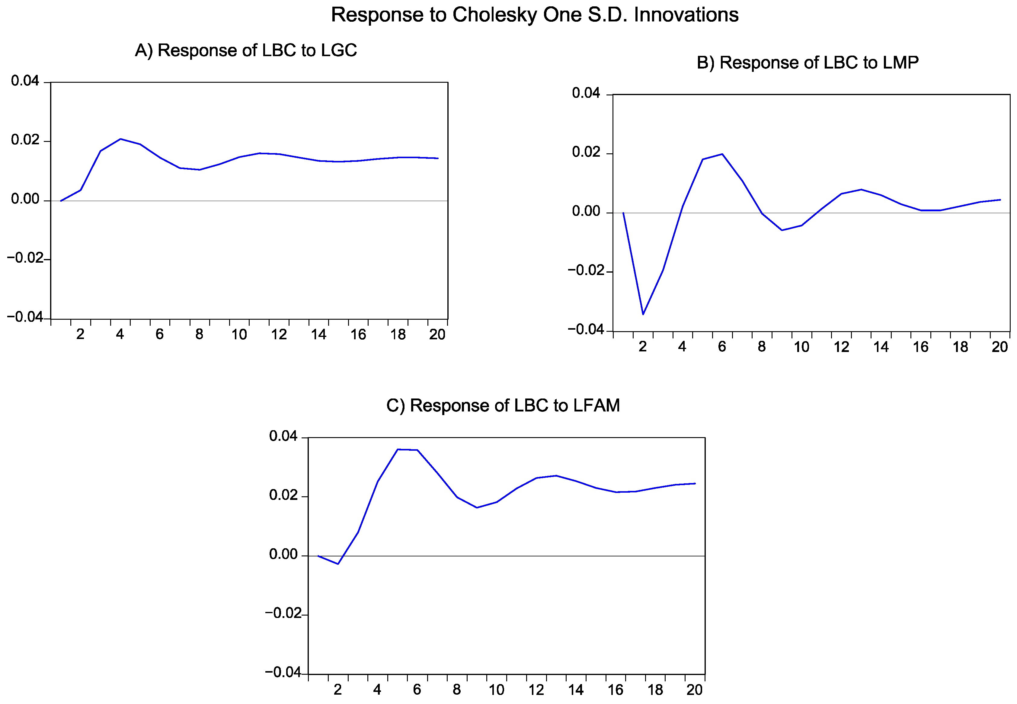
5.4. Impulse Response Function (IRF)

IRF analysis is used to track the impact or movement of a shock on one variable and how that shock will affect that variable or other variable in the present and future. The IRF graph shown in Figure 4 depicts how a variable behaves in reaction to the shock of another variable.
Figure 4A shows the response of the billed amount for the following several periods caused by a shock in GDP. The increase in economic activity level, represented by GDP, will increase the billed amount in the short term by an insignificant amount. In the long run, the billed amount will be stable and do not change. This goes with the result of short and long run.
Figure 4B shows the billed amount response to marginal price: a sudden increase in the marginal water price will decrease the billed amount (the subscriber will tend to reduce his consumption). Although small, the price change has a short effect on the billed amount as it will re-increase after three time periods and then fluctuate over the time horizon until it returns to it is original value; this supports the conclusion of a deficit in supply.
Figure 4C shows the billed amount response to family size; a sudden increase in the family size will lead to a decrease in the billed amount in the short term, and then the billed amount will re-increase after two time periods. Then the water demand will decrease after ten years. The adaptation of water-saving techniques can explain this.
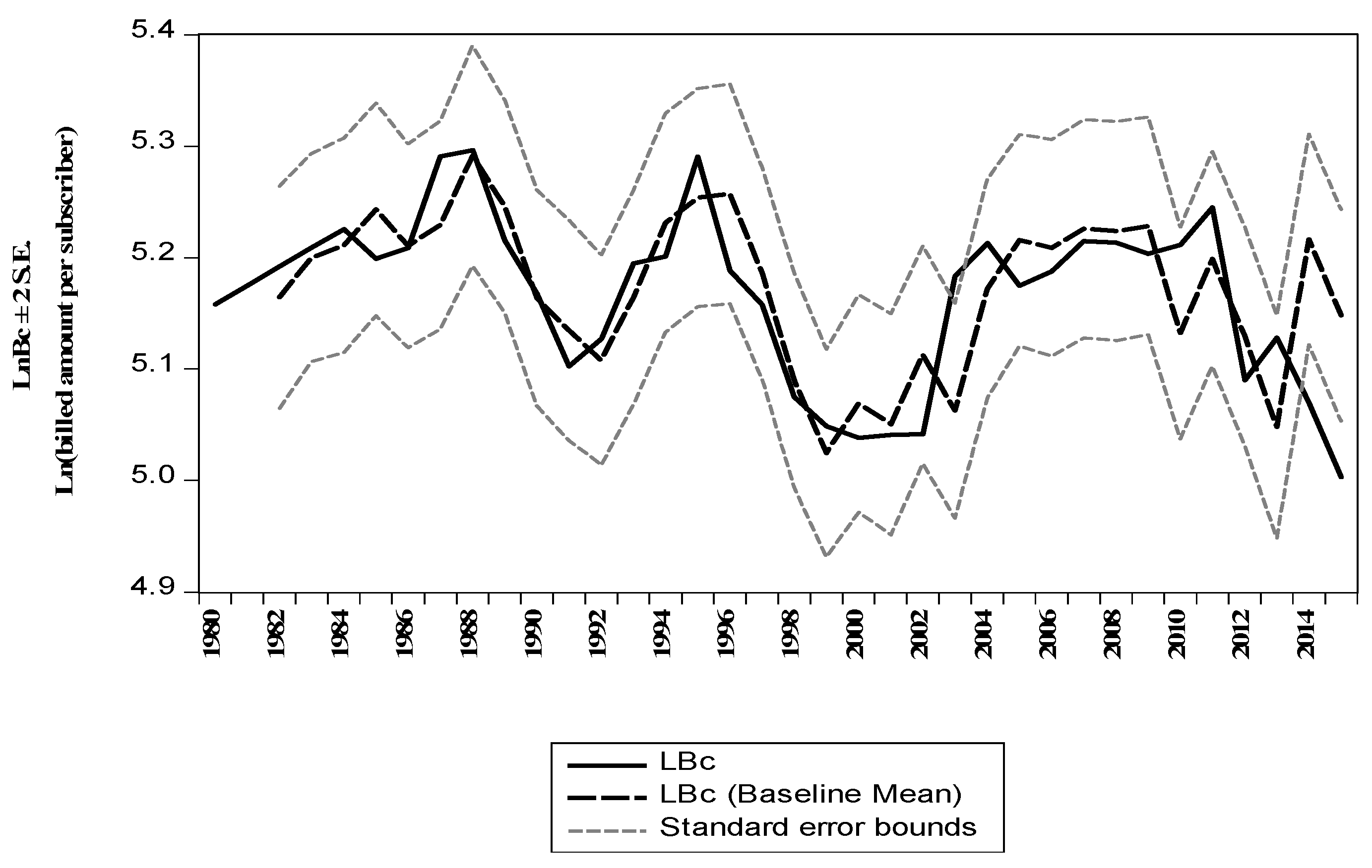
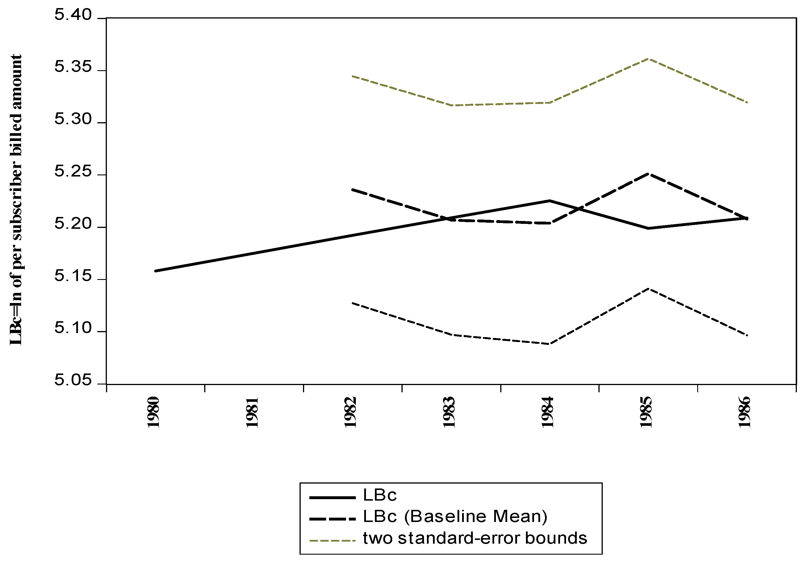
A first model Equation (9) test is accomplished as a within-sample forecast. The forecast is performed using a stochastic simulation and static and dynamic solutions. The results of the sample are shown in Figure 5. As depicted, estimated values are very close to actual values. All estimates are within the two standard error bounds (small dotted lines), indicating a good fit.
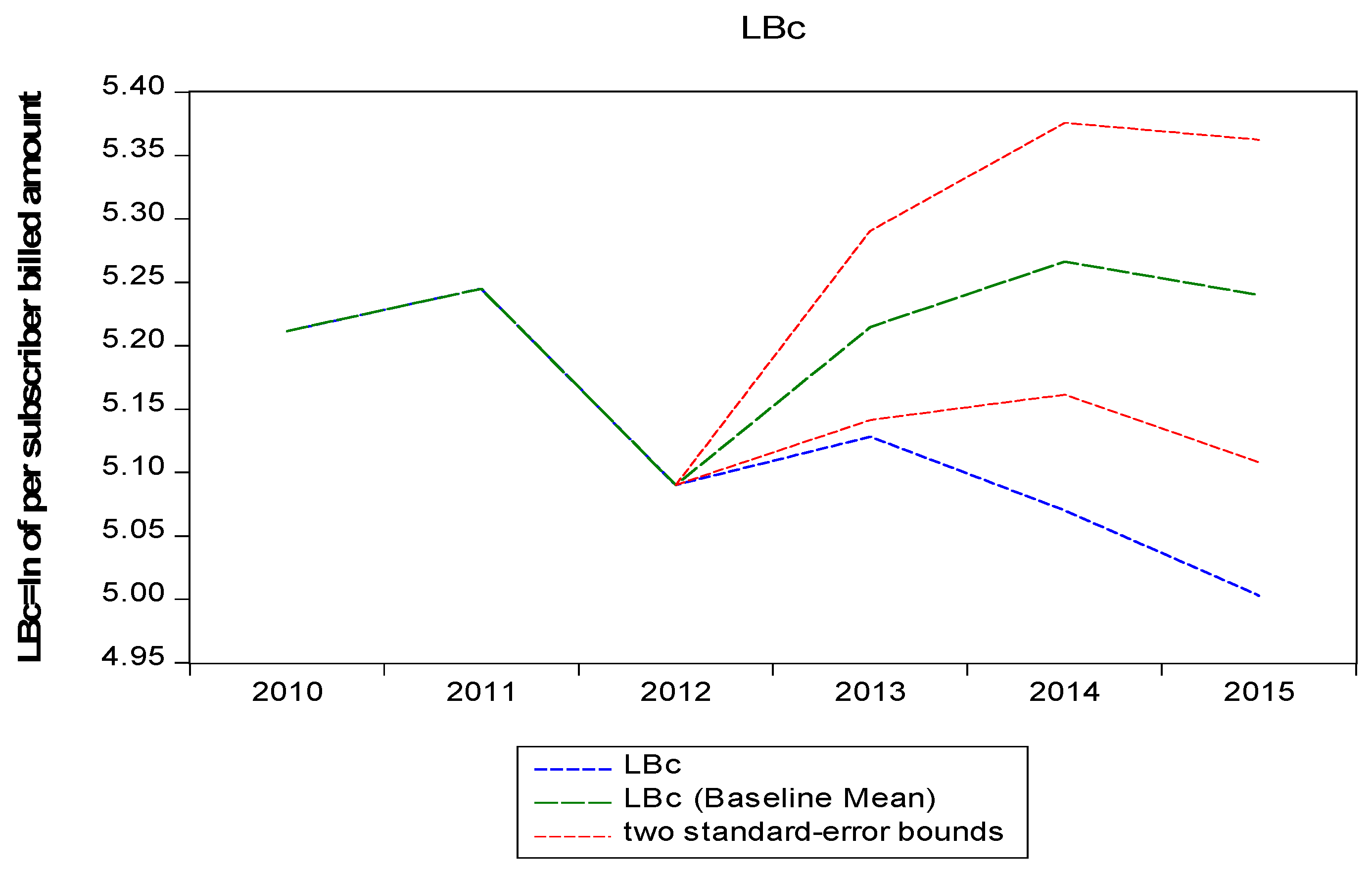
A second, forward, out-of-sample validation is performed using the model presented in Equation (9) and the leftover observations for 2013–2015. The results are shown in Figure 6. Again, forecasted values are within the two standard error bounds and close to the actual values. This confirms the good fit of the model. Similarly, a backward forecast is performed for the years 1980–1983. The prediction uses a VECM (from 1984–2015). The estimation results are shown in Figure 7. They confirm the good fit.

6. Conclusions

The study conducted in the Amman region used data to develop a Vector Error Correction Model with Exogenous Variables (VECMX) to estimate residential water consumption. The model employed various techniques to assess the stationarity of the time series, and after validation, it demonstrated its ability to accurately represent the dynamics of water usage per user.
Water demand for short and long terms is inelastic and minimally responds to price increases; a 1% price rise results in a 0.796% decrease in water use in the short term and a 0.306% decrease in the long term; this aligns with existing research on water demand elasticity in water-scarce regions. Therefore, relying solely on price-based demand management strategies may not be effective.
Water demand is not affected by changes in income levels, whether short or long-term. This finding is consistent with other studies on water demand elasticity. This is particularly evident when water bills are a small percentage of individual income, like in Amman, due to low water prices. Additionally, water scarcity can limit consumption irrespective of income levels. Hence, income-based water demand management strategies are unlikely to be effective in regions with low water pricing and water scarcity, like Amman.
The study shows that in water-scarce regions like Amman, a 1% increase in water supply leads to a proportional increase of 0.682% in per capita water demand. Even minor improvements in the water supply system can result in an increase in water usage, indicating dissatisfaction with the current water demand. To manage water resources effectively, policies should prioritize maintaining and improving the water supply system and controlling non-revenue water.
In the short term, a larger family size reduces per capita water consumption due to economies of scale. As the family size increases by 1%, the billed water demand will decrease by 0.619%. However, in the long term, family size increases water demand. A 1% increase in family size is predicted to increase water demand by 0.36%. To ensure efficient water management, it is crucial to develop strategies that respond to changes in population and promote water-saving technologies and practices in households.
Water consumption correlates positively with days over 30 °C but has no short-term impact on demand. This aligns with most water-scarce literature.
The model can help Amman Water Utility design policies for future water demand. It can also be customized by other utilities in Jordan and other nations to forecast household water demand. Further research can include new variables and extending the model’s application to other regions to improve global water management.

Author Contributions

Conceptualization, D.B.T., A.Q.J. and R.I.; methodology, D.B.T.; software, D.B.T.; validation, D.B.T. and A.Q.J.; formal analysis, D.B.T.; investigation, D.B.T.; resources, D.B.T., A.Q.J. and R.I.; data curation, D.B.T.; writing—original draft preparation, D.B.T.; writing—review and editing, D.B.T.; visualization, D.B.T., A.Q.J. and R.I. All authors have read and agreed to the published version of the manuscript.

Funding

This research received no external funding.

Institutional Review Board Statement

Not applicable.

Informed Consent Statement

Not applicable.

Data Availability Statement

Data is unavailable due to privacy or ethical restrictions.

Conflicts of Interest

The authors declare no conflict of interest.

References

  1. Fawzi, M.; Al Ajlouni, M.I. Water Safety Plan Resources in Jordan Quantity and Quality. Preprints 2021, 2021070709. [Google Scholar] [CrossRef]
  2. Younis, H.I.; Kizhisseri, M.I.; Mohamed, M.M. Forecasting Future Water Demands for Sustainable Development in Al-Ain City, United Arab Emirates. Water 2023, 15, 3800. [Google Scholar] [CrossRef]
  3. Alhusban, A.A.; Alhusban, S.A. Re-locating the identity of Amman’s city through the hybridization process. J. Place Manag. Dev. 2020, 14, 81–113. [Google Scholar] [CrossRef]
  4. Farhan, Y.; Al-Shawamreh, S. Impact of Rapid Urbanization and Changing Housing Patterns on Urban Open Public Spaces of Amman, Jordan: A GIS and RS Perspective. J. Environ. Prot. 2019, 10, 57–79. [Google Scholar] [CrossRef]
  5. Borgomeo, E.; Fawzi, N.A.; Hall, J.W.; Jägerskog, A.; Nicol, A.; Sadoff, C.W.; Salman, M.; Santos, N.; Talhami, M. Tackling the Trickle: Ensuring Sustainable Water Management in the Arab Region. Earth’s Future 2020, 8, e2020EF001495. [Google Scholar] [CrossRef]
  6. Sandeep, V.; Khandekar, A.; Kumar, M. Water Supply, Urbanization and Climate Change. In Resilience, Response, and Risk in Water Systems; Springer: Singapore, 2020. [Google Scholar] [CrossRef]
  7. De Wrachien, D.; Schultz, B.; Goli, M.B. Impacts of population growth and climate change on food production and irrigation and drainage needs: A world-wide view. Irrig. Drain. 2021, 70, 981–995. [Google Scholar] [CrossRef]
  8. Kilic, Z. The Impact of Climate Change on Water Resources. Int. J. Sci. Technol. Res. 2020, 6. [Google Scholar] [CrossRef]
  9. Al-Najjar, F.O.; Al-Karablieh, E.; Al-Karablieh, E.K.; Salman, A. Residential Water Demand Elasticity in Greater Amman Area. 2011. Available online: https://www.researchgate.net/publication/259278881 (accessed on 29 December 2023).
  10. Salman, A.; Al-karablieh, E. Socioeconomic factors influencing the households water demand function in Socioeconomic Factors Influencing the Household Water Demand Function in Jordan. In Proceedings of the International Conference: Integrated Water Resource Management and Challenges of the Sustainable Development, Marrakech, Morocco, 23–25 May 2006. [Google Scholar]
  11. Tabieh, M.; Salman, A.; Al-karablieh, E.; Al-qudah, H. The Residental Water Demand Function in Amman-Zarka Basin in Jordan. Wulfenia J. 2012, 19, 324–333. [Google Scholar]
  12. Arbués, F.; García-Valiñas, M.Á.; Martínez-Espiñeira, R. Estimation of residential water demand: A state-of-the-art review. J. Socio-Econ. 2003, 32, 81–102. [Google Scholar] [CrossRef]
  13. Niknam, A.; Zare, H.K.; Hosseininasab, H.; Mostafaeipour, A.; Herrera, M. A Critical Review of Short-Term Water Demand Forecasting Tools—What Method Should I Use? Sustainability 2022, 14, 5412. [Google Scholar] [CrossRef]
  14. Martínez-Espiñeira, R. An estimation of residential water demand using co-integration and error correction techniques. J. Appl. Econ. 2007, 10, 161–184. [Google Scholar] [CrossRef]
  15. Al-Dhowalia, K.H. Modeling Municipal Water Demand Using Box-Jenkins Technique. J. King Abdulaziz Univ. Eng. 1996, 8, 61–71. [Google Scholar] [CrossRef]
  16. Gam, I.; Aïcha, R.; Rejeb, J. Water Demand, Distribution and Consumption Forecasting: Case of Tunisia. Int. J. Adv. Manag. Econ. 2013, 2, 137–146. [Google Scholar]
  17. Martinez-Espiñeira, R. Residential water demand in the Northwest of Spain. Environ. Resour. Econ. 2002, 21, 161–187. [Google Scholar] [CrossRef]
  18. Garcia, J.; Salfer, L.R.; Kalbusch, A.; Henning, E. Identifying the drivers of water consumption in single-family households in Joinville, Southern Brazil. Water 2019, 11, 1990. [Google Scholar] [CrossRef]
  19. House-Peters, L.A.; Chang, H. Urban water demand modeling: Review of concepts, methods, and organizing principles. Water Resour. Res. 2011, 47, e9624. [Google Scholar] [CrossRef]
  20. Worthington, A.; Hoffmann, M. A State of the Art Review of Residential Water Demand Modelling; School of Accounting and Finance Working Paper; University of Wollongong: Wollongong, NSW, Australia, 2006. [Google Scholar] [CrossRef]
  21. Puri, R.; Maas, A. Evaluating the Sensitivity of Residential Water Demand Estimation to Model Specification and Instrument Choices. Water Resour. Res. 2020, 56, e2019WR026156. [Google Scholar] [CrossRef]
  22. Mitrică, B.; Bogardi, I.; Mitrică, E.; Mocanu, I.; Minciună, M. A forecast of public water scarcity on Leu-Rotunda Plain, Romania, for the end of the 21st century. Nor. Geogr. Tidsskr. 2017, 71, 12–29. [Google Scholar] [CrossRef]
  23. Ajbar, A.H.; Ali, E.M. Prediction of municipal water production in touristic Mecca City in Saudi Arabia using neural networks. J. King Saud. Univ. Eng. Sci. 2015, 27, 83–91. [Google Scholar] [CrossRef]
  24. Ghiassi, M.; Zimbra, D.K.; Saidane, H. Urban Water Demand Forecasting with a Dynamic Artificial Neural Network Model. J. Water Resour. Plan. Manag. 2008, 134, 138–146. [Google Scholar] [CrossRef]
  25. Awad, M.; Zaid-Alkelani, M. Prediction of Water Demand Using Artificial Neural Networks Models and Statistical Model. Int. J. Intell. Syst. Appl. 2019, 11, 40–55. [Google Scholar] [CrossRef]
  26. Alsumaiei, A.A. Short-term forecasting of monthly water consumption in hyper-arid climate using recurrent neural networks. J. Eng. Res. 2021, 9, 57–69. [Google Scholar] [CrossRef]
  27. Moretti, M.; Fiorillo, D.; Guercio, R.; Giugni, M.; De Paola, F.; Uberti, G.S.D. A Preliminary Analysis for Water Demand Time Series. Environ. Sci. Proc. 2022, 21, 7. [Google Scholar] [CrossRef]
  28. Ristow, D.C.M.; Henning, E.; Kalbusch, A.; Petersen, C.E. Models for forecasting water demand using time series analysis: A case study in southern Brazil. J. Water Sanit. Hyg. Dev. 2021, 11, 231–240. [Google Scholar] [CrossRef]
  29. Tripathi, A.; Kaur, S.; Sankaranarayanan, S.; Narayanan, L.K.; Tom, R.J. Water demand prediction for housing apartments using time series analysis. Int. J. Intell. Inf. Technol. 2019, 15, 57–75. [Google Scholar] [CrossRef]
  30. Usman, M.; Loves, L.; Russel, E.; Ansori, M.; Warsono, W.; Widiarti, W.; Wamiliana, W. Analysis of Some Energy and Economics Variables by Using VECMX Model in Indonesia. Int. J. Energy Econ. Policy 2022, 12, 91–102. [Google Scholar] [CrossRef]
  31. Candelieri, A. Clustering and support vector regression for water demand forecasting and anomaly detection. Water 2017, 9, 224. [Google Scholar] [CrossRef]
  32. Bai, Y.; Wang, P.; Li, C.; Xie, J.; Wang, Y. A multi-scale relevance vector regression approach for daily urban water demand forecasting. J. Hydrol. 2014, 517, 236–245. [Google Scholar] [CrossRef]
  33. Zubaidi, S.L.; Al-Bugharbee, H.; Ortega-Martorell, S.; Gharghan, S.K.; Olier, I.; Hashim, K.S.; Al-Bdairi, N.S.S.; Kot, P. A Novel Methodology for Prediction Urban Water Demand by Wavelet Denoising and Adaptive Neuro-Fuzzy Inference System Approach. Water 2020, 12, 1628. [Google Scholar] [CrossRef]
  34. Chen, G.; Long, T.; Bai, Y.; Zhang, J. A Forecasting Framework Based on Kalman Filter Integrated Multivariate Local Polynomial Regression: Application to Urban Water Demand. Neural Process. Lett. 2019, 50, 497–513. [Google Scholar] [CrossRef]
  35. Nasseri, M.; Moeini, A.; Tabesh, M. Forecasting monthly urban water demand using Extended Kalman Filter and genetic programming. Expert. Syst. Appl. 2011, 38, 7387–7395. [Google Scholar] [CrossRef]
  36. Peña-Guzmán, C.; Melgarejo, J.J.; Prats, D. Forecasting Water Demand in Residential, Commercial, and Industrial Zones in Bogotá, Colombia, Using Least-Squares Support Vector Machines. Math. Probl. Eng. 2016, 2016, 5712347. [Google Scholar] [CrossRef]
  37. Engle, R.F.; Granger, C.W.J. Co-Integration and Error Correction: Representation, Estimation, and Testing. Econometrica 1987, 55, 251–276. [Google Scholar] [CrossRef]
  38. Seo, B. Statistical inference on cointegration rank in error correction models with stationary covariates. J. Econom. 1998, 85, 339–385. [Google Scholar] [CrossRef]
  39. Reynaud, A. Modelling Household Water Demand in Europe; JRC Technical Reports; European Commission: Brussels, Belgium, 2015. [Google Scholar] [CrossRef]
  40. Sebri, M. A meta-analysis of residential water demand studies. Environ. Dev. Sustain. 2014, 16, 499–520. [Google Scholar] [CrossRef]
  41. Nauges, C.; Whittington, D. Estimation of water demand in developing countries: An overview. World Bank. Res. Obs. 2009, 25, 263–294. [Google Scholar] [CrossRef]
  42. Worthington, A.C.; Hoffman, M. An empirical survey of residential water demand modelling. J. Econ. Surv. 2008, 22, 842–871. [Google Scholar] [CrossRef]
  43. Dalhuisen, J.M.; Florax, R.J.G.M.; de Groot, H.L.F.; Nijkamp, P. Price and income elasticities of residential water demand: A meta-analysis. Land. Econ. 2003, 79, 292–308. [Google Scholar] [CrossRef]
  44. Espey, M.; Espey, J.; Shaw, W.D. Price Elasticity of Residential Demand for Water: A Meta-analysis. Water Resour. Res. 1997, 33, 1369–1374. [Google Scholar] [CrossRef]
  45. Kotagama, H.; Zekri, S.; Al Harthi, R.; Boughanmi, H. Demand function estimate for residential water in Oman. Int. J. Water Resour. Dev. 2017, 33, 907–916. [Google Scholar] [CrossRef]
  46. Musolesi, A.; Nosvelli, M. Long-run water demand estimation: Habits, adjustment dynamics and structural breaks. Appl. Econ. 2010, 43, 2111–2127. [Google Scholar] [CrossRef]
  47. Musolesi, A.; Nosvelli, M. Dynamics of residential water consumption in a panel of Italian municipalities. Appl. Econ. Lett. 2007, 14, 441–444. [Google Scholar] [CrossRef]
  48. Nauges, C.; Thomas, A. Long-run Study of Residential Water Consumption. Environ. Resour. Econ. 2003, 26, 25–43. [Google Scholar] [CrossRef]
  49. Arbués, F.; Barberán, R.; Villanúa, I. Price impact on urban residential water demand: A dynamic panel data approach. Water Resour. Res. 2004, 40, W11402. [Google Scholar] [CrossRef]
  50. Barberán, R.; Arbués, F. Equity in domestic water rates design. Water Resour. Manag. 2009, 23, 2101–2118. [Google Scholar] [CrossRef]
  51. Arbués, F.; Villanúa, I.; Barberán, R. Household size and residential water demand: An empirical approach. Aust. J. Agric. Resour. Econ. 2010, 54, 61–80. [Google Scholar] [CrossRef]
  52. Telfah, D.B.; Louzi, N.; AlBashir, T.M. Water demand time series forecast by autoregressive distributed lag (ARDL) co-integration model. J. Water Land Dev. 2021, 50, 195–206. [Google Scholar] [CrossRef]
  53. Cabral, M.; Mamade, A.; Loureiro, D.; Amado, C.; Covas, D. Modeling the effect of weather conditions on urban water demand in multiple network areas: A practical approach to improve monthly and seasonal operation. J. Water Supply Res. Technol. AQUA 2016, 65, 612–625. [Google Scholar] [CrossRef]
  54. Romano, G.; Salvati, N.; Guerrini, A. Estimating the determinants of residential water demand in Italy. Forests 2014, 5, 2929–2945. [Google Scholar] [CrossRef]
  55. Maidment, D.R.; Miaou, S. Daily Water Use in Nine Cities. Water Resour. Res. 1986, 22, 845–851. [Google Scholar] [CrossRef]
  56. Lavín, F.A.V.; Hernandez, J.I.; Ponce, R.D.; Orrego, S.A. Functional forms and price elasticities in a discrete continuous choice model of the residential water demand. Water Resour. Res. 2017, 53, 6296–6311. [Google Scholar] [CrossRef]
  57. Nieswiadomy, M.L.; Molina, D.J. A Note on Price Perception in Water Demand Models. Land Econ. 1991, 67, 352. [Google Scholar] [CrossRef]
  58. Nataraj, S.; Hanemann, W.M. Does marginal price matter? A regression discontinuity approach to estimating water demand. J. Environ. Econ. Manag. 2011, 61, 198–212. [Google Scholar] [CrossRef]
  59. Dickey, D.A.; Fuller, W.A. Distribution of the Estimators for Autoregressive Time Series with a Unit Root. J. Am. Stat. Assoc. 1979, 74, 427–431. [Google Scholar] [CrossRef]
  60. Johansen, S. Estimation and Hypothesis Testing of Cointegration Vectors in Gaussian Vector Autoregressive Models. Econometrica 1991, 59, 1551–1580. [Google Scholar] [CrossRef]
  61. Johamen, S.; Jtiselius, K. Maximum Likelihood Estimation and Inference on Cointegration—With Application to the Demand for Money. Oxf. Bull. Econ. Stat. 1990, 52, 169–210. [Google Scholar]
  62. Hui, E.C.M.; Yue, S. Housing price bubbles in Hong Kong, Beijing and Shanghai: A comparative study. J. Real Estate Financ. Econ. 2006, 33, 299–327. [Google Scholar] [CrossRef]
  63. Granger, C.W.G.; Newbold, P. Spurious regressions in econometrics. J. Econom. 1974, 2, 111–120. [Google Scholar] [CrossRef]
  64. Bai, J.; Perron, P. Computation and analysis of multiple structural change models. J. Appl. Econom. 2003, 18, 1–22. [Google Scholar] [CrossRef]
  65. Barberán Ortí, R.; Inmaculada, V.M.; Arbués Gracia, F. Water Price Impact on Residential Water Demand in Zaragoza City. A Dynamic Panel Data Approach. In Proceedings of the 40th Congress of the European Regional Science Association: “European Monetary Union and Regional Policy”, Barcelona, Spain, 29 August–1 September 2000; European Regional Science Association (ERSA): Louvain-la-Neuve, Belgium, 2000. Available online: http://hdl.handle.net/10419/114831 (accessed on 4 October 2023).
  66. Gaudin, S. Effect of price information on residential water demand. Appl. Econ. 2006, 38, 383–393. [Google Scholar] [CrossRef]
Figure 1. Time series used in the analysis in natural logarithm against years in the horizontal axis of: (a) natural logarithm of Billed amount/capita (LBC) against years; (b) natural logarithm of GDP per capita (LGC) against years (c) natural logarithm of marginal price (LMP) against years (d) natural logarithm of family size (LFam) against years yearly (e) System Input/capita (LIC) against years (f) natural logarithm of The count of days in which the ambient temperature climbed above 30 °C in the year Amman (LT30) against years. Source: Original work created by the author utilizing Eviews software version 12 and model data.
Sustainability 16 02315 g001
Figure 2. Inverse Roots of the Autoregressive Polynomial (VAR).
Sustainability 16 02315 g002
Figure 3. Recursive estimate (CUSUM) of OLS Equation.
Sustainability 16 02315 g003
Figure 4. Impulse Response Function.
Sustainability 16 02315 g004
Figure 5. Within the sample forecast using a stochastic solution type and static dynamics.
Sustainability 16 02315 g005
Figure 6. Forward forecast and validation for observation years 2013, 2014, 2015.
Sustainability 16 02315 g006
Figure 7. Backward forecast and validation for observation years from 1980 to 1983.
Sustainability 16 02315 g007
Table 1. The Impact of Independent Variable Proximity on Dependent Variable.
Independent VariableNotationTiming of Effect on Billed Amount (DV)Variables
Billed amount/capitaBcThe analysis encompasses all prior dynamics of the variable.Endogenous
Marginal PriceMpAccording to the majority of studies, it is deemed insignificant in the short and long term.Endogenous
GDP per capitaGcAccording to the majority of studies, it is deemed insignificant in the short and long term.Endogenous
System Input/capitaIcThe short-run effect is considered to be significant in the majority of the literature.Exogenous
Family sizeFamThe short-run effect is considered to be significant in the majority of the literature.Endogenous
Temperature (The number of days in which temperature exceeded 30 °C)T30Long-term and short-term estimates of its significance are low in most literature on water-scarce regions.Exogenous
Table 2. Series Used (Determinates) and Their Source and Notation.
VariableNotationSource
Billed amount/capita (m3/Yr per capita)BcMIY and WAJ + (calculation)
Marginal Price in 100 * Jordan DinarsMp (Piaster)
System Input per subscriber (m3/year per capita)Ic
Subscriber/family size (number)FamDOS + MIY calculation
GDP per capitaGcCBJ- and DOS
The count of days in which the ambient temperature climbed above 30 °C in the yearT30JMD
* One Jordan Dinars (JD) is equivalent to 1.142 US Dollars. Source: own elaboration based on listed sources.
Table 3. Descriptive Statistics.
LBcLMpLIcLGcLFamLT30
Mean5.1754.0866.9575.8811.8964.708
Median5.1924.1366.9955.9021.8984.691
Maximum5.2964.6337.1256.1062.0235.081
Minimum5.0383.3156.6965.6911.7744.369
Std. Dev.0.0700.3270.1280.1080.0900.143
Skewness(0.529)(0.650)(0.487)(0.008)0.2120.199
Kurtosis1.5532.8071.3101.9771.2473.312
Jarque-Bera2.9602.3753.9272.7444.2420.352
Probability0.2280.3050.1400.2540.1200.839
Sum174.98134.84198.27229.5865.46155.37
Sum Sq. Dev.0.6893.4231.2720.5220.7530.655
Observations333333333333
Table 4. Augmented Dickey-Fuller test statistics lag length according to Schwarz info Criterion of max lag = 8, and Individual Time Series Stationarity test results (sample 1980–2012) Source: own study.
VariableVariable (Regressor)
Ln(Bc)Ln(Mp)Ln(Ic)Ln(Gc)Ln(Fam)Ln(T30)
t-statPropt-statPropt-statPropt-statPropt-statPropt-statProp
LevelIntercept−2.280.18−1.860.35−1.560.49−1.920.32−1.480.53−4.360.00
Trend and Intercept−2.380.38−3.170.11−2.520.32−2.870.19−0.620.97−6.350.00
None−0.240.592.821.00−0.470.51−0.510.49−0.880.331.580.97
First DifferenceIntercept−4.350.00−4.930.00−5.620.00−4.070.00−4.220.00−6.230.00
Trend and Intercept−4.260.01−5.040.00−5.570.00−4.190.01−4.410.01−6.270.00
None−4.450.00−3.990.00−5.670.00−4.150.00−4.220.00−5.830.00
Results of Stationarity at both 5% and 1%. Yes = Stationary, No = Non stationary
VariableLn(Bc)Ln(Mp)Ln(Ic)Ln(Gc)Ln(Fam)Ln(T30)
5%1%5%1%5%1%5%1%5%1%5%1%
LevelInterceptNoNoNoNoNoNoNoNoNoNoYesYes
Trend and InterceptNoNoNoNoNoNoNoNoNoNoYesYes
NoneNoNoNoNoNoNoNoNoNoNoNoNo
First DifferenceInterceptYesYesYesYesYesYesYesYesYesYesYesYes
Trend and InterceptYesYesYesYesYesYesYesYesYesYesYesYes
NoneYesYesYesYesYesYesYesYesYesYesYesYes
Table 5. Unit root with break test LT30.
Augmented Dickey-Fuller Test Statistict-StatisticProb. *
−5.57066<0.01
Test critical values:1% level−4.33515
5% level−3.7297
10% level−3.44485
* Perron (1989, 1993) asymptotic one-sided p-values (lambda = 0.424242).
Table 6. Results of Lag Length Criteria Testing.
LagLogLLRFPEAICSCHQ
0109.8091NA1.02×10−8−7.053942−6.867115−6.994174
1226.3738194.2744 *1.26×10−11 *−13.75825 *−12.82412 *−13.45941 *
2236.257513.837272.02×10−11−13.35050−11.66907−12.81260
3251.091316.811592.58×10−11−13.27275−10.84401−12.49578
* indicates lag order selected by the criterion.
Table 7. Results of Five models of the Johansen Co-integration test.
Data Trend:NoneNoneLinearLinearQuadratic
Test TypeNo InterceptInterceptInterceptInterceptIntercept
No TrendNo TrendNo TrendTrendTrend
Trace11111
Max-Eig11111
Table 8. Co-integration test results using Johansen (1991,1995) with Linear deterministic trend.
Unrestricted Co-Integration Rank Test (Trace)
Hypothesized No. of
Co-Integration Equations
EigenvalueTrace Statistic0.05 Critical ValueProb.
None *0.74112767.5870347.856130.0003
At most 10.34183625.6930429.797070.1381
At most 20.30738212.7256915.494710.1253
At most 30.0423091.3401193.8414660.247
Unrestricted Co-integration Rank Test (Maximum Eigenvalue)
HypothesizedEigenvalueMax-Eigen Statistic0.05 Critical ValueProb.
None *0.74112741.8939927.584340.0004
At most 10.34183612.9673521.131620.4552
At most 20.30738211.3855714.264600.1359
At most 30.0423091.3401193.8414660.2470
* denotes rejection of the hypothesis at the 0.05 level.
Table 9. Results of Granger-causality Wald Tests based on the VECM.
Null HypothesesVEC Granger Causality
Chi-SquareChi-Square
Gross domestic product does not Granger-cause the water demand0.7873670.3749
Marginal price does not Granger-cause the water demand22.659470.0000
Family size does not Granger-cause the water demand4.1524950.0416
Model does not Granger-cause the water demand36.560580.0000
Table 10. Long-run elasticities of the VECMX Model.
Variable ρ 0 LBct-1LMpt-1LGct-1LFamt-1
Coefficient18.97510.306195−0.0291−0.360655
Standard Error 0.764360.460681.94222
T-statistic [3.07698][−0.06317][−4.00075]
Probability (%) <5%>5%<5%
Note: LBc = per subscriber yearly billed water amount (m3∙y−1), LMp = marginal Price, LGc = real per capita GDP at basic prices, LFam = Family size.
Table 11. Short-run elasticities of the VECMX Model.
ParameterVariable
CD(LBC(–1))D(LGC(–1))D(LMP(–1))D(LFAM(–1))D(LIC)LT30ResCointEq (α)
Coefficient0.023−0.2010.169−0.796−0.6190.6820.003−0.476813
Standard Error0.0087460.1585010.2021090.1673390.3064570.1147980.0803520.116791
T statistic2.656295−1.2690950.834856−4.758085−2.0186245.9440820.035287−4.082628
Probability (%)0.010.220.410.000.060.000.970.0005
R20.725232
Adjusted R20.633643
F-statistic7.918313
Prob (F-statistic)0.000098
Durbin–Watson stat 1)2.111821
1 Durbin–Watson stat is greater than 2, indicating negative autocorrelation. Values from 0 to less than two positive autocorrelations and values from 2 to 4 indicate negative autocorrelation.
Table 12. Diagnostic tests of the estimated VECMX model.
DiagnosticsStatistics
LM (1)17.474 (0.356)
LM (4)14.503 (0.561)
LM (8)12.56994 (0.704)
White132.5104 (0.661)
Jarque-Bera0.8108 (0.667)
Notes: LM(p) is the Lagrange multiplier test for residual serial correlation with p lag length; White is White’s test for heteroskedasticity; Jarque-Bera is the Jarque Bera test for normality of the residuals; figures in parentheses denote probability values.
Disclaimer/Publisher’s Note: The statements, opinions and data contained in all publications are solely those of the individual author(s) and contributor(s) and not of MDPI and/or the editor(s). MDPI and/or the editor(s) disclaim responsibility for any injury to people or property resulting from any ideas, methods, instructions or products referred to in the content.

