An Empirical Evaluation of a New Heuristic Method for Identifying Safety Improvement Sites on Rural Highways: An Oregon Case Study

Abstract

Road safety is considered one of the fundamental factors for sustainable mobility, which requires establishing effective highway safety management programs and processes. Identifying safety improvement sites (network screening) is a critical step in the state roadway safety programs. The overall effectiveness of these programs largely relies on the robustness of the network screening method in identifying sites with high potential for safety improvements. This study investigates the network screening performance of a new proposed methodology that employs heuristic scoring schemes to account for roadway and roadside characteristics, crash history, and traffic exposure. The new method, originally proposed for use on rural low-volume roads, is simplistic in that it does not require exact and detailed information on traffic and geometric characteristics and can still be applied in the absence of crash data. The performance evaluation is conducted using a sample of 1495 miles of rural two-lane highway segments in Oregon. The effectiveness of the proposed method is assessed using observed crash history and compared to the well-established Empirical Bayes method as a reference. The effect of traffic level on the performance of the proposed method was evaluated using separate analyses for lower and higher traffic volume segments. The study findings indicate that the effectiveness of the proposed method in identifying sites with potential safety improvements is overall high and slightly exceeded that of the more sophisticated and data-intensive Empirical Bayes method. When data were stratified by traffic volume, the proposed method was found to be more effective for lower volume roads; however, the Empirical Bayes method outperformed the proposed method for higher volume roads.

1. Introduction

Highway safety improvement programs (HSIPs) are the primary means for managing safety on the highway system, thus promoting sustainable mobility on the urban and rural highway networks. The Highway Safety Improvement Program (HSIP) is a core federal aid program for states to achieve a significant reduction in fatalities and serious injuries on all public roads. The HSIP requires a data-driven, strategic approach to improving highway safety on all roads, including non-state-owned roads and roads on tribal lands, with a focus on performance [1]. The HSIP is a six-step process including network screening, crash analysis and diagnosis, countermeasure selection, economic appraisal, project prioritization, and safety effectiveness evaluation. The program is outlined in detail in the US Highway Safety Manual [2].

Network screening is a critical step in highway safety improvement programs, which seek to identify sites at the network level that are good candidates for further consideration and investigation for safety improvement. An effective network screening method would lead to identifying sites where potential safety benefits are maximized for better use of the limited safety improvement funds. The traditional methods for network screening are reactive in nature and require the use of extensive crash and traffic data. On the other hand, several proactive approaches have been proposed or used in practice that do not rely solely on crash history and often require data on roadway geometry and roadside characteristics. A major challenge for network screening on rural roads is the lack of access to the required crash, roadway, and traffic data at the network level, especially for roadways that are owned and operated by local agencies.

While HSIPs are applied to both urban and rural highway networks, rural highways pose unique challenges for safety management programs. Specifically, rural roads, which constitute the vast majority of the highway network by length, normally witness a disproportionately high rate of vehicle crashes compared to roads in urban areas. According to the fatality facts 2021, around 40% of traffic fatalities took place in rural areas, although only 20% of people in the U.S. live there, and 32% of all vehicle miles traveled (VMT) occurred in rural areas [3]. These statistics demonstrate the need for improving rural road safety and the requirement to effectively include it in the ongoing state safety improvement programs. A major issue with safety improvement for rural highways is that the crashes on rural and local roads are typically spread over hundreds of miles and are not as densely clustered as crashes in urban areas.

This research seeks to evaluate the performance of a novel yet simplistic network screening method that was tailored for use on rural roadways. The proposed method requires minimal data and technical expertise for implementation which could be valuable for small agencies having limited access to data and/or lacking staff with a traffic safety background. An overview of the proposed method is discussed later in Section 4 of this paper.

2. Literature Review

Numerous network screening techniques have been used in practice or proposed in the literature with each having its strengths and limitations. Some of these techniques are well established in practice, while others have seen limited or no practical implementations to learn about their effectiveness. In this section, the major studies that evaluated the use of the Highway Safety Manual (HSM) safety performance function (SPF) predictive models and the Empirical Bayes (EB) method for network screening are summarized and presented. The HSM, published by the American Association of State Highway Transportation Officials (AASHTO), is the national document and reference for conducting quantitative traffic safety analyses on existing or proposed roadways [2]. Safety Performance Functions are statistical models used to estimate the average crash frequency (predicted number of crashes) for a specific highway type (segments or intersections). The Empirical Bayes method estimates the expected number of crashes using the HSM predicted a number of crashes and the observed number of crashes from crash history.

Kwon et al. [4] evaluated the performance of three network screening methods for detecting high collision concentration locations on highways: Sliding Moving Window (SMW), Peak Searching (PS), and Continuous Risk Profile (CRP). The study assessed the performance of the three methods for segmenting freeway sites to identify high-collision concentration locations. Excess expected average crash frequency was estimated using Empirical Bayes adjustment, considering two sets of Safety Performance Functions (SPFs). Different SPFs and segment definitions were applied to test the robustness of these methods. The estimates from each method were then used to prioritize sites for safety investigation, comparing them with confirmed high collision concentration locations. The input requirements for all three methods are the same. The findings indicated that the CRP method exhibited the lowest false positive rate, accurately identifying sites requiring safety investigation.

A study by Ambrose et al. [5] investigated the difference between network screening results based on multivariate and simple crash prediction models. This study first compared the list of segments using Spearman’s rank correlation coefficient between the two models. Secondly, this study assessed the equality of statistical distributions of potential for safety improvement (PSI) value, which was obtained as a difference between predicted crash frequency and EB estimate. The third comparison was the percentage of segments identified in both lists. The findings suggested that the results from both methods were comparable.

Another study in Brazil [6] presented a comparative analysis of safety performance measures, considering its applicability limitations in a sample of signalized intersections from Fortaleza City, Brazil. The safety performance measures assessed in this study are average crash frequency (ACF), crash rate (CR), Equivalent Property Damage Only (EPDO), Level of Service of Safety (LOSS), Excess Predicted Average Crash Frequency using Safety Performance Functions (SPFs), Expected Average Crash Frequency with EB Adjustments (EB), and Excess Expected Average Crash Frequency with EB Adjustment (EEB). The rank difference between each safety performance measure and the Excess Expected Average Crash Frequency with EB Adjustment (EEB) was used to determine how well each measure ranked the sample intersection. In addition, this study has taken a temporal analysis based on the consistency of safety performance measures during subsequent time periods. The outcome indicated that the most comprehensive safety performance measure, EEB, and the basic safety performance measures, like crash frequency and crash rate, reasonably matched.

The effectiveness of several network screening techniques was examined in an Italian study [7] using a set of criteria. These included reliability in detecting hazardous sites over a period, efficiency in finding sites with poor safety performance, and consistency in ranking. The potential for improvements (PFI) was examined along with the crash frequency, equivalent property damage only (EPDO), crash rate, proportion method, and EB estimates for total and severe crash rates. The evaluation criteria included site consistency, method consistency, total rank differences, and total score tests. This analysis used crash data from an Italian highway and found that the EB method outperformed all other approaches investigated in this study. A different Italian study [8] used simulated data to evaluate the effectiveness of various hotspot identification techniques. A Monte Carlo simulation was used to produce theoretical crash data similar to empirical data, and the data were used to define a priori hazardous sites and, therefore, to assess whether a method could correctly identify such sites. This study assessed the estimated EB, the potential for safety improvement (PSI), observed crash frequency, and crash rate. The EB and PSI methods outperformed the crash frequency and crash rate methods in this study’s identification of high crash locations.

Al-Kaisy and Huda [9] investigated the Empirical Bayes method application on low-volume rural roads. The study found that using the Highway Safety Manual (HSM) EB method, the expected number of crashes for the study sample was reasonably close to the observed number of crashes over the 10-year study period. The study also concluded that it could be very effective to use network screening methods that rely primarily on risk factors for low-volume road networks in a region where accurate and reliable crash data are not available.

A Federal Highway Administration (FHWA) study [10] examined four network screening techniques to identify places with the most potential for safety improvements. The four performance measures included crash frequency, crash rate, EB expected crashes, and EB excess expected crashes—all for the fatal and non-fatal injury severity levels. Utilizing intersection data from New Hampshire, the study tracked the safety management process from network screening to economic analysis. This study analyzed the overall economic benefit and benefit–cost ratio for each of the four techniques. The list of sites with the most significant overall economic benefit and the highest return on investment was generated using the EB excess expected measure and the EB expected measure, respectively.

This section summarized several studies that investigated the performance of network screening methods in the context of the Highway Safety Manual predictive models and the EB method. Specifically, the methods encompass the predicted number of crashes using SPFs, the EB expected number of crashes, and other derivative measures such as the potential for safety improvement (PSI) and EB excess expected crashes. Overall, the studies highlighted the effectiveness of the different network screening methods in identifying sites for safety improvements. However, despite the effectiveness of these methods, their implementation requires extensive crash, traffic and roadway data that may not be accessible to agency staff, particularly those working for local agencies lacking access to detailed databases and technical expertise.

3. Study Motivation

The objective of this study is to evaluate the performance of a novel yet simplistic network screening method that was tailored for use on rural roadways. Rural highways present unique challenges regarding their physical characteristics, travel patterns, and safety risks, often exacerbated by limited access to data and technical expertise for roads managed by local agencies. Specifically, local agencies often lack access to detailed databases and do not have safety engineers among their staff. A rather simplistic method for network screening was developed and proposed for use to address these challenges. However, no evaluation was performed to have a better understanding of the strengths and limitations of the proposed method. Such evaluation is important for making informed decisions about the implementation of the proposed network screening method. Therefore, the major motivation behind this research was to examine the performance of the proposed network screening method that may prove valuable for network screening applications on rural road networks. Effective network screening methods should contribute to successful safety management programs and help promote sustainable mobility on the highway system by reducing the number of crashes, fatalities, and injuries.

4. Overview of Proposed Screening Method

The proposed network screening method uses two heuristic scoring schemes for intersections and roadway segments on rural two-lane highways independently. The Highway Safety Manual (HSM) [2], the nation’s preeminent manual for conducting quantitative safety analyses, was largely the basis for developing the proposed scoring schemes. Using these schemes, an individual site in a network obtains a score that is a function of roadway and roadside characteristics, crash history, and traffic exposure during the analysis period. The proposed scoring scheme for highway segments is shown in

Table 1. Proposed scoring scheme for roadway segments [12,13].

Safety Related Questions	If Yes, Add:
Risk Factors
Total Width (TD)
TD ≤ 20 ft?	7
20 ft < TD ≤ 24 ft?	4
Horizontal curve [Radius (R)]
Flatter curve (R ≥ 300 ft)	30
Sharper curve (R < 300 ft)	60
Grade steeper than 4%?	3
Six or more driveways per mile?	5
Side slope steeper than 1 V:3 H?	4
Fixed objects within 15 ft of travel lane?	4
Unpaved road?	14
Poor pavement condition? (Rutting, potholes, etc.)	7
Crash History Available?
Number of fatal or serious injury crashes (N1)	N1 × 80
Number of other crashes (N2)	N2 × 5
Relative Risk Compound Scores (RRCS)
Speed ≥ 50 mph?	RRCS × 1.25
Got Annual Daily Traffic (ADT)?
ADT ≤ 300	RRCS × 1.0
300 < ADT ≤ 600	RRCS × 3.0
600 < ADT ≤ 1000	RRCS × 5.0
ADT ≥ 1000	RRCS × 7.0
Global Risk Score (GRS)

. Scores for roadway and roadside characteristics are determined depending on the existence of specific road elements (including horizontal curvature, gradient, roadside fixed objects, roadside slope, driveway density, and the total width of the road). Horizontal curves are those curved sections of highways associated with changes in the direction of the road. The radius of the horizontal curve (an indicator of curve sharpness) is used to provide the score for this road characteristic. A roadside fixed object refers to the presence of non-breakaway fixed objects like trees, utility poles, traffic signs, or any hazardous object within 15 feet from the edge of travel lanes. The side slope is defined as the slope of the cut or fill expressed as the ratio of vertical distance to horizontal distance. The scoring scheme assigns a score for side slopes steeper than 1 V:3 H, also known as non-traversable side slopes. The total width of the road is the sum of lane width and shoulder width. The driveway density refers to the concentration or frequency of driveways (access points) along a specific roadway segment expressed as the number of driveways per mile. The scores in the proposed scheme were developed using the crash modification factors (CMFs) for rural two-lane roadways that are supplied in the HSM, published in the CMFs clearinghouse maintained by the Federal Highway Administration [11], or other CMFs reported in published research. The scores assigned to observed crashes were mainly selected to ensure that sites with one or more fatal or serious injury crashes receive further consideration/review for potential safety improvements regardless of the risk factors present. The score assigned to fatal and serious injury crashes is large enough to cause these sites to make it to the priority list of sites. The property-damage-only (PDO) crashes were assigned a weight that is in proportion to the weight assigned to fatal and serious injury crashes (fatal to PDO proportion is 1:16 versus the typical range of 1:15 to 1:25). The proposed screening method also accounts for traffic exposure. The method assigns a multiplier (multiplicative factor) to adjust the relative risk score based on traffic level. These multipliers were derived using the HSM safety performance functions (SPFs) for rural two-lane highways. Specifically, traffic volumes representing volume ranges in the scoring scheme were used in the safety performance function, and the proportions of the resulting number of crashes were used to derive the multipliers.

Upon systemically applying the proposed scoring schemes to all sites that are part of the roadway network, a list of high-priority sites (ranked from highest to lowest scores) can be established and used for further investigation and potential safety treatments. The focus of the current research is on roadway segments, given the availability of data required for this investigation. The framework of the proposed scoring scheme for rural intersections is very similar to the one for roadway segments discussed in this section. However, it is not provided in this section for space constraints, and interested readers are encouraged to check reference [12] for details.

5. Study Area

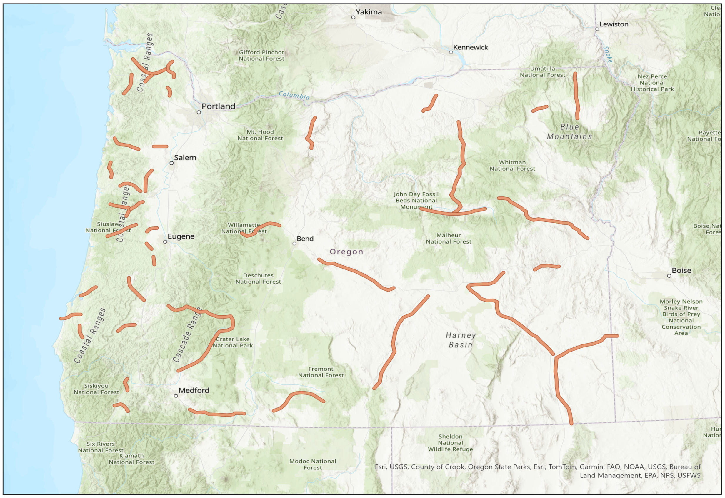
The study area for this research included the state-owned two-lane rural roadway network in the state of Oregon. The state of Oregon was selected in this study for its diverse terrain and area character and for considerations related to data availability and accessibility. A total roadway segment sample of around 1495 miles was used in this investigation to ensure adequate geographic coverage. The study sample included roadways from different parts of the state, as shown in Figure 1. In general, roadways in the eastern part of the state run in flatter terrain with less restrictive alignment, while those in the western part of the state run in mountainous terrain with more restrictive alignment (winding routes, sharp radii, etc.).

6. Data Collection and Processing

All state-owned rural two-lane roads were identified using online geographic information system (GIS) data [14]. The focus was on state-owned roadways for considerations related to data availability and accessibility. Then, selections were made from the results to arrive at the target sample considering geographical coverage. Data were collected for roadway segments using 0.05-mile increments to ensure that data would capture all changes in the physical characteristics of the roadway, thus eliminating the possibility of missing significant differences between consecutive observation points. All segments in the study sample had a posted speed limit of 55 mph. Intersections were not included in the study sample. Intersections and 0.05-mile segments along upstream and downstream approaches were excluded from the dataset.

The Oregon Department of Transportation (ODOT) online databases and video logs were used to identify and compile traffic, roadway geometry, roadside and crash data [15,16]. The roadway geometric data consisted of lane type and width, shoulder type and width, horizontal curve presence and direction, degree of curvature, length of the horizontal curve, spiral curve presence and length, vertical curve presence and type, grade, and length of vertical curve taken from the online database. Roadside characteristics comprised driveway density, side slope ratings, and fixed object ratings taken from ODOT video logs at 0.05-mile resolution.

Crash data from 2011 to 2020 (10 years) were collected for the study sample using the ODOT online database. Data on more than 20 individual crash characteristics—including crash location, road character, impact location, traffic control, crash type, crash severity, vehicle type, and weather condition—were collected and combined with the geometric and roadside database, forming an integrated dataset for analysis.

Traffic data for 10 years (2011–2020) were also collected separately. The ODOT online records were checked to make sure no major changes to roadway geometry happened on the original study sample during the study period [17]. Furthermore, the original study sample was shared with the Oregon DOT personnel to learn about changes that may have taken place in any of the sample segments. The information received from the agency confirmed that there were no changes for the study period.

To maintain the integrity of the analysis, any roadway segment lacking or missing essential data was excluded from the total sample to eliminate any potential impact on study results.

Segmentation

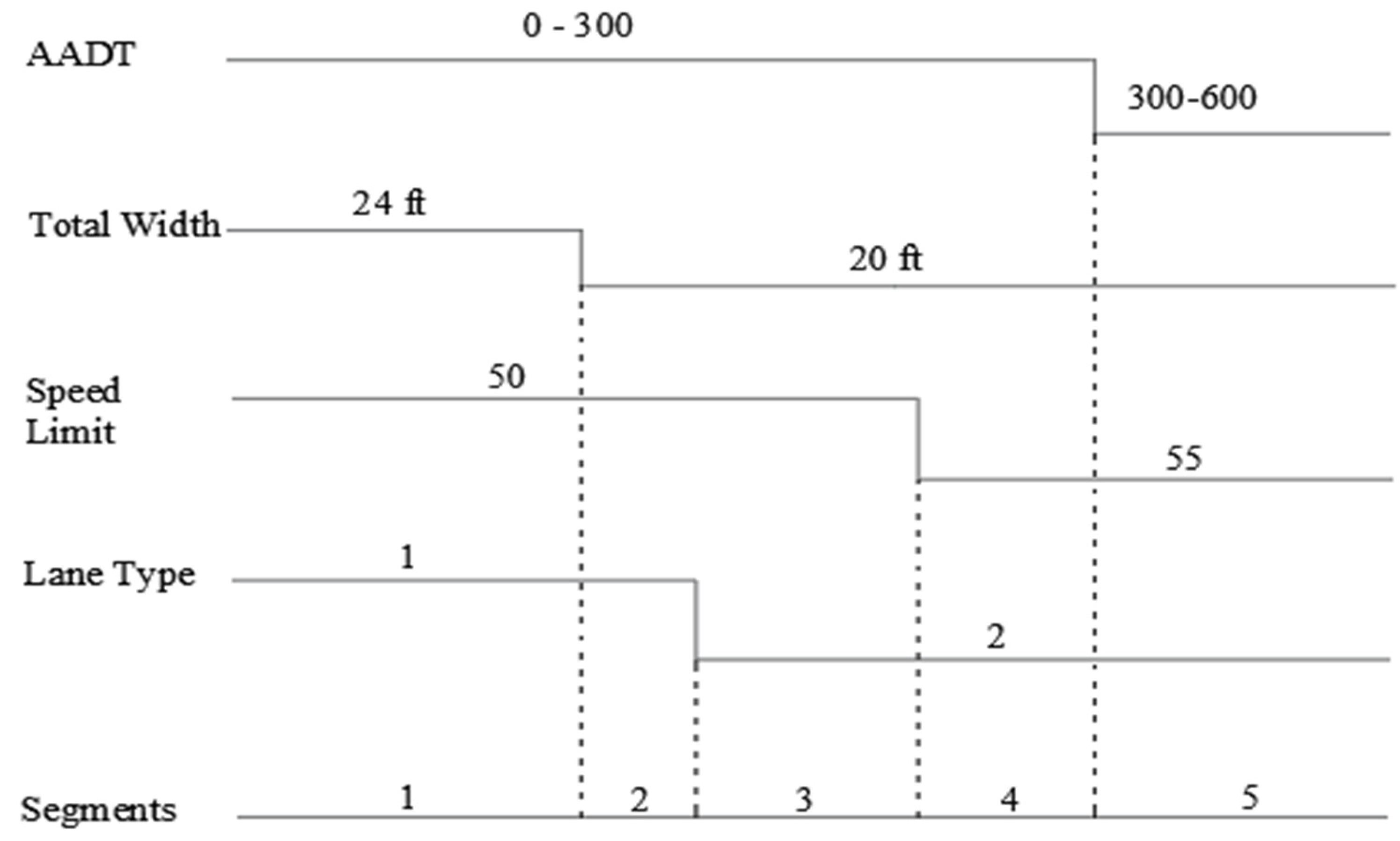
As mentioned earlier, the data were collected using 0.05-mile increments. Afterward, the total sample was compiled into homogeneous segments concerning the variables included in the scoring scheme, such as annual average daily traffic (AADT), speed limit, lane plus shoulder (total) width, side slope, and lane type. Any change in one or more variables marked the end of a segment and the beginning of another segment. For example, let us consider the 1-mile stretch of a highway segment shown in Figure 2. This stretch can be divided into five segments based on variations in AADT, total lane and shoulder width, lane type, and speed limit. Figure 2 illustrates the segmentation process, also reported in the work of Ambros et al. [18].

Upon completing the segmentation, a total of 377 segments were compiled. These segments were assigned scores using the proposed methodology, and the expected number of crashes was calculated for respective segments using the Empirical Bayes method. Crash frequency data for the period 2011–2020 were compiled for roadway segments for three different analysis periods (2011–2020, 2016–2020, and 2018–2020). Then, the observed crash frequencies and the EB expected number of crashes were normalized by length to find crash density, which was the basis for ranking segments in the study sample.

7. Methodology

The objective of the evaluation of the proposed method is to examine the effectiveness of the proposed screening method in identifying sites in need of safety improvement. The approach that was used in evaluating the proposed network screening method is to compare site rankings using the proposed method with the respective rankings using crash history data. Furthermore, rankings from the Empirical Bayes method were included in the analyses to see how the performance of the proposed method compares to that of the well-established Empirical Bayes technique. In the context of this study, “ranking” refers to the process of arranging roadway segments in accordance with their respective crash risk levels, with the intent of establishing a hierarchical order from segments exhibiting a high crash risk to those displaying a low crash risk. The Empirical Bayes method estimates the expected number of crashes at a site using the observed number of crashes and the predicted number of crashes found from the respective HSM safety performance function. Its main advantage is to alleviate the effect of randomness by not relying solely on crash history. The use of the Empirical Bayes method in this study is based on the fact that this technique has become the gold standard in performing quantitative safety analyses, with merits and effectiveness well established in the literature [19,20,21,22,23,24].

Three different analysis periods were used to check the consistency of the performance of the proposed method for network screening: three years, five years, and ten years. The use of three- and five-year study periods is consistent with the current practice in safety analyses, as found in many studies in the literature [7,23]. The rationale for using a ten-year analysis period is that, while crashes are rare events that tend to be randomly distributed over space and time, observing crash occurrence over an extended period of time is believed to largely alleviate the effect of randomness in crash data. Therefore, it was of interest to see how the analysis results may differ from the shorter study periods used in this study.

Initially, the proposed method was evaluated according to the rank correlation. Specifically, the Spearman rank correlation coefficient was calculated between the proposed method’s ranking and the ranking using observed crash data. Spearman’s rank correlation coefficient is a nonparametric or distribution-free rank statistical measure of the strength and the direction of the arbitrary monotonic association between two ranked variables or one ranked variable and one measurement variable [25]. Spearman’s rank correlation value varies from −1 to +1, where $\pm 1$ represents perfect correlation, and 0 means no correlation. The simple expression for Spearman coefficient “P” based on the difference between the two ranked variables is as shown in Equation (1):

$$P=1-\frac{6\Sigma d_i^2}{n^3-n}$$

(1)

where P = Spearman’s rank correlation coefficient; d_i = R(Xi) − R(Yi) is the difference between the two ranks of segment “i” by two compared methods; and n = number of observations.

In this study, the evaluation was carried out for five subsets of the total dataset (increasing 20 upper tails in the ranking list with each subset successively) and for the whole dataset, using the three different analysis periods. If the value is close to 1, the correlation is stronger, and the performance of the method is deemed more favorable.

Next, the proposed method is also analyzed according to the average difference between its ranking and the ranking of the observed crash data using the root mean square error [26] as in Equation (2):

$$RMSE=\sqrt{\frac{1}{n}\Sigma d_i^2}$$

(2)

where RMSE = root mean square error; d_i = R(Xi) − R(Yi) is the difference between the two ranks of segment i by two compared methods; n is the number of observations. The smaller the RMSE, the better the performance of the proposed method (i.e., less disparity between rankings).

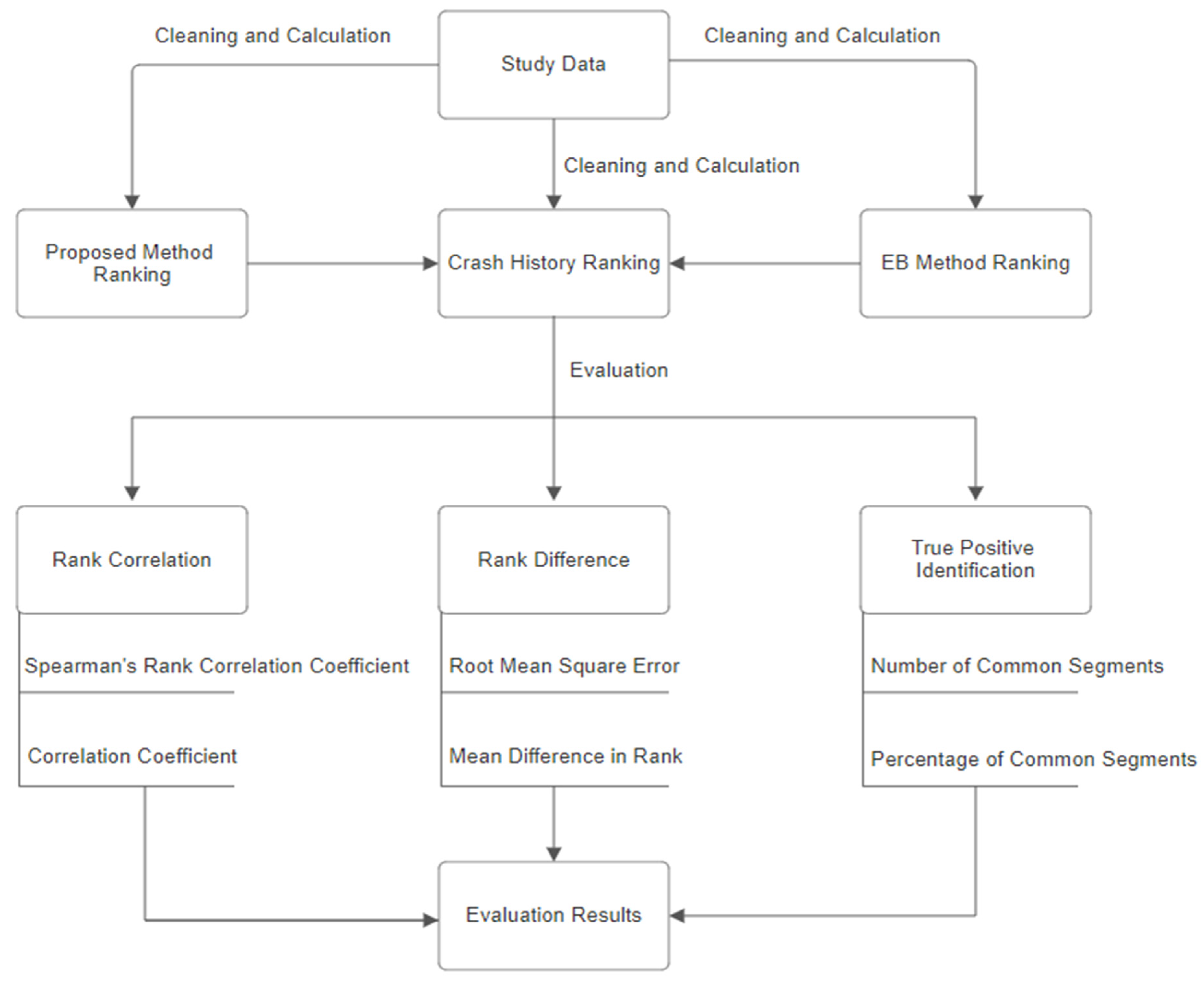
Finally, the number of sites identified as critical is estimated. This evaluation listed the number and percentage of common segments between two lists: the one compiled using ranks from the proposed method and the other using ranks from observed crash data. The higher the number and percentage of the common sites, the better the performance of the proposed method because this indicates a stronger match between the prediction of the proposed method and the real-world crash data. As discussed earlier, these analyses were also performed using the EB expected number of crashes that was used for comparison purposes. The data flowchart about the methodology for evaluating the network screening performance of the proposed method is shown in Figure 3.

8. Study Results

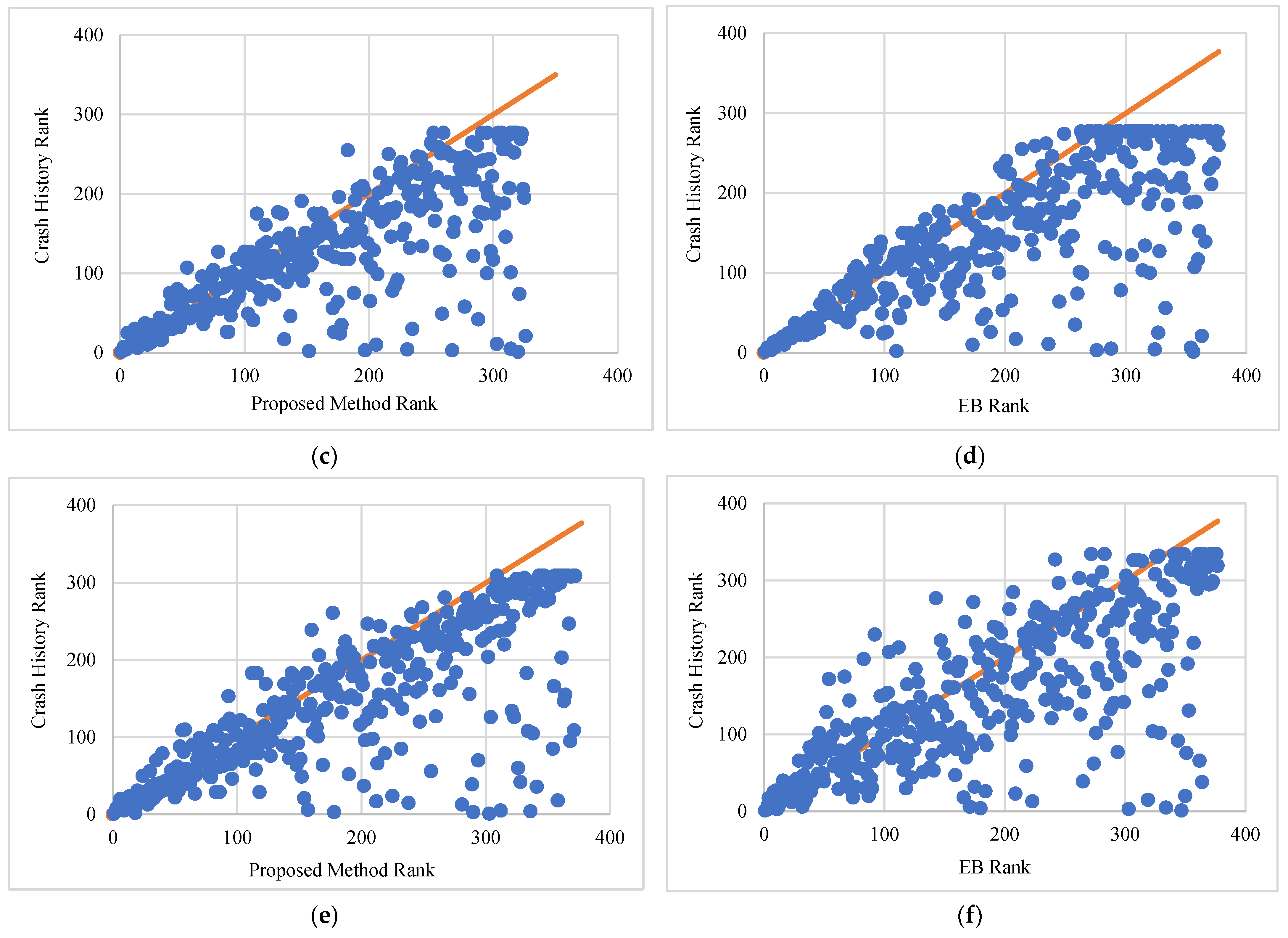
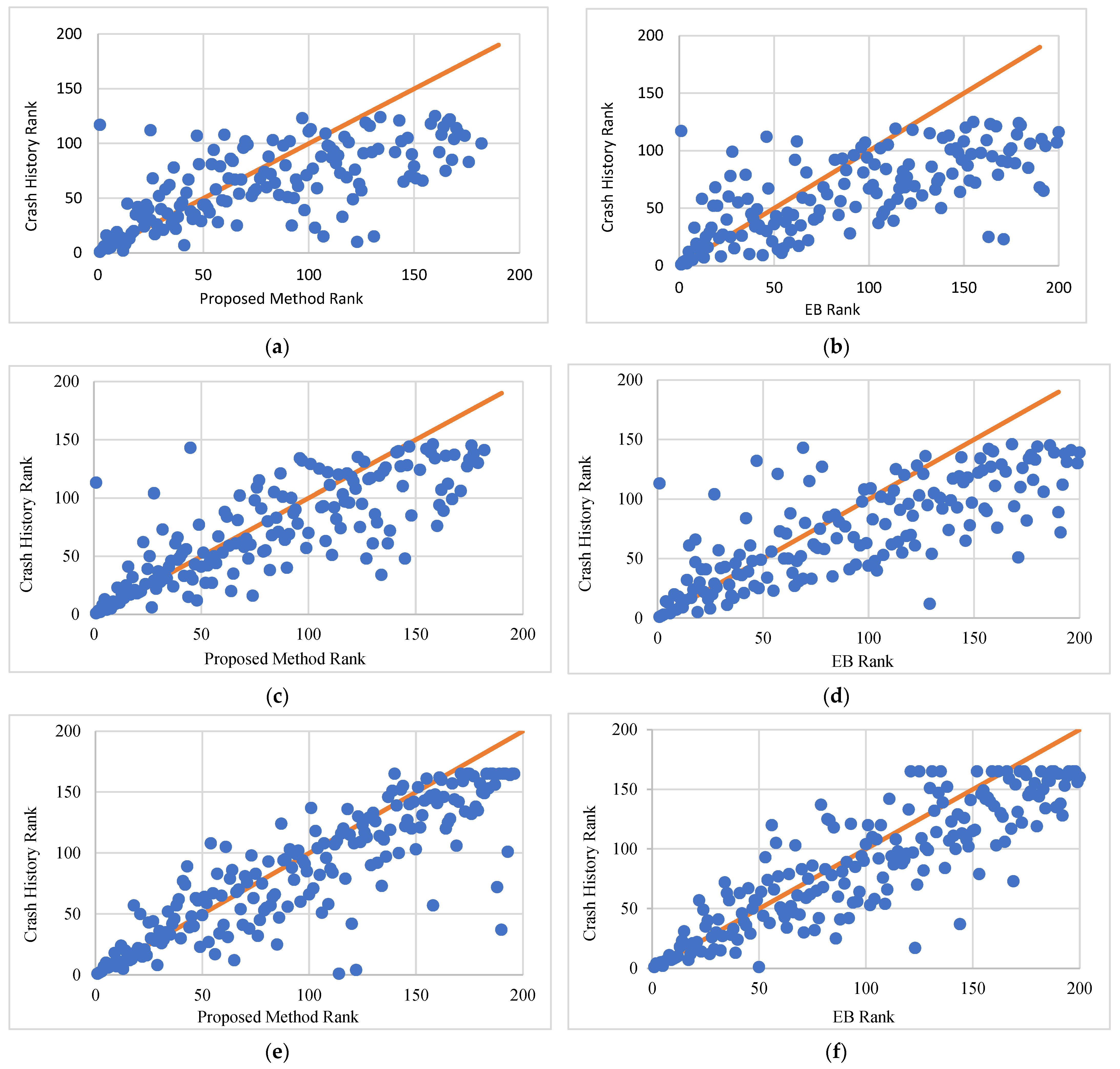
Figure 4 shows a scatterplot with site rankings using the proposed method and the EB method versus crash history for the three different analysis periods. A careful examination of all the scatterplots for the proposed method versus crash history (Figure 4a,c,e) reveals a few important observations. First, for most roadway segments, the two rankings correspond well to each other, as exhibited by the clustered observations around the diagonal line. This is particularly evident in sites that ranked high on the list (first seventy ranks for Figure 4a, and around a hundred ranks for Figure 4c,e). The figures also show a slight downward deviation of clustered observations below the diagonal line, which increases with the increase in rank. This is mostly the result of having two or more sites sharing the same rank using crash history (e.g., segments that had seen no crashes during the analysis period). This is confirmed by the fact that the total number of ranks using crash history is smaller than that using the proposed method. It is important to note that for observations that are scattered outside the diagonal cluster, the rank using crash history almost always resulted in sites being higher on the list (lower ranks) compared to the ranks using the proposed method (observations below the diagonal cluster). The tightness of the data points around the diagonal line in the scatterplot indicates a strong correlation between the two rankings, which is supported by a correlation coefficient of 0.821 for ten years of analysis. However, for the shorter study period of three years (Figure 4a), the data points are much more scattered compared to the longer analysis periods. This is due to the fact that for the shorter time period, more segments in the study sample had no crashes compared to those for longer analysis periods. A perfect correlation is visually represented as a straight diagonal line.

The EB method ranking was also compared with the ranking using the observed number of crashes, and the results are shown in Figure 4b,d,f for different analysis periods. In these figures, the proximity of data points to the line passing through the origin (diagonal line) indicates that it is somewhat scattered compared to that of the proposed method. This observation is confirmed by a slightly lower correlation coefficient (r = 0.781) between the two rankings for the ten-year study period. Also, for the three-year study period, the EB method exhibits somewhat similar observations to that of the proposed method. This is also the result of a large number of segments having no crashes. However, it is worth noting that the EB method shows better performance than the proposed method for the three-year period.

Further analyses were conducted to better understand the correlation between rankings using the proposed and the EB methods on one hand and crash history on the other hand, and the results are reported in

Table 2. Correlation coefficients for study sample for different analysis periods.

(# of Segments)	% of Sample Segments	Spearman’s Rank Correlation Coefficient		Correlation Coefficient
		Proposed Methodology	EB Method	Proposed Methodology	EB Method
Three-Year Analysis Period
Upper Tail (20)	5.31%	0.820	0.881	0.812	0.876
Upper tail (40)	10.61%	0.814	0.930	0.806	0.917
Upper Tail (60)	15.92%	0.834	0.921	0.828	0.902
Upper Tail (80)	21.22%	0.825	0.871	0.807	0.852
Upper Tail (100)	26.53%	0.835	0.837	0.813	0.824
Total (377)	100%	0.787	0.794	0.760	0.766
Five-Year Analysis Period
Upper Tail (20)	5.31%	0.801	0.792	0.784	0.787
Upper tail (40)	10.61%	0.876	0.830	0.841	0.776
Upper Tail (60)	15.92%	0.891	0.854	0.872	0.840
Upper Tail (80)	21.22%	0.884	0.814	0.875	0.792
Upper Tail (100)	26.53%	0.864	0.767	0.851	0.751
Total (377)	100%	0.821	0.801	0.811	0.786
Ten-Year Analysis Period
Upper Tail (20)	5.31%	0.952	0.832	0.949	0.834
Upper tail (40)	10.61%	0.966	0.930	0.969	0.935
Upper Tail (60)	15.92%	0.975	0.935	0.975	0.942
Upper Tail (80)	21.22%	0.951	0.915	0.957	0.934
Upper Tail (100)	26.53%	0.916	0.867	0.924	0.884
Total (377)	100%	0.821	0.794	0.854	0.824

. The table shows the values of Spearman’s rank correlation coefficient along with the correlation coefficient for the total study sample as well as for subsets of sample data using upper tail 20, 40, 60, 80, and 100 sites (top ranking sites on the list). Also, the results show that the consistency of the proposed method and crash history increases with the increase in the analysis period. This is both logical and expected, given that longer analysis periods are believed to alleviate the randomness in crash data.

The results clearly demonstrate that the proposed method consistently outperforms the Empirical Bayes method across upper tail segments and the total sample, as shown in Table 2 for the five-year and ten-year analysis periods. Higher correlation coefficients are observed for the proposed methodology in all segment categories, indicating a stronger association and better alignment with the observed crash data. For example, considering upper tail (20) segments for the ten-year period, which accounts for 5.31% of sample segments, the proposed methodology yields a Spearman’s rank correlation coefficient of 0.952 versus 0.832 for the Empirical Bayes method. Similarly, in the upper tail (100) segments, representing 26.53% of sample segments, the proposed methodology yields a correlation coefficient of 0.916 compared to 0.867 for the Empirical Bayes method. Using the total study sample, Spearman’s rank correlation coefficients for the proposed methodology (0.821) and the Empirical Bayes method (0.794) indicate the overall favorable performance of the two methods across all segments. The higher correlation coefficients signify a higher association between the rankings generated by the proposed method and the observed crash data.

However, the three-year study period shows that the EB method outperformed the proposed method in every upper tail group and the total sample when comparing the correlation coefficients and Spearman’s rank correlation coefficients.

Table 3. Mean difference in ranks and root mean square error for different analysis periods.

(# of Segments)	% of Sample Segments	Mean Difference in Rank		Root Mean Square Error
		Proposed Methodology	EB Method	Proposed Methodology	EB Method
Three-Year Analysis Period
Upper Tail (20)	5.31%	5.500	2.915	6.624	3.521
Upper tail (40)	10.61%	7.800	3.875	8.152	5.102
Upper Tail (60)	15.92%	11.750	5.617	13.245	7.655
Upper Tail (80)	21.22%	15.162	9.687	17.183	12.202
Upper Tail (100)	26.53%	18.520	13.31	20.224	18.323
Five-Year Analysis Period
Upper Tail (20)	5.31%	4.200	2.300	5.464	3.521
Upper tail (40)	10.61%	5.175	3.225	5.875	4.102
Upper Tail (60)	15.92%	5.933	4.667	7.229	5.655
Upper Tail (80)	21.22%	9.275	8.125	9.687	9.202
Upper Tail (100)	26.53%	12.190	11.970	13.187	12.323
Ten-Year Analysis Period
Upper Tail (20)	5.31%	5.250	7.300	6.124	9.124
Upper tail (40)	10.61%	7.475	11.000	8.412	12.142
Upper Tail (60)	15.92%	10.533	15.450	11.224	17.452
Upper Tail (80)	21.22%	12.037	19.237	13.450	21.230
Upper Tail (100)	26.53%	14.910	23.400	15.112	25.345

presents the rank root mean square error (RMSE) and mean rank difference for the proposed and the EB methods in reference to the observed crash history over the three different study periods. The rank RMSE and mean rank difference were estimated using upper tail segments for a total of 20, 40, 60, 80, and 100 segments. A quick examination of Table 3 indicates that, overall, as the percentage of upper tail segments increases, the mean difference between ranks and RMSE tends to increase for both methods. This trend indicates more discrepancies in rankings as the number of segments increases. For the three-year analysis period, the EB method consistently outperformed the proposed method with lower mean difference and RMSE values. The five-year analysis period still shows a better performance by the EB method compared with the proposed method; however, the discrepancies in mean difference and RMSE are not as significant and are relatively close, especially for upper tail groups 60, 80, and 100. Unexpectedly, the ten-year analysis period results showed a different trend than that of the shorter analysis periods. Specifically, the proposed method consistently outperformed the EB method for all upper tail groups using ten years of crash and traffic data. It is worth noting that the discrepancies in mean difference and RMSE for the ten-year analysis period are notable, generally in the order of 30 to 40 percent.

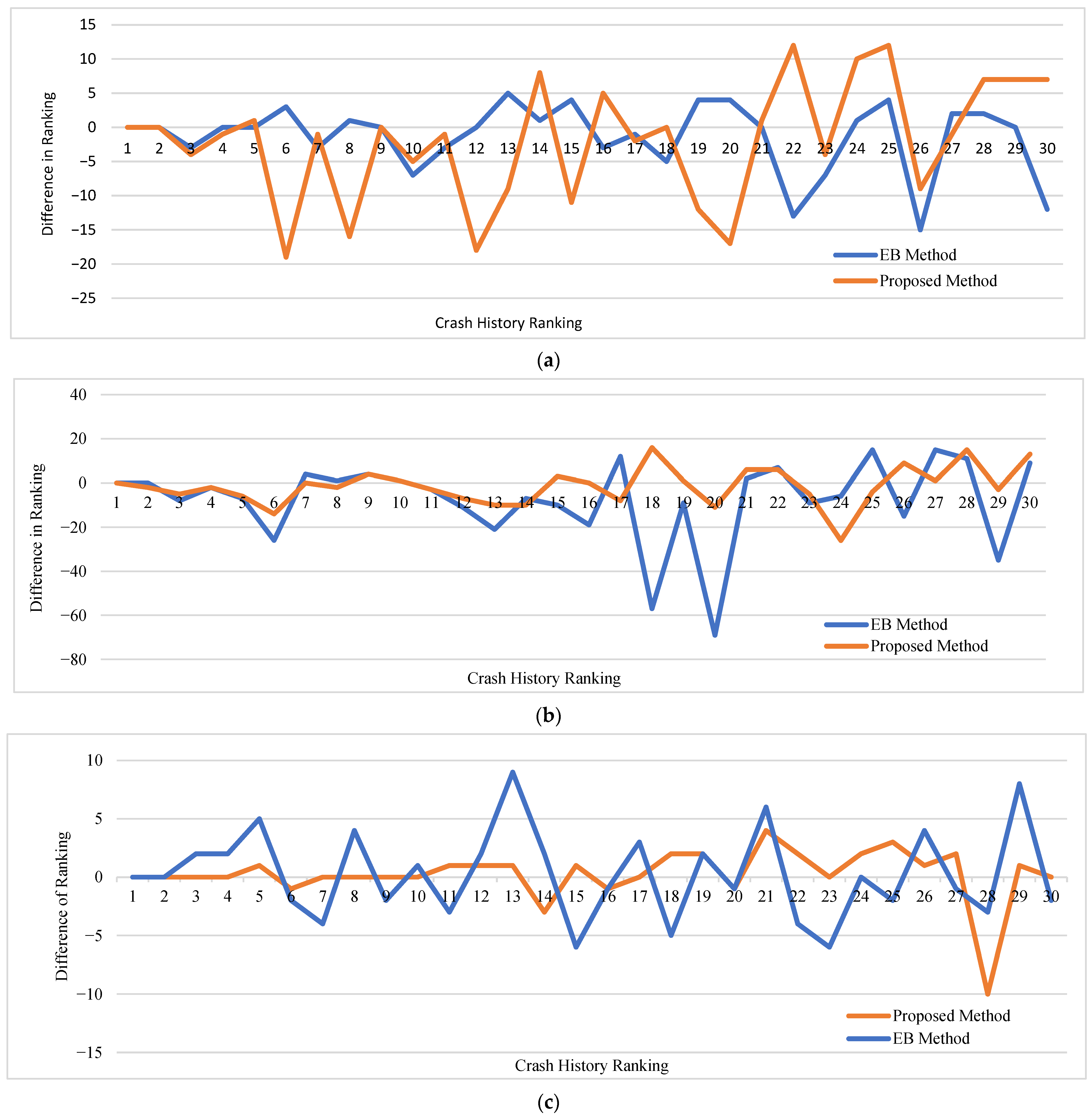
Figure 5 shows the difference in ranking between the crash history and that of the proposed and the EB methods for the first thirty highest-ranking segments in the study sample and for the three different analysis periods. The y-axis represents the difference between the ranks, while the x-axis represents the rank of the subject segment using the observed crash history.

This figure clearly shows a higher level of consistency between the proposed method ranks and the crash history ranks compared with that of the EB method for the 5-year and 10-year analysis periods. For the ten-year analysis period, the difference in ranks for the proposed method was between 0 and 2 in all observations except for ranks 21, 25, and 28, as shown in Figure 5c. However, when the analysis was performed using a three-year period, the EB method outperformed the proposed method with ranks showing higher consistency with the observed crash data.

Table 4. Number and percent of common segments with crash history for the proposed and the EB methods by various upper tail segment groups.

(# of Segments)	% of Sample Segments	# of Common Segments		% of Common Segments
		Proposed Method	EB Method	Proposed Method	EB Method
Three-Year Analysis Period
Upper Tail (20)	5.31%	13	19	65	95
Upper Tail (40)	10.61%	38	36	95	90
Upper Tail (60)	15.92%	54	53	90	88.33
Upper Tail (80)	21.22%	70	67	87.5	83.75
Upper Tail (100)	26.53%	88	85	88	85
Five-Year Analysis Period
Upper Tail (20)	5.31%	13	18	65	90
Upper Tail (40)	10.61%	39	36	97.5	90
Upper Tail (60)	15.92%	60	53	100	88.33
Upper Tail (80)	21.22%	80	67	100	83.75
Upper Tail (100)	26.53%	100	85	100	85
Ten-Year Analysis Period
Upper Tail (20)	5.31%	14	18	70	90
Upper Tail (40)	10.61%	39	38	97.5	95
Upper Tail (60)	15.92%	60	56	100	93.33
Upper Tail (80)	21.22%	80	74	100	92.5
Upper Tail (100)	26.53%	100	92	100	92

presents the results of identifying true positive segments with a crash history for the proposed method and the EB method across different upper tail segment groups and analysis periods. The results are presented in terms of the number of common segments and the percentage of common segments identified by both methods.

For every analysis period, the proposed method identified more true positive sites in all upper tail segments except for the upper tail (20), where the data show less favorable performance of the proposed method. Specifically, in considering five-year and ten-year study periods, the proposed method identified 100% of the segments as identified by the crash history ranking for upper tails 60 or greater. For the upper tail (40), the proposed method identified 97.5% of true positive segments under both study periods. While the percent common segments for the EB method was 80% or higher for all upper tail segments, the proposed method consistently outperformed the EB method for being more consistent with the crash history rankings for all upper tail segment groups except for the upper tail (20).

8.1. Traffic Volume Investigation

As discussed earlier, the development of the proposed method was largely based on the HSM safety performance functions and crash modification factors for rural two-lane highway segments and intersections. Therefore, the proposed method should be applicable to rural two-lane highways regardless of traffic volume. However, as the method was specifically proposed for use on low-volume roads, it is deemed valuable to evaluate the effectiveness of the proposed method for lower as well as higher traffic volumes. The results of this investigation are presented in this section.

8.1.1. Low-Volume Roads Analysis

In this study, low-volume roads are defined as rural two-lane highways with Average Annual Daily Traffic (AADT) equal to or less than 1000 vehicles per day. This is consistent with a few other studies that used the same definition in the literature [27,28]. Approximately a total of 850 miles representing 200 segments of state-owned and operated low-volume roads were used in this analysis.

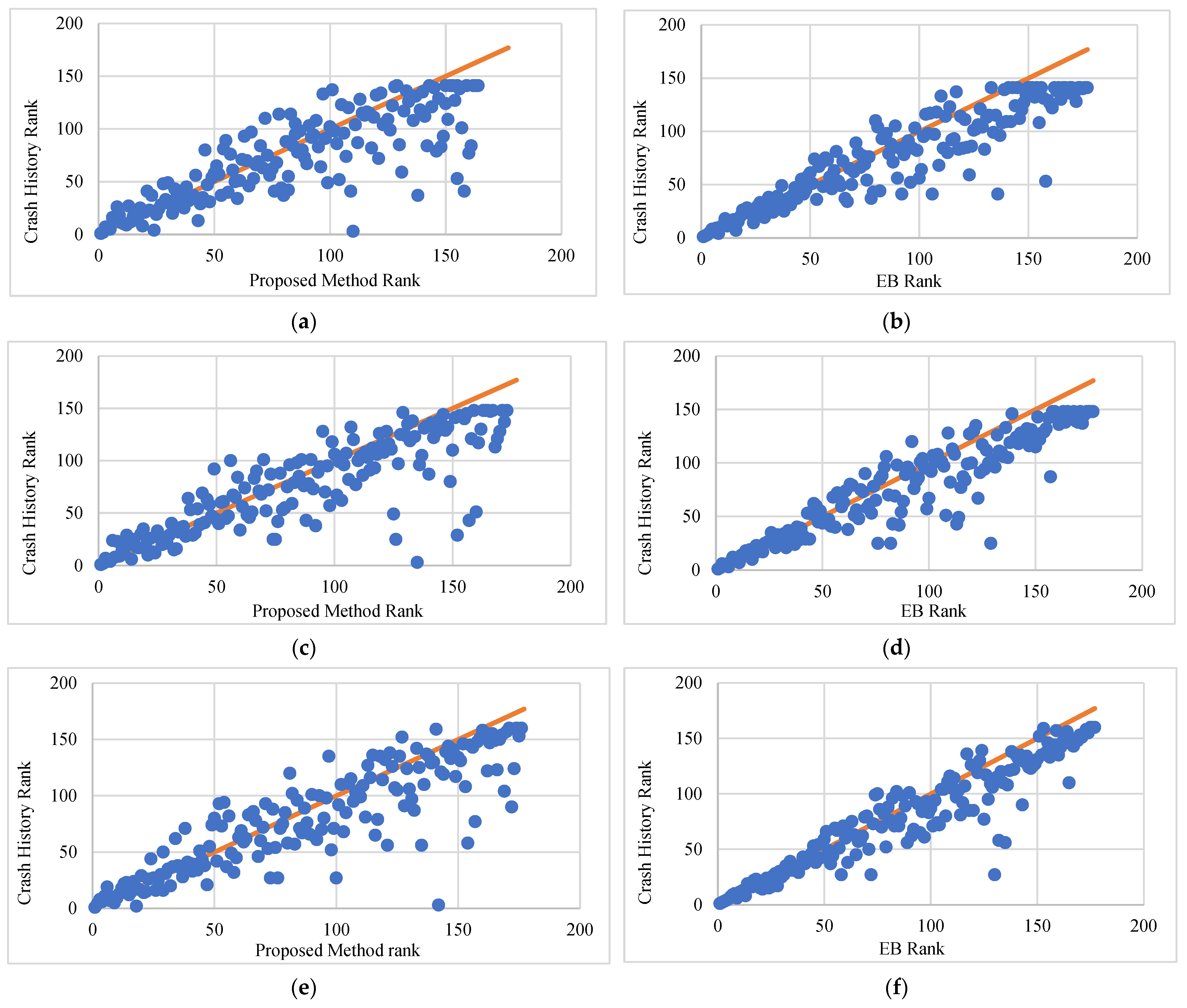
Figure 6 shows scatterplots with rankings by the proposed method and the EB method versus the observed crash history for different analysis periods. As shown in Figure 6a,c,e for the proposed method and observed crash history, the consistency between the two rankings increases steadily with the increase in the analysis period. This is evident in the density of data points clustered around the diagonal line (the correlation coefficient is 0.742, 0.817, and 0.869 for three, five, and ten years, respectively). The general pattern shown here is consistent with that shown in Figure 4 for the whole dataset. This is due to the fact that a larger number of segments do not have crashes when shorter analysis periods are used. This is also evident in the total number of ranks for different analysis periods.

Figure 6b,d,f, which compare rankings by the EB method and observed crash data, show similar patterns with slightly more scattered around the diagonal line. Specifically, the coefficients of correlation are only 0.647, 0.734, and 0.854 for the three analysis periods, which indicate good yet less consistent relationships between the two rankings compared to those of the proposed method. The increase in correlation coefficients for longer analysis periods is similar to the case of the proposed method.

Table 5. Ranking consistency metrics for the proposed and the EB method—low-volume roads.

Metrics	Proposed Method	Empirical Bayes Method
Three-Year Analysis Period
Spearman’s Rank Correlation Coefficient	0.760	0.617
Correlation Coefficient	0.742	0.637
Average Difference in Ranking	28.415	38.912
Root Mean Square Error	29.753	40.201
Five-Year Analysis Period
Spearman’s Rank Correlation Coefficient	0.842	0.724
Correlation Coefficient	0.817	0.734
Average Difference in Ranking	21.415	31.645
Root Mean Square Error	23.753	36.311
Ten-Year Analysis Period
Spearman’s Rank Correlation Coefficient	0.853	0.847
Correlation Coefficient	0.868	0.857
Average Difference in Ranking	19.415	22.885
Root Mean Square Error	21.753	25.311

provides the Spearman’s rank correlation coefficient, the correlation coefficient, the average rank difference, and the rank RMSE for the proposed and the EB methods. As shown clearly in this table, the proposed method consistently outperforms the EB method in every metric for all low-volume road segments (200 segments) and for each study period. The average difference in rankings and root mean square errors decreases with the increase in the analysis period, whereas the correlation coefficients increase with the increase in the analysis period for both methods. This was discussed earlier in discussing results for the whole dataset.

Table 6. Number and percent of common segments with crash history for the proposed and the EB methods for various upper tail segment groups—low-volume roads.

(# of Segments)	% of Sample Segments	# of Common Segments		% of Common Segments
		Proposed Method	EB Method	Proposed Method	EB Method
Three-Year Analysis Period
Upper Tail (10)	5.00%	6	6	60	60
Upper Tail (20)	10.00%	15	12	75	60
Upper Tail (30)	15.00%	19	25	63.33	60
Upper Tail (40)	20.00%	28	24	70	60
Upper Tail (50)	25.00%	39	33	78	66
Five-Year Analysis Period
Upper Tail (10)	5.00%	8	6	80	60
Upper Tail (20)	10.00%	15	14	75	70
Upper Tail (30)	15.00%	23	21	76.67	70
Upper Tail (40)	20.00%	29	29	72.5	72.5
Upper Tail (50)	25.00%	40	38	80	76
Ten-Year Analysis Period
Upper Tail (10)	5.00%	7	7	70	70
Upper Tail (20)	10.00%	15	16	75	80
Upper Tail (30)	15.00%	26	25	86.67	83.33
Upper Tail (40)	20.00%	33	32	82.5	80
Upper Tail (50)	25.00%	44	39	88	78

shows the number and percentage of common segments for various upper tail segment groups for the proposed and the EB methods separately. Overall, the results for the two methods are comparable, with slightly better performance exhibited by the proposed method for the three analysis periods.

8.1.2. Higher Volume Roads

In this analysis, higher volume roads represent the rest of the dataset, i.e., roads with AADT greater than 1000 vehicles per day. Around 645 miles of two-lane roadways were extracted from the dataset, accounting for 177 total segments for the analysis.

The consistency of rankings between the proposed method, the EB method, and the observed crash history is shown in Figure 7. While the data points in Figure 7a,c,e show a relatively good relationship between the rankings of crash history and the proposed method, it is not as strong as that for the crash history and EB method shown in Figure 7b,d,f. This is contradictory to the trend shown in Figure 6 for low-volume roads.

Table 7. Ranking consistency metrics for proposed and the EB methods—higher volume roads.

Metrics	Proposed Method	Empirical Bayes Method
Three-Year Analysis Period
Spearman’s Rank Correlation Coefficient	0.844	0.889
Correlation Coefficient	0.840	0.917
Average Difference in Rank	19.186	17.446
Root Mean Square Error	22.745	20.355
Five-Year Analysis Period
Spearman’s Rank Correlation Coefficient	0.841	0.903
Correlation Coefficient	0.848	0.927
Average Difference in Rank	18.723	16.969
Root Mean Square Error	21.745	18.169
Ten-Year Analysis Period
Spearman’s Rank Correlation Coefficient	0.866	0.924
Correlation Coefficient	0.871	0.941
Average Difference in Rank	17.875	13.536
Root Mean Square Error	19.745	15.355

provides Spearman’s rank correlation coefficient, correlation coefficient, average rank difference, and rank RMSE for the proposed and the EB methods using rankings by crash history as a reference for three analysis periods. This table clearly shows that for the higher-volume roads, the EB method rankings are more consistent with those of the observed crash history than the rankings of the proposed method. This is contrary to the respective trend discussed in the low-volume road analysis. However, it should be mentioned that the correlation coefficients still suggest a relatively strong relationship between the proposed method ranks and those of the observed crash history.

The number and percentage of common segments for the proposed and the EB methods with those of the observed crash history for the three different analysis periods are provided in

Table 8. Number and percent of common segments with crash history for the proposed and the EB methods for various upper tail segment groups -higher volume roads.

(# of Segments)	% of Sample Segments	# of Common Segments		% of Common Segments
		Proposed Method	EB Method	Proposed Method	EB Method
Three-Year Analysis Period
Upper Tail (10)	5.60%	5	9	50	90
Upper Tail (20)	11.20%	15	18	75	90
Upper Tail (30)	16.90%	25	27	83.33	90
Upper Tail (40)	22.60%	33	36	82.5	90
Upper Tail (50)	28.40%	42	44	84	88
Five-Year Analysis Period
Upper Tail (10)	5.60%	7	8	70	80
Upper Tail (20)	11.20%	13	18	65	90
Upper Tail (30)	16.90%	26	26	86.67	86.67
Upper Tail (40)	22.60%	36	37	90	92.5
Upper Tail (50)	28.40%	42	45	84	90
Ten-Year Analysis Period
Upper Tail (10)	5.60%	8	9	80	90
Upper Tail (20)	11.20%	15	16	75	80
Upper Tail (30)	16.90%	26	29	86.67	96.67
Upper Tail (40)	22.60%	34	38	85	95
Upper Tail (50)	28.40%	44	46	88	92

. As shown in this table, the EB method outperforms the proposed method in all upper tail segment groups. While this may initially seem unexpected, it can easily be explained with a proper understanding of the EB method formulation. Specifically, the contribution of crash history in the EB expected number of crashes increases with traffic volume, and thus the correlation between crash history and the EB expected number of crashes. This explains why results for the low-volume roads and higher-volume roads are somewhat different.

9. Summary and Conclusions

Road safety management programs constitute a fundamental element in advancing sustainable mobility. Proper identification of safety improvement sites via network screening is critical for the success of these programs. This study aimed to evaluate the performance of a new, proposed, and simplistic network screening method for identifying candidate sites for safety improvements on rural two-lane roads. The proposed method is largely based on the HSM safety performance functions and crash modification factors and was originally proposed for use on low-volume roads. Roadway geometry, roadside characteristics, traffic, and crash data were acquired for the 1495-mile study sample using Oregon DOT online databases and archived video logs. In this study, three different analysis periods (three years, five years, and ten years) were used in the evaluation, with the Empirical Bayes method also analyzed for comparison purposes.

Study results showed an overall strong performance of the proposed method in identifying candidate sites for safety improvements. Given the simplicity and limited data requirements of the proposed method, it can provide a viable option for network screening in cases where the use of the well-established EB method is deemed impractical for lack of accessible data or technical expertise (e.g., roads owned and operated by local agencies such as counties, townships, and tribal governments).

The proposed method outperformed the well-established EB method when the whole study sample was used in the analysis. However, when the study sample was split into two datasets based on traffic volume, the proposed method outperformed the EB method for low-volume roads, while the EB method was found more effective for higher-volume roads. This can be explained by the fact that the contribution of crash history into the EB expected number of crashes increases with traffic volume, thus the more consistency between the two. Therefore, the use of the proposed method, while overall effective, can be particularly valuable for use on low-volume roads for its better performance and ease of implementation, particularly by local agencies.

The proposed screening method was originally developed for the application on low-volume roads. Nevertheless, the performance has been assessed for low and higher traffic volumes, extending up to 4000 ADT (Annual Daily Traffic). It is worth noting that for exceptionally high traffic volumes, the effectiveness of the proposed method may be limited.

The evaluation was conducted using data exclusively from the state of Oregon. However, for a comprehensive assessment, the authors recommend using data from other states and regions.