Article

Vegetation Type Mapping in Southern Patagonia and Its Relationship with Ecosystem Services, Soil Carbon Stock, and Biodiversity

by
Pablo L. Peri
1,2,*,
Juan Gaitán
3,
Boris Díaz
1,
Leandro Almonacid
1,
Cristian Morales
1,
Francisco Ferrer
2,
Romina Lasagno
1,
Julián Rodríguez-Souilla
4 and
Guillermo Martínez Pastur
4
1
Instituto Nacional de Tecnología Agropecuaria (INTA), Río Gallegos 9400, Argentina
2
Natural Resources Department, Universidad Nacional de la Patagonia Austral (UNPA)—CONICET, Río Gallegos 9400, Argentina
3
Consejo Nacional de Investigaciones Científicas y Técnicas (CONICET), Universidad Nacional de Luján, Luján 6700, Argentina
4
Laboratorio de Recursos Agroforestales, Centro Austral de Investigaciones Científicas (CADIC CONICET), Ushuaia 9410, Argentina
*
Author to whom correspondence should be addressed.
Sustainability 2024, 16(5), 2025; https://doi.org/10.3390/su16052025
Submission received: 5 January 2024 / Revised: 15 February 2024 / Accepted: 27 February 2024 / Published: 29 February 2024

Abstract

:
Vegetation Type (VT) mapping using Optical Earth observation data is essential for the management and conservation of natural resources, as well as for the evaluation of the supply of provisioning ecosystem services (ESs), the maintenance of ecosystem functions, and the conservation of biodiversity in anthropized environments. The main objective of the present work was to determine the spatial patterns of VTs related to climatic, topographic, and spectral variables across Santa Cruz province (Southern Patagonia, Argentina) in order to improve our understanding of land use cover at the regional scale. Also, we examined the spatial relationship between VTs and potential biodiversity (PB), ESs, and soil organic content (SOC) across our study region. We sampled 59,285 sites sorted into 19 major categories of land cover with a reliable discrimination level from field measurements. We selected 31 potential predictive environmental dataset covariates, which represent key factors for the spatial distribution of land cover such as climate (four), topography (three), and spectral (24) factors. All covariate maps were generated or uploaded to the Google Earth Engine cloud-based computing platform for subsequent modeling. A total of 270,292 sampling points were used for validation of the obtained classification map. The main land cover area estimates extracted from the map at the regional level identified about 142,085 km2 of grasslands (representing 58.1% of the total area), 38,355 km2 of Mata Negra Matorral thicket (15.7%), and about 25,189 km2 of bare soil (10.3%). From validation, the Overall Accuracy and the Kappa coefficient values for the classification map were 90.40% and 0.87, respectively. Pure and mixed forests presented the maximum SOC (11.3–11.8 kg m−2), followed by peatlands (10.6 kg m−2) and deciduous Nothofagus forests (10.5 kg m−2). The potential biodiversity was higher in some shrublands (64.1% in Mata Verde shrublands and 63.7% in mixed shrublands) and was comparable to those values found for open deciduous forests (Nothofagus antarctica forest with 60.4%). The provision of ESs presented maximum values at pure evergreen forests (56.7%) and minimum values at some shrubland types (Mata Negra Matorral thicket and mixed shrubland) and steppe grasslands (29.7–30.9%). This study has provided an accurate land cover and VT map that provides crucial information for ecological studies, biodiversity conservation, vegetation management and restoration, and regional strategic decision-making.

1. Introduction

Planning and land management institutions need comprehensive information on the types of land-use cover to provide the basis for understanding the status, trends, and pressures of human activity on natural resources, carbon cycles, and biodiversity [1,2]. From this, Vegetation Type (VT) mapping using Optical Earth observation (EO) data is essential for the management and conservation of natural resources, as well as for the evaluation of the supply of provisioning ecosystem services (ESs), the maintenance of ecosystem functions, and the conservation of biodiversity in anthropized environments [3,4,5]. VTs are defined as distinctive lands that produce different types of vegetation with contrasting net primary production (NPP) and land uses [6,7]. For instance, climate determines two contrasting regions in Sothern Patagonia: a western narrow strip of land (100 km wide) with a humid climate and precipitation of up to 1200 mm/year being forest, the predominant vegetation type used for logging and silvopastoral systems. In the rest of the territory, where the westerly dry winds define the steppe ecosystem with precipitation of less than 300 mm/year, the main activity is extensive sheep (mostly of Merino and Corriedale breeds) production reared for meat and wool on natural grasslands [8,9,10]. Moreover, VTs describe the potential plant species growing at a site with similar ecological responses to natural drivers and management practices, and also, VT descriptions provide information to farmers about which changes can be expected in response to grazing management in productivity, carbon stocks, or potential climate change events [11,12,13].
VTs usually represent complex spatial structures within a heterogeneous landscape. Vegetation heterogeneity has been studied mainly in northeastern Patagonia at microsite, patch, and patch mosaic scales and at regional scales, where biotic and abiotic factors determine their spatial distribution [14,15]. In contrast, studies of VTs at the landscape or regional scale in Southern Patagonia are lacking. The creation of accurate VT maps in heterogeneous landscapes is usually based on the classification of raw satellite imagery. However, since the spatial and temporal resolution of satellite images is often insufficient to classify small VT structures in the landscape, heterogeneous plant covers pose a challenge for spectral classification methods that use EO images of a single datum [16]. In addition, multi-temporal Landsat images can improve the accuracy of VT classification and plant cover mapping in grasslands as they show different phases of vegetation phenology over single growing seasons [17]. Also, the use of multi-temporal Landsat data may compensate for poor quality observations (clouds, shadows) and better capture the phenological information of VTs in classification [18].
The Google Earth Engine (GEE) stores satellite imagery in a public data archive that includes historical Earth images, enabling researchers to select and process large volumes of data [18]. The open access to GEE allows users to analyze all available remote sensing images with a web-based IDE code editor without downloading these images to a local server [18]. In addition, the cloud-based platform provides basic computational capabilities for vector and raster data. Its high computing power enables land mapping approaches at regional, national, and global scales. GEE has been used extensively in numerous data processing applications and environmental studies, such as studies of forest degradation, vegetation succession in grassland ecosystems, and farmland classification [19,20,21].
Furthermore, VTs provide different ecosystem services (ESs), which refer to the different goods and benefits that society obtains directly or indirectly from natural ecosystems that contribute to human well-being [22]. ESs include (i) provisioning services (e.g., food, timber, and medicines), (ii) regulating services (e.g., water regulation, air quality maintenance, pollination, and climate control), (iii) cultural services (e.g., recreation opportunities, sense of place, and opportunities for education and identity), and (iv) supporting services (e.g., soil formation, primary productivity, biogeochemistry, nutrient cycling, and provisioning of habitat) [23]. Soil organic carbon (SOC) plays an important role in ecosystem service delivery, including biodiversity support, soil aggregation, soil erosion control, the capacity of the land to sustain plant and animal productivity, and water retention capacity [24]. Biodiversity conservation at different levels (e.g., genes, species, and ecosystems) supports the ecological processes and functions that sustain ESs and human well-being [25].
The objective of the present work was to determine the spatial patterns of VTs related to climatic, topographic, and spectral variables across Santa Cruz province in order to improve our understanding of land use cover at the regional scale. Also, we examined spatial relationships among VTs and potential plant biodiversity, ES, and SOC across our study region.

2. Materials and Methods

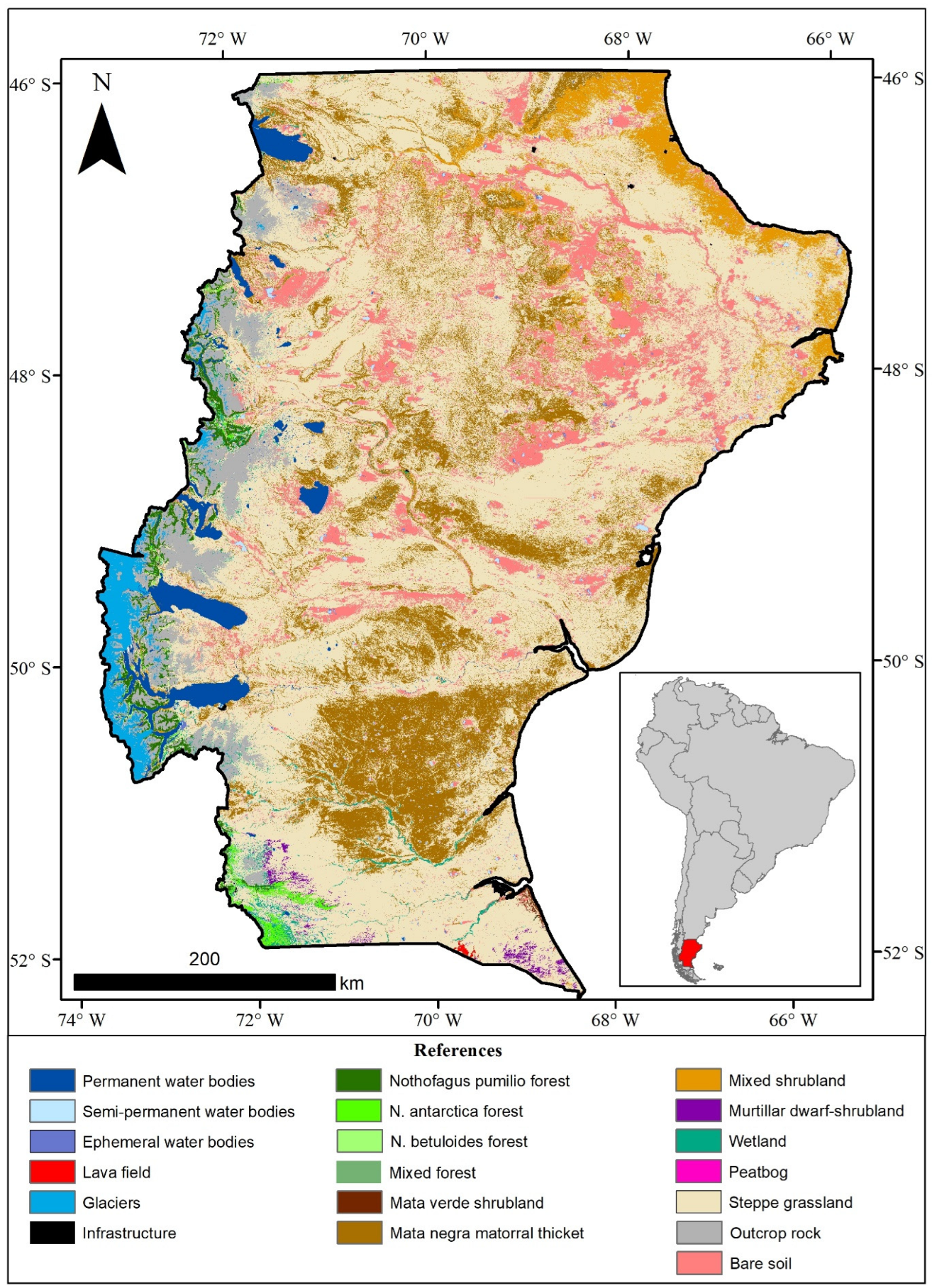
2.1. Characterization of the Study Area and Land Use Cover Classes

The study area corresponded to the whole Santa Cruz province, which has an area of 244,458 km2 and extends from latitudes 46° to 52°30′ SL. In the region, precipitation decreases from 800–1000 mm to 200 mm/year from west to east over the Andes Mountains, which act as an orographic barrier to humid winds from the west. This determines the aridity index (average annual ratio of precipitation to potential evapotranspiration), which varies between 0.45 and 0.11 in most of the region (85% of the total area corresponding to drylands), whereas aridity index values of >0.65 are found in native forest growing in the west, with a significant water deficit in the soil in the summer. The average annual temperatures are between 5.5 and 8.0 °C. The winds mainly come from the west and often reach wind speeds of over 80 km/h in the spring and summer. Local edaphic and topographic differences in combination with a considerable precipitation gradient have a significant influence on forage production in the meadows.
In this work, we sampled 59,285 sites in Santa Cruz province sorted into 19 major categories of land cover with a reliable discrimination level from field measurements: permanent water bodies, semi-permanent water bodies, ephemeral water bodies, lava fields, outcrop rock, bare soil, glacier, infrastructure, steppe grasslands, Mata Negra Matorral thicket, Mata Verde shrubland, mixed shrubland, Murtillar dwarf-shrubland, wetlands, peatbogs, Nothofagus antarctica forest, N. pumilio forest, N. betuloides forest, and mixed forest.
The cover of water bodies was evaluated considering that shallow waters usually present a strong dynamic of expansion and contraction between the wet and dry seasons of the year. Due to this, we obtained the frequency with which water was present from global maps of the location and temporal distribution of surface water from 1984 to 2021 [26] to discriminate: permanent water, when a pixel presented a >90% probability of presenting water; semi-permanent water bodies, when its probability was between 20 and 90%; and ephemeral water bodies, when it was <20% mainly concentrated in the late winter or early spring.
The lava field cover consists of basaltic formations without vegetation on the surface that originated from volcanic–tectonic between the Pliocene (3.8 million years ago) and the Lower Pleistocene (1 million years ago) [27]. Although the name “lavic field” usually refers to the Pali Aike lava field, located in the southeastern portion of the province, this cover map also includes other contemporary basaltic manifestations that are not or barely vegetated at present. Outcrop rock cover corresponds to any natural or anthropized areas (quarrying areas) devoid of soil. In general, it represents high mountainous areas. The bare soil category represents a soil surface devoid of any plant material or with a vegetation cover of less than 10% originating from natural (alpine sites) or anthropogenic processes and origins such as wind erosion, water erosion, fires, dunes, dry lagoons beds, deflation basins, road construction, and oil platforms. To define glacier cover, a mask was applied using the geoinformation database from the First National Glacier Inventory of the Argentine for the period 2004–2016 [28]. The infrastructure cover that included urbanized, peri-urban, and rural constructions was obtained and masked using polygons reported by the IGN [29].
The VT of steppe grasslands includes two different physiognomies: grass–shrub steppe in the center and north of the region and grass steppes in the south. The grass steppe is dominated by grasses and sedges (Bromus, Carex, Festuca, Hordeum, Jarava, Poa, Rytidosperma virescens, and Trisetum) with dwarf shrubs and herbs such as Nardophyllum, Perezia, Azorella, and Nassauvia admixed. The grass–shrub steppe is dominated by Jarava, Agrostis, Festuca, Hordeum, Trisetum, and shrubs (Berberis, Adesmia, Chuquiraga, Mulinum, Mulguraea tridens, Schinus, and Senecio). The VT category of shrubland, defined as an area where vegetation is dominated by woody plants (>40%) generally less than 3 m in height, has been divided into three distinctive categories. The Mata Negra Matorral thicket is dominated by the evergreen shrub M. tridens, which is sclerophyllous (“hard-leaved”) and grows continuously and intermixed with xeric steppe vegetation, creating spatial heterogeneity in the landscape as a result of vegetation patches. The Mata Verde shrubland is dominated by Lepidophyllum cupressiforme, a woody endemic species of 0.50 m in height, which develops in saline and sandy depressions on seashores and riverbeds, jointly with halophytic steppe species [30]. The mixed shrubland is dominated mainly by tall shrubs, such as Colliguaja integerrima, Chuquiraga, Anartrophyllum rigidum, Lycium, and Mulinum, and is dominated by grass-rich undergrowth including Bromus, Hordeum, Jarava, and Poa. The Murtillar dwarf-shrubland vegetation class is dominated by Empetrum rubrum, and dwarf-shrub heaths are associated with acidic, poor nutrient soils of coarse texture and disturbances such as overgrazing and fires [31]. Wetlands of Cyperaceae, Juncaceae, and Gramineae, locally known as “mallines”, are developed in association with conditions of the landscape where an unusual amount of water is available for plants [32]. Mallines provide the most productive soils for livestock production, and these are mainly located in floodplains, glacial plains, and hydro-eolian basins. Peatbogs are distinctive Sphagnum wetlands of Patagonia that represent a valuable natural resource that provides peat, moss fibers, and water, as well as the natural products that grow on its surface [33,34]. For this work, we used permanent plots across Santa Cruz province from the PEBANPA (Parcelas de Ecología y Biodiversidad de Ambientes Naturales en Patagonia Austral—Biodiversity and Ecological Long-term Plots in Southern Patagonia) network located in all VTs.
Nothofagus forests are mainly associated with the mountain areas, occupying a narrow strip in the west. Four main forest types occur in the region of Santa Cruz province [35,36]. The southern beech, ñire (Nothofagus antarctica), one of the main deciduous native species in this region, grows in pure stands and occurs naturally in different habitats such as poorly drained sites at low elevations, exposed windy areas with shallow soils, depressions under cold air influence, or drier eastern sites near the Patagonian steppe [37]. Pure deciduous Nothofagus pumilio (lenga) forests occur in the subalpine zone and commonly form the upper tree limit in mountain environments [36]. Pure evergreen Nothofagus betuloides (guindo) forests generally grow along the coast of the lake, where temperatures are milder and rainfall is higher. The mixed forests are dominated by evergreen N. betuloides and other Nothofagus species, as well as other secondary tree species (Drimys winteri, Embothrium coccineum, and Maytenus boaria) that grow in wet areas associated with mountain environments, mainly located in protected natural areas. To define the native forest cover, a mask was applied using the geoinformation database from forestry inventories across Santa Cruz province [35,36].

2.2. Environmental Predictors for the Land Cover Map

We selected 35 potential predictive environmental dataset covariates, which represent key factors for the spatial distribution of land cover such as climate (4), topography (3), and spectral (28) factors. All covariate maps were generated or uploaded to the Google Earth Engine cloud-based computing platform for subsequent modeling [38]. The original covariates’ spatial resolution was adjusted to a common resolution of 30 m.
We included climatic variables (more specifically, precipitation and temperature) because the distribution of VTs is closely coupled with corresponding climate types, and also because climate affects net primary productivity (NPP) [39]. Data on the mean (1970–2000) annual precipitation and monthly mean, minimum, and maximum temperature were obtained from the WorldClim global database. Derived from these monthly temperature and precipitation data, we used a group of 17 maps of bioclimatic variables [40].
Topography has the potential to control the spatial patterns of vegetation communities and cover and, therefore, models that take topographic variables into account can provide better estimates of VTs and land cover [41]. This is because topography, through its influence on gravity, solar insolation, and micro-climate, determines the water, solute, and sediment fluxes throughout the landscape. Altitude, slope, and aspect data derived from the ALOS World 3D at 30 m (AW3D30) digital elevation model (JAXA/ALOS/AW3D30/V3_2 Collection) were used [42].
For spectral variables, Landsat 8 satellite images of surface reflectance (Collection LANDSAT/LC08/C02/T1_L2) corresponding to the period 1 January 2017–21 December 2022 were used. Scenes with cloud cover greater than 30% were eliminated. For this, the QA_PIXEL band was used to filter those pixels with poor quality that were associated with the presence of clouds, shadows, or aerosols. Then, the images with median reflectance values for each pixel were obtained using the spectral bands B2 (blue), B3 (green), B4 (red), and B5 (Nir) in January–February, March–April, May–June, July–August, September–October, and November–December. From the median reflectance data of the bands, four vegetation indices were calculated for each time window: NDVI (Normalized Differential Vegetation Index) [43], EVI (Improved Vegetation Index) [44], ARVI (Atmospheric Resistant Vegetation Index) [45], and SAVI (Soil-Adjusted Vegetation Index) [46].

2.3. Supervised Land Cover Classification and Validation

The algorithm used for the classification process was Random Forest. This algorithm consists of an ensemble of decision trees that delivers the modal class of the total set of results [47]. A total of 100 decision trees were run, and each pixel was assigned the land cover/use class that had the most frequent appearance (mode). A total of 270,292 sampling points were used for validation of the obtained classification map. To evaluate the quality of the land cover classification, a confusion matrix was created to determine the precision of each discriminated class in the obtained map. A confusion matrix (also known as an error matrix or contingency table) is a cross table that represents the difference between the field values and predicted classifications [48].
Then, several classic metrics were derived from the confusion matrix to evaluate the performance of the land cover classifications [49,50]. Overall Accuracy (OA) and the Kappa coefficient (K) were estimated for global assessment. OA was calculated by dividing the total correctly classified samples by the total number of observations. The Kappa coefficient measures the agreement between classification and true values. A kappa value of 1 represents perfect agreement, while a value of 0 represents no agreement. Producer’s and user’s accuracies, omission (OE), and commission errors were estimated for class analysis. Producer’s accuracy (PA) describes how well features on the ground are correctly classified on a map. User’s accuracy (UA) represents the proportion of classified sample plots that correctly represent that category on the ground. Errors of omission (errors of exclusion) represent the fraction of values that belong to a class but were predicted to be in a different class. They are a measure of false negatives. The commission error (errors of inclusion) is the complementary measure to the user’s accuracy and can be calculated by subtracting the user’s accuracy from 100%.

2.4. Vegetation Classes and their Relationships with Biodiversity, Soil Carbon, and Ecosystem Services

The VT classes obtained from the land use map were characterized by soil organic carbon content (SOC, kg C m−2), potential biodiversity (PB, %), and the provision of ecosystem services (ESs, %). For this, we employed models previously developed for the Santa Cruz province: (i) SOC was modeled for the first soil profile (30 cm) by Peri et al. [12] and mapped in grids of 90 × 90 m pixels; (ii) PB was calculated by Rosas et al. [51] including a multi-taxa approach (e.g., birds, plants, insects, lizards, mammals) and mapped in grids of 90 × 90 m pixels; and (iii) provision of ESs was calculated by Rosas et al. [51,52] including the different proxies of each type (e.g., provisioning, regulating, supporting, and cultural) and mapped in grids of 90 × 90 m pixels. Both, the PB and ES models result in a continuous map expressing a range from 0 (minimum) to 100 (maximum potential habitat suitability or ESs). We extracted the average and standard deviation (SD) of the pixels at each VT by using Qgis v.3.30.2 (http://www.qgis.org, accessed on 15 December 2023). With these data, we also graph the average ± SD to analyze the relationships among the different variables (SOC, PB, ES), and we fit simple linear regressions to determine the adjustment between variables.

3. Results

3.1. Land Use Map

The classification of land cover and VTs of Santa Cruz province using multi-temporal Landsat images and climatic and topographic variables in the Google Earth Engine Platform achieved high levels of accuracy for most of the 19 classes considered in the assessment (Figure 1). The main land use cover area estimates extracted from the map at the regional level identified about 142,085 km2 of steppe grasslands (representing 58.1% of the total area), 38,355 km2 of Mata Negra Matorral thicket (15.7%), and about 25,189 km2 of bare soil (10.3%) (Table 1). The native forest VT represented 3728 km2 (1.5%), where pure N. pumilio forest would cover about 2538 km2 (1.0%) followed by pure N. antarctica forest, occupying 1000 km2 (0.4%). Permanent water bodies and glaciers were mapped at 5428 (2.2%) and 3484 km2 (1.4%), respectively.
Table 2 shows the confusion matrix for land use classifications. It can be highlighted that the Overall Accuracy and the Kappa coefficient values are 90.40% and 0.87, respectively. User’s and producer’s accuracies for most land cover categories were higher than 0.8. The unit with the lowest producer’s accuracy (highest omission error) was shrubland, which was sometimes classified as bare soil. The class with the lowest user’s accuracy (highest commission error) was bare soil, which, in the terrain, was sometimes ephemeral water bodies or grasslands. Meanwhile, the most accurately classified unit from the producer’s standpoint was glacial ice, almost always classified as such, while from the user’s standpoint, the best-classified class was N. pumilio forest.

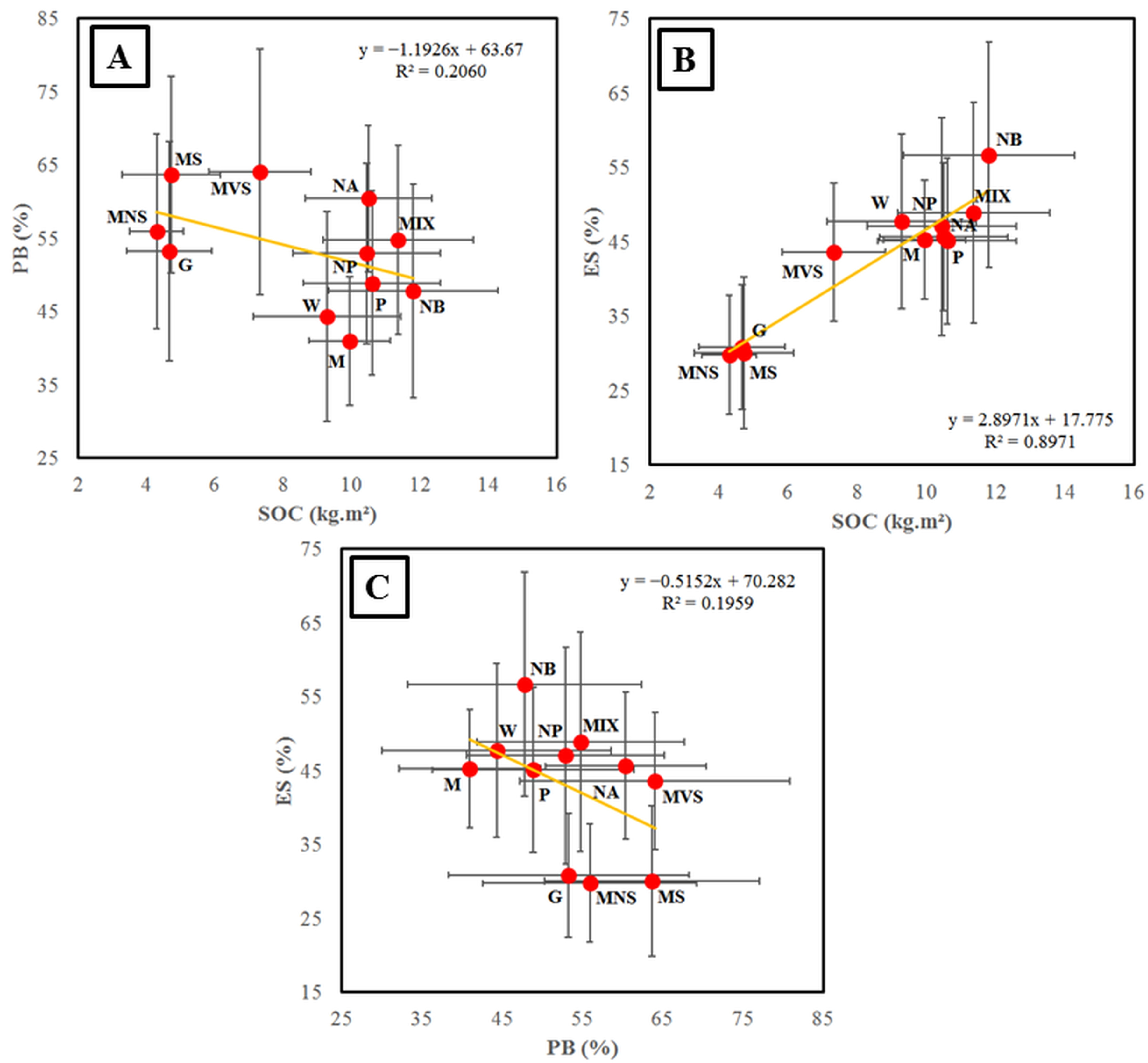
3.2. Vegetation Type Classes and their Relationships with Biodiversity, Soil Carbon, and Ecosystem Services

Pure and mixed forests presented the maximum SOC (11.3–11.8 kg C/m2), followed by peatlands (10.6 kg m−2) and deciduous Nothofagus forests (10.5 kg C/m2) (Table 3). Murtillar dwarf-shrubland and wetlands also presented higher SOC contents (9.3–10.0 kg C/m2), while the other open environments presented lower contents (<7.3 kg C/m2). The potential biodiversity was higher in some shrublands (64.1% in Mata Verde shrublands and 63.7% in mixed shrublands) and was comparable to those values found for open deciduous forests (N. antarctica forest, with 60.4%) (Table 3). N. betuloides presented lower values for forests (47.8%), which increased in mixed forests (54.8%) and N. pumilio forests (52.9%). In the other open lands, the Mata Negra Matorral thicket (55.9%) and steppe grasslands (53.3%) presented higher values compared with peatbogs (48.9%), wetlands (44.3%), and Murtillar dwarf-shrublands (41.0%). The provision of ESs presented maximum values in pure evergreen forests (56.7%); medium values in the other forest types (45.6–48.8%), some shrublands (e.g., Mata Verde shrubland and Murtillar dwarf-shrubland, 43.6–45.3%), wetlands (47.7%), and peatbogs (45.1%); and minimum values at the other shrubland types (Mata Negra Matorral thicket and mixed shrubland) and steppe grasslands (29.7–30.9%) (Table 3).
The relationships among the studied variables (SOC, PB, ES) showed some trends and separated groups depending on the VT classes (Figure 2): (i) One group with low SOC and medium-high PB values (steppe grasslands and Mata Verde shrubland–Mata Negra Matorral thicket–mixed shrublands) and a second one represented by the rest of the VT classes with high SOC content. There was a negative linear regression between these variables (R2 = 0.206). (ii) A close relationship was observed between ESs and SOC, where two groups were identified. The first group showed low values of both variables (steppe grasslands and Mata Verde shrubland–mixed shrublands) and the second one with the other VT classes with high values of both variables. The linear regression showed a strong positive relationship between the variables (R2 = 0.897). Finally, (iii) no clear relationship was detected between ESs and PB, without separation among VT classes, represented by a weak negative linear regression (R2 = 0.196).

4. Discussion

The construction of accurate and simple models and VT maps for extracting land use cover information could be highly relevant for natural resource management [53]. Field methods are a useful tool for the accurate identification and classification of VTs, but these traditional methods are challenging to implement due to personnel (expertise), logistical, and budget limitations. Remote sensing technology offers a practical and economical complement to studying VTs and land use changes within and across VTs over large areas [54] like the Patagonian region. In the present study, the classification of land cover and VTs of Santa Cruz province using multi-temporal Landsat images and climatic and topographic variables in the Google Earth Engine Platform achieved high levels of accuracy for most of the 19 land cover classes considered in the assessment. We selected the RF algorithm for VT class mapping. This classification algorithm’s success in land cover classification was also demonstrated by Sluiter [55], who investigated a wide range of vegetation classification methods in the Mediterranean for remote sensing imagery. They determined that the Random Forest and support vector machine methods showed better performances than traditional classification techniques. Also, land cover and VT maps using multi-temporal Landsat images have been used in broader environmental and ecological studies around the world [56,57,58]. We determined an Overall Accuracy of 90.4% and a Kappa coefficient of 0.87. According to Monserud and Leemans [59], Kappa coefficient values greater than approximately 0.85 indicate an excellent agreement. Classifying and mapping VTs is an important technical task for managing natural resources as vegetation provides several ESs and plays an essential role in affecting global climate change by influencing terrestrial CO2 [3,10,60]. For example, in a comprehensive review of the vegetation response to climate change, Afuye et al. [61] highlighted the importance of innovative tools in vegetation mapping based on multi-time series analyses to foster specific management programs toward ecological conservation and restoration policy.
The user’s (UA) and producer’s (PA) accuracy values for most land cover categories were higher than 0.8, highlighting a very good performance of the land use cover map. The obtained classes are very essential to characterize information on the natural environment and human activities in the region and to monitor spatial–temporal patterns. The main VTs extracted from the map were the grassland steppe (142,085 km2 representing 58.1% of the total area) and Mata Negra Matorral thicket (38,355 km2, 15.7%). Traditionally, steppe and shrubland areas present provisioning ecosystem services related to livestock production where different management proposals have been implemented [10]. Also, we highlighted the good accuracy determined for N. pumilio forest (PA = 0.966; UA = 0.977) and N. antarctica forest (PA = 0.875; UA = 0.907) for the regional use of these ecosystems. N. antarctica forests are used mainly as silvopastoral systems that combine trees and grasslands or pastures under grazing in the same unit of land, which have become an economical, ecological, and productive alternative land management practice in Patagonia [9]. Pure N. pumilio forests have been important in the region for timber production [36]. However, there was some confusion between a few classes. The results suggested a relatively high degree of confusion between shrublands and bare soil (lowest PA), where shrubland sometimes was classified as bare soil. We expect this response due to a high vegetation heterogeneity in shrublands in Patagonia at the microsite, patch (bare soil and vegetation), and patch mosaic scales, where abiotic (mainly water) factors play an important role in generating these patterns [13,14,62]. The effect of these mixing classes is most pronounced in high spatial heterogeneity ecosystems such as Mediterranean wooded grasslands and open shrublands [63]. This is a result of satellite resolution limitations related to landscape fragmentation into various patch types and ecotones. Developments in image processing techniques facilitating generalized patch delineation and transitional patterns analysis would be instrumental for a better shrubland classification, as it was addressed for the highly seasonal and heterogeneous Cerrado ecosystems [64]. Also, the bare soil class (lowest UA) in the terrain was sometimes classified as ephemeral water bodies. This is because the seasonal (dry summer and wet–cold winters) and inter-annual rainfall and evapotranspiration variability result in shallow waters (e.g., lagoons) presenting a strong dynamic of expansion and contraction of bare soils [26]. High temporal resolution over decades is needed to create robust baseline reference maps that can be used to train machine learning algorithms for monitoring and detecting changes in ephemeral water classes in complex and highly seasonal landscapes.
SOC values were higher in native forests (10.5–11.8 kg C/m2) and peatbogs (10.6 kg C/m2) compared with the other VTs. This is consistent with Peri et al. [12], who reported that SOC was higher in forests than in shrublands due to climate variables (isothermality and seasonality precipitation) and vegetation cover, as represented by the Normalized Difference Vegetation Index (NDVI). The highest SOC values found in the native forest compared with the other VTs may be due to better environmental conditions (mainly soil water availability), input of organic residues, and soil microbial biomass and activity [65]. The high values of carbon storage in peatlands in Patagonia are mainly driven by the physiological state of primary producers, the limitation of photo-assimilation by external conditions, and a low decomposition rate that is less than net primary productivity (NPP) over time [33,34].
Biodiversity is assumed to be a critical regulator of ecosystem function, ecosystem productivity, and the provision of ESs [66]. In the present study, the highest potential biodiversity occurred in shrublands (64.1% in Mata Verde and 63.7% in mixed shrublands) and N. antarctica forest (60.4%). This is consistent with Rosas et al. [67], who reported that shrublands in Southern Patagonia (Argentina) presented the highest values in shrublands followed by humid and dry steppes, where different climate (temperature, rainfall) and environmental (elevation, NDVI) drivers strongly influenced plant species distribution. According to Paruelo et al. [7], the distinct plant communities of steppes were mainly due to long-term differences in water availability, where most of the species presented similar ecological requirements (e.g., low specialization and middle marginality values). Similar to our results, for the same region, Rosas et al. [52] found higher potential biodiversity values in the N. antarctica forest associated with environmental heterogeneity in the ecotone between grasslands and mountain forests compared with other natural environments. The ecotone zone where the N. antarctica forest grows provides multiple micro-environments that allow for the survival of a higher number of species, as well as the existence of potential synergies among the species occurrence [66,68]. Besides this, multiple vegetation stratification in the N. antarctica forest and adjacent open areas (more shrubs and grasses species) promoted more species diversity than other close Nothofagus forests [6,35,36].
The provision of ESs showed maximum values in native forests (45.6–56.7%) and minimum values in the shrubland types (Mata Negra Matorral thicket and mixed shrubland) and steppe grasslands (29.7–30.9%). The highest ES values in the native forest compared with the other VTs in Southern Patagonia (Santa Cruz province) may be a result of better overall provisioning ESs such as timber from native forests [36] and livestock and firewood from silvopastoral systems [9,35]; regulating ESs such as soil carbon [12] and nitrogen content [69,70]; and cultural ESs at landscape level [70]. For example, Peri et al. [10] reported that lamb and wool production across vegetation types had the highest values in more productive N. antarctica forests (0.51 g lamb/m2/year and 0.15 g greasy wool/m2/year) than in shrublands and dry grass steppe. Martínez Pastur et al. [71], by mapping cultural ecosystem services at a regional scale in Southern Patagonia, found that native forests were important in determining the enjoyment of existence values (phytophilia phenomena) and aesthetic values related to water bodies and mountains because people preferred those landscapes in comparison with dry steppe.
The relationship among the studied variables showed that most VTs (except steppe grasslands, Mata Verde shrubland, Mata Negra Matorral thicket, and mixed shrublands) showed medium-high PB values with high SOC content. Similarly, Albuquerque et al. [72] reported that soil carbon significantly improves the performance of a biodiversity surrogate elaborated using abiotic variables to predict the presence of species. Thus, any effort to protect ecosystems with relatively high soil carbon stocks will also benefit threatened plant species. Biodiversity is also important because contributes to soil formation, thereby contributing to enhancing SOC content [73,74]. Many studies showed that higher plant diversity promotes higher litter accumulation in natural ecosystems [75,76]. In contrast, no clear relationship was detected between ESs and PB without separation among the VT classes. Furthermore, a positive relationship was observed between ESs and SOC for most VTs (except steppe grasslands and Mata Verde shrubland–mixed shrublands) with high values of both variables. Rosas et al. [51] reported that the highest ES values were related to soil nutrient stock and carbon sequestration in Southern Patagonia ecosystems. In Santa Cruz province (Argentina), the livestock provisioning ES (lamb and wool) was positively related to net carbon balance and SOC by influencing variables directly related to forage productivity [10].

5. Conclusions

This study has provided an accurate land cover and VT map (Overall Accuracy of 90.4%, Kappa coefficient of 0.87) that provides crucial information for ecological studies, biodiversity conservation, vegetation management and restoration, and regional strategic decision-making. We conclude that the VT map provides useful indicators that were integrated with SOC, biodiversity, and ecosystem services. SOC values were higher in native forests (10.5–11.8 kg C/m2) and peatbogs (10.6 kg C/m2) compared with the other VTs. The highest potential biodiversity occurred in shrublands (64.1% in Mata Verde and 63.7% in mixed shrublands) and N. antarctica forest (60.4%). The provision of ESs showed maximum values in native forests (45.6–56.7%) and minimum values in shrubland types (Mata Negra Matorral thicket and mixed shrublands) and steppe grasslands (29.7–30.9%). The relationships among the studied variables showed that most VTs showed medium-high PB values with high SOC content. Further characterization of mixing patterns between land cover classes (e.g., bare soil and ephemeral water bodies or shrublands and bare soil) requires higher resolutions and better classification methodologies than those provided by existing satellite sensor systems. Future research is needed to improve knowledge related to grazing and forest harvesting impacts on vegetation and grasslands ecosystem services.

Author Contributions

Conceptualization, P.L.P., J.G., B.D. and G.M.P.; methodology, P.L.P., J.G., B.D. and G.M.P.; software, J.G.; validation, J.G., B.D., L.A. and C.M.; formal analysis, J.G., B.D. and G.M.P.; investigation, P.L.P., J.G., B.D., L.A., C.M., F.F., R.L., J.R.-S. and G.M.P.; data curation, B.D., L.A., C.M. and F.F.; writing—original draft preparation, P.L.P., J.G., B.D. and G.M.P.; writing-review and editing, P.L.P., J.G., B.D. and G.M.P.; supervision, P.L.P., J.G. and G.M.P.; project administration, P.L.P.; funding acquisition, P.L.P. All authors have read and agreed to the published version of the manuscript.

Funding

This research was funded by the following grant: PD-E2-I038-002 (2019–2023) “Evaluación, monitoreo y manejo de la biodiversidad en sistemas agropecuarios y forestales” supported by INTA (Instituto Nacional de Tecnología Agropecuaria).

Institutional Review Board Statement

Not applicable.

Informed Consent Statement

Not applicable.

Data Availability Statement

The data and materials are available in the INTA (Argentina) repository (https://repositorio.inta.gob.ar/, accessed on 1 November 2023).

Acknowledgments

Acknowledgement is given to the researchers, technicians, students, and landowners who supported this research, without whom it would have been impossible to obtain the valuable information used in this work.

Conflicts of Interest

The authors declare no conflicts of interest. The funders had no role in the design of this study, in the collection, analyses, or interpretation of the data; in the writing of this manuscript; or in the decision to publish the results.

References

  1. Feddema, J.J. The Importance of Land-Cover Change in Simulating Future Climates. Science 2005, 310, 1674–1678. [Google Scholar] [CrossRef]
  2. Fathy, D.; Zakaly, H.M.H.; Lasheen, E.S.R.; Elsaman, R.; Alarifi, S.S.; Sami, M.; Awad, H.A.; Ene, A. Assessing geochemical and natural radioactivity impacts of Hamadat phosphatic mine through radiological indices. PLoS ONE 2023, 18, e0287422. [Google Scholar] [CrossRef]
  3. Xie, Y.; Sha, Z.; Yu, M. Remote sensing imagery in vegetation mapping: A review. J. Plant Ecol. 2008, 1, 9–23. [Google Scholar] [CrossRef]
  4. Costanza, R.; De Groot, R.; Braat, L.; Kubiszewski, I.; Fioramonti, L.; Sutton, P.; Farber, S.; Grasso, M. Twenty years of ecosystem services: How far have we come and how far do we still need to go? Ecosyst. Serv. 2017, 28, 1–16. [Google Scholar] [CrossRef]
  5. Hurskainen, P.; Adhikari, H.; Siljander, M.; Pellikka, P.K.E.; Hemp, A. Auxiliary datasets improve accuracy of object-based land use/land cover classification in heterogeneous savanna landscapes. Remote Sens. Environ. 2019, 233, e111354. [Google Scholar] [CrossRef]
  6. Oñatibia, G.R.; Aguiar, M.R. Continuous moderate grazing management promotes biomass production in Patagonian arid rangelands. J. Arid. Environ. 2016, 125, 73–79. [Google Scholar] [CrossRef]
  7. Paruelo, J.M.; Golluscio, R.A.; Guerschman, J.P.; Cesa, A.; Jouve, V.V.; Garbulsky, M.F. Regional scale relationships between ecosystem structure and functioning. The case of the Patagonian steppes. Glob. Ecol. Biogeogr. 2004, 13, 385–395. [Google Scholar] [CrossRef]
  8. Cibils, A.; Borrelli, P. Grasslands of Patagonia. In Grasslands of the World: Plant Production and Protection; Suttie, J., Reynolds, S., Batello, C., Eds.; FAO: Rome, Italy, 2005. [Google Scholar]
  9. Reque, J.A.; Sarasola, M.; Gyenge, J.; Fernández, M.E. Caracterización silvícola de ñirantales del norte de la Patagonia para la gestión forestal sostenible. Bosque 2007, 28, 33–45. [Google Scholar] [CrossRef]
  10. Peri, P.L.; Rosas, Y.M.; Rivera, E.; Martínez Pastur, G. Lamb and wool provisioning ecosystem services in Southern Patagonia. Sustainability 2021, 13, 8544. [Google Scholar] [CrossRef]
  11. Blanco, P.D.; del Valle, H.F.; Bouza, P.J.; Metternicht, G.I.; Hardtke, L.A. Ecological site classification of semiarid rangelands: Synergistic use of Landsat and Hyperion imagery. Int. J. Appl. Earth Obs. Geoinf. 2014, 29, 11–21. [Google Scholar] [CrossRef]
  12. Peri, P.L.; Rosas, Y.M.; Ladd, B.; Toledo, S.; Lasagno, R.G.; Martínez Pastur, G. Modelling soil carbon content in South Patagonia and evaluating changes according to climate, vegetation, desertification and grazing. Sustainability 2018, 10, 438. [Google Scholar] [CrossRef]
  13. Abril, A.; Villagra, P.; Noe, L. Spatiotemporal heterogeneity of soil fertility in the Central Monte desert (Argentina). J. Arid Environ. 2009, 73, 901–906. [Google Scholar] [CrossRef]
  14. Ares, J.; del Valle, H.; Bisigato, A. Detection of process related changes in plant patterns at extended spatial scales during early dryland desertification. Glob. Chang. Biol. 2003, 9, 1643–1659. [Google Scholar] [CrossRef]
  15. Bisigato, A.J.; Hardtke, L.A.; del Valle, H.F.; Bouza, P.J.; Palacio, R.G. Regional-scale vegetation heterogeneity in northeastern Patagonia: Environmental and spatial components. Community Ecol. 2016, 17, 8–16. [Google Scholar] [CrossRef]
  16. Maynard, J.J.; Karl, J.W. A hyper-temporal remote sensing protocol for high-resolution mapping of ecological sites. PLoS ONE 2017, 12, e0175201. [Google Scholar] [CrossRef] [PubMed]
  17. Stumpf, F.; Schneider, M.K.; Keller, A.; Mayr, A.; Rentschler, T.; Meuli, R.G.; Schaepman, M.; Liebisch, F. Spatial monitoring of grassland management using multi-temporal satellite imagery. Ecol. Indic. 2020, 113, e106201. [Google Scholar] [CrossRef]
  18. Li, W.; Dong, R.; Fu, H.; Wang, J.; Yu, L.; Gong, P. Integrating Google Earth imagery with Landsat data to improve 30-m resolutionland cover mapping. Remote Sens. Environ. 2020, 237, e111563. [Google Scholar] [CrossRef]
  19. Koskinen, J.; Leinonen, U.; Vollrath, A.; Ortmann, A.; Lindquist, E.; d’Annunzio, R.; Pekkarinen, A.; Käyhkö, N. Participatory mapping of forest plantations with Open Foris and Google Earth Engine. ISPRS J. Photogramm. Remote Sens. 2019, 148, 63–74. [Google Scholar] [CrossRef]
  20. Teluguntla, P.; Thenkabail, P.S.; Oliphant, A.; Xiong, J.; Gumma, M.K.; Congalton, R.G.; Yadav, K.; Huete, A. A 30-m landsatderived cropland extent product of Australia and China using random forest machine learning algorithm on Google Earth Engine cloud computing platform. ISPRS J. Photogramm. Remote Sens. 2018, 144, 325–340. [Google Scholar] [CrossRef]
  21. Adagbasa, E.G.; Mukwada, G. Mapping vegetation species succession in a mountainous grassland ecosystem using Landsat, ASTER MI, and Sentinel-2 data. PLoS ONE 2022, 17, e0256672. [Google Scholar] [CrossRef]
  22. Costanza, R.; Arge, R.; de Groot, R.; Farber, S.; Grasso, M.; Hannon, B.; Limburg, K.; Naeem, S.; Oneill, R.V.; Paruelo, J.; et al. The value of the world’s ecosystem services and natural capital. Nature 1997, 387, 253–260. [Google Scholar] [CrossRef]
  23. Millennium Ecosystem Assessment (MEA). Ecosystems and Human Well-Being: Synthesis; World Resources Institute: Washington, DC, USA, 2005. [Google Scholar]
  24. Miller, R.W.; Donahue, R.L. Soils: An Introduction to Soils and Plant Growth, 6th ed.; Prentice Hall: Englewood Cliffs, NJ, USA, 1990. [Google Scholar]
  25. Daily, G.C. Nature’s Services; Island Press: Washington, DC, USA, 1997. [Google Scholar]
  26. Pekel, J.F.; Cottam, A.; Gorelick, N.; Belward, A.S. High-resolution mapping of global surface water and its long-term changes. Nature 2016, 540, 418–422. [Google Scholar] [CrossRef] [PubMed]
  27. Mazzoni, E.; Rabassa, J. Inventario y clasificación de manifestaciones basálticas en la Patagonia mediante imágenes satelitales y SIG, provincia de Santa Cruz. Rev. Asoc. Geol. Argent. 2010, 66, 608–618. [Google Scholar]
  28. Zalazar, L.; Ferri, L.; Castro, M.; Gargantini, H.; Gimenez, M.; Pitte, P.; Ruiz, L.; Masiokas, M.; Costa, G.; Villalba, R. Spatial distribution and characteristics of Andean ice masses in Argentina: Results from the first National Glacier Inventory. J. Glaciol. 2020, 66, 938–949. [Google Scholar] [CrossRef]
  29. IGN—Instituto Geográfico Nacional. Determinación de la superficie correspondiente al territorio continental, antártico e insular de la República Argentina. In Documento Técnico IGN; Dirección Nacional de Servicios Geográficos: Buenos Aires, Argentina, 2022; p. 83. [Google Scholar]
  30. León, R.J.C.; Brand, D.; Collantes, M.; Paruelo, J.M.; Soriano, A. Grandes unidades de vegetación de la Patagonia extra andina. Ecol. Austral 1998, 8, 125–144. [Google Scholar]
  31. Roig, F.A. Growth conditions of Empetrum rubrum Vahl. ex Will. in the south of Argentina. Dendrochronologia 1988, 6, 43–59. [Google Scholar]
  32. Mazzoni, E.; Rabassa, J. Types and internal hydro-geomorphologic variability of mallines (wet-meadows) of Patagonia: Emphasis on volcanic plateaus. J. S. Am. Earth Sci. 2013, 46, 170–182. [Google Scholar] [CrossRef]
  33. Loisel, J.; Yu, Z. Holocene peatland carbon dynamics in Patagonia. Quat. Sci. Rev. 2013, 69, 125–141. [Google Scholar] [CrossRef]
  34. Clymo, R.S.; Turunen, J.; Tolonen, K. Carbon accumulation in peatland. Oikos 1998, 81, 368–388. [Google Scholar] [CrossRef]
  35. Peri, P.L.; Ormaechea, S.G. Relevamiento de los Bosques Nativos de ñire (Nothofagus antarctica) en Santa Cruz: Base para su Conservación y Manejo; INTA: Río Gallegos, Santa Cruz, Argentina, 2013. [Google Scholar]
  36. Peri, P.L.; Monelos, L.; Díaz, B.; Mattenet, F.; Huertas, L.; Bahamonde, H.; Rosas, Y.M.; Lencinas, M.V.; Cellini, J.M.; Martínez Pastur, G. Estado y usos de los Bosques Nativos de Lenga, Siempreverdes y Mixtos en Santa Cruz: Base para su Conservación y Manejo; INTA: Río Gallegos, Santa Cruz, Argentina, 2019. [Google Scholar]
  37. Veblen, T.T.; Donoso, C.; Kitzberger, Z.T.; Rebertus, A.J. Ecology of southern Chilean and Argentinian Nothofagus forests. In The Ecology and Biogeography of Nothofagus Forests; Veblen, T.T., Hill, R.S., Read, J., Eds.; Yale University Press: New Haven, CT, USA, 1996; pp. 293–353. [Google Scholar]
  38. Gorelick, N.; Hancher, M.; Dixon, M.; Ilyushchenko, S.; Thau, D.; Moore, R. Google Earth Engine: Planetary-scale geospatial analysis for everyone. Remote Sens. Environ. 2017, 202, 18–27. [Google Scholar] [CrossRef]
  39. Zhang, X.; Wu, S.; Yan, X.; Chen, Z. A global classification of vegetation based on NDVI, rainfall and temperature. Int. J. Climatol. 2017, 37, 2318–2324. [Google Scholar] [CrossRef]
  40. Hijmans, R.J.; Cameron, S.E.; Parra, J.L.; Jones, P.G.; Jarvis, A. Very high resolution interpolated climate surfaces for global land areas. Int. J. Clim. 2005, 25, 1965–1978. [Google Scholar] [CrossRef]
  41. Florinsky, I.V.; Kuryakova, G.A. Influence of topography on some vegetation cover properties. Catena 1996, 27, 123–141. [Google Scholar] [CrossRef]
  42. Tadono, T.; Ishida, H.; Oda, F.; Naito, S.; Minakawa, K.; Iwamoto, H. Precise Global DEM Generation by ALOS PRISM, ISPRS. Photogr. Remote Sen. Spat. Inf. Sci. 2014, 2–4, 71–76. [Google Scholar]
  43. Rouse, J.W.; Haas, R.H.; Schell, J.A.; Deering, D.W. Monitoring Vegetation Systems in the Great Plains with ERTS. NASA Spec. Publ. 1974, 351, 309–317. [Google Scholar]
  44. Huete, A.R.; Didan, K.; Miura, T.; Rodreguez, E.; Gao, X.; Ferreira, L. Overview of the radiometric and biophysical performance of the MODIS vegetation indices. Remote Sens. Environ. 2002, 83, 195–213. [Google Scholar] [CrossRef]
  45. Kaufman, Y.J.; Tanre, D. Atmosoherically resistant vegetation index (ARVI) for EOS-MODIS. Proc. IEEE Int. Geosci. Remote Sens. Symp. 1992, 92, 261–270. [Google Scholar] [CrossRef]
  46. Huete, A.R.; Jackson, R.D. Soil and atmosphere influences on the spectra of partial canopies. Remote Sens. Environ. 1988, 25, 89–105. [Google Scholar] [CrossRef]
  47. Shelestov, A.; Lavreniuk, M.; Kussul, N.; Novikov, A.; Skakun, S. Exploring Google Earth Engine Platform for Big Data Processing: Classification of Multi-Temporal Satellite Imagery for Crop Mapping. Front. Earth Sci. 2017, 5, e17. [Google Scholar] [CrossRef]
  48. Paruelo, J. Clasificación de Datos Espectrales. Percepción Remota y Sistemas de Información Geográfica: Sus Aplicaciones en Agronomía y Ciencias Ambientales; Hemisferio Sur: Buenos Aires, Argentina, 2014. [Google Scholar]
  49. Congalton, R.G. A Review of Assessing the Accuracy of Classifications of Remotely Sensed Data. Remote Sens. Environ. 1991, 37, 35–46. [Google Scholar] [CrossRef]
  50. Udali, A.; Lingua, E.; Persson, H.J. Assessing Forest Type and Tree Species Classification Using Sentinel-1 C-Band SAR Data in Southern Sweden. Remote Sens. 2021, 13, 3237. [Google Scholar] [CrossRef]
  51. Rosas, Y.M.; Peri, P.L.; Lencinas, M.V.; Lasagno, R.; Martínez Pastur, G. Improving the knowledge of plant potential biodiversity-ecosystem services links using maps at the regional level in Southern Patagonia. Ecol. Proc. 2021, 10, 53. [Google Scholar] [CrossRef]
  52. Rosas, Y.M.; Peri, P.L.; Martínez Pastur, G. Assessment of provisioning ecosystem services in terrestrial ecosystems of Santa Cruz province, Argentina. In Ecosystem Services in Patagonia: A Multi-Criteria Approach for an Integrated Assessment; Peri, P.L., Nahuelhual, L., Martínez Pastur, G., Eds.; Springer: Cham, Switzerland, 2021; Chapter 2; pp. 19–46. [Google Scholar]
  53. Macintyre, P.D.; Van Niekerk, A.; Dobrowolski, M.P.; Tsakalos, J.L.; Mucina, L. Impact of ecological redundancy on the performance of machine learning classifiers in vegetation mapping. Ecol. Evol. 2018, 8, 6728–6737. [Google Scholar] [CrossRef] [PubMed]
  54. Nordberg, M.L.; Evertson, J. Vegetation index differencing and linear regression for change detection in a Swedish mountain range using Landsat TM and ETM+ imagery. Land Degrad. Dev. 2003, 16, 139–149. [Google Scholar] [CrossRef]
  55. Sluiter, R. Mediterranean land cover change: Modelling and monitoring natural vegetation using GIS and remote sensing. Ned. Geogr. Stud. 2005, 333, 17–144. [Google Scholar]
  56. Aghababaei, M.; Ebrahimi, A.; Naghipour, A.A.; Asadi, E.; Verrelst, J. Vegetation types mapping using Multi-Temporal Landsat Images in the Google Earth Engine Platform. Remote Sens. 2021, 13, 4683. [Google Scholar] [CrossRef]
  57. Pech-May, F.; Aquino-Santos, R.; Rios-Toledo, G.; Posadas-Durán, J.P.F. Mapping of land cover with optical images, supervised algorithms, and Google Earth Engine. Sensors 2022, 22, 4729. [Google Scholar] [CrossRef]
  58. Marín Del Valle, T.; Jiang, P. Comparison of common classification strategies for large-scale vegetation mapping over the Google Earth Engine platform. Int. J. Appl. Earth Obs. Geoinf. 2022, 115, e103092. [Google Scholar] [CrossRef]
  59. Monserud, R.A.; Leemans, R. Comparing global vegetation maps with the Kappa statistic. Ecol. Model. 1992, 62, 275–293. [Google Scholar] [CrossRef]
  60. Xiao, X.M.; Zhang, Q.; Braswell, B.; Urbanski, S.; Boles, S.; Wofsy, S.; Moore, B., III; Ojima, D. Modeling gross primary production of temperate deciduous broadleaf forest using satellite images and climate data. Remote Sens. Environ. 2004, 91, 256–270. [Google Scholar] [CrossRef]
  61. Afuye, G.A.; Kalumba, A.M.; Orimoloye, I.R. Characterisation of vegetation response to climate change: A review. Sustainability 2021, 13, 7265. [Google Scholar] [CrossRef]
  62. Bisigato, A.J.; Bertiller, M.B. Temporal and micro-spatial patterning of seedling establishment. Consequences for patch dynamics in the southern Monte, Argentina. Plant Ecol. 2004, 174, 235–246. [Google Scholar]
  63. Friedl, M.A.; Brodley, C.E. Decision tree classification of land cover from remotely sensed data. Remote Sens. Environ. 1997, 61, 399–409. [Google Scholar] [CrossRef]
  64. Alencar, A.; Shimbo, J.Z.; Lenti, F.; Balzani Marques, C.; Zimbres, B.; Rosa, M.; Arruda, V.; Castro, I.; Fernandes Márcico Ribeiro, J.P.; Varela, V.; et al. Mapping three decades of changes in the Brazilian savanna native vegetation using Landsat data processed in the Google Earth Engine platform. Remote Sens. 2020, 12, 924. [Google Scholar] [CrossRef]
  65. Satti, P.; Mazzarino, M.J.; Gobbi, M.; Funes, F.; Roselli, L.; Fernandez, H. Soil N dynamics in relation to leaf litter quality and soil fertility in north-western Patagonian forests. J. Ecol. 2003, 91, 173–181. [Google Scholar] [CrossRef]
  66. Mori, A.S.; Lertzman, K.P.; Gustafsson, L. Biodiversity and ecosystem services in forest ecosystems: A research agenda for applied forest ecology. J. Appl. Ecol. 2017, 54, 12–27. [Google Scholar] [CrossRef]
  67. Rosas, Y.M.; Peri, P.L.; Carrasco, J.; Lencinas, M.V.; Pidgeon, A.M.; Politi, N.; Martinuzzi, S.; Martínez Pastur, G. Improving potential biodiversity and human footprint in Nothofagus forests of southern Patagonia through the spatial prioritization of their conservation values. In Spatial Modeling in Forest Resources Management; Shit, P.K., Reza, H., Das, P., Sankar Bhunia, S., Eds.; Springer: Cham, Switzerland, 2021; pp. 441–471. [Google Scholar]
  68. Antos, J. Understory plants in temperate forests. In Forests and Forest Plants; Owens, J.N., Gyde Lund, H., Eds.; Eolss Publishers Co., Ltd.: Oxford, UK, 2009; pp. 262–279. [Google Scholar]
  69. Powers, R.F. Nitrogen mineralization along an altitudinal gradient: Interactions of soil temperature, moisture, and substrate quality. For. Ecol. Manag. 1990, 30, 19–29. [Google Scholar] [CrossRef]
  70. Mazzarino, M.J.; Bertiller, M.; Sain, C.L.; Satti, P.; Coronato, F. Soil nitrogen dynamics in northeastern Patagonia steppe under different precipitation regimes. Plant Soil 1998, 202, 125–131. [Google Scholar] [CrossRef]
  71. Martínez Pastur, G.; Peri, P.L.; Lencinas, M.V.; Garcia-Llorente, M.; Martin-Lopez, B. Spatial patterns of cultural ecosystem services provision in Southern Patagonia. Landsc. Ecol. 2016, 31, 383–399. [Google Scholar] [CrossRef]
  72. Albuquerque, F.; Beier, P. Using abiotic variables to predict importance of sites for species representation. Conserv. Biol. 2015, 29, 1390–1400. [Google Scholar] [CrossRef]
  73. Canedoli, C.; Ferrè, C.; El Khair, D.A.; Comolli, R.; Liga, C.; Mazzucchelli, F.; Proietto, A.; Rota, N.; Colombo, G.; Bassano, B.; et al. Evaluation of ecosystem services in a protected mountain area: Soil organic carbon stock and biodiversity in alpine forests and grasslands. Ecosyst. Serv. 2020, 44, e101135. [Google Scholar] [CrossRef]
  74. Mace, G.M.; Norris, K.; Fitter, A.H. Biodiversity and ecosystem services: A multilayered relationship. Trends Ecol. Evol. 2012, 27, 19–26. [Google Scholar] [CrossRef] [PubMed]
  75. Lange, M.; Eisenhauer, N.; Sierra, C.A.; Bessler, H.; Engels, C.; Griffiths, R.; Mellado-Vázquez, P.; Malik, A.; Roy, J.; Scheu, S.; et al. Plant diversity increases soil microbial activity and soil carbon storage. Nat. Commun. 2015, 6, e6707. [Google Scholar] [CrossRef] [PubMed]
  76. Jastrow, J.D.; Amonette, J.E.; Bailey, V.L. Mechanisms controlling soil carbon turnover and their potential application for enhancing carbon sequestration. Clim. Chang. 2007, 80, 5–23. [Google Scholar] [CrossRef]
Figure 1. Land use cover in Santa Cruz province, South Patagonia, Argentina.
Sustainability 16 02025 g001
Figure 2. Relationships among (A) soil organic carbon content (SOC, kg m−2), (B) potential biodiversity (PB, %), and (C) ecosystem services (ESs, %) of the vegetation types in Santa Cruz (NP = Nothofagus pumilio forests, NA = N. antarctica forests, NB = N. betuloides forests, MIX = mixed forests, MVS = Mata Verde shrublands, MNS = Mata Negra Matorral thicket, MS = mixed shrublands, M = Murtillar dwarf-shrubland, W = wetlands, P = peatbogs, G = steppe grasslands). Bars indicate the standard deviation for both axes. Yellow lines represent simple linear regressions between variables.
Sustainability 16 02025 g002
Table 1. Area and percentage of land use cover in Santa Cruz province (Southern Patagonia, Argentina).
Cover ClassArea (km2)Class Percentage (%)
Permanent water bodies5427.92.22
Semi-permanent water bodies1625.80.67
Ephemeral water bodies909.30.37
Lava field70.20.03
Glaciers3484.11.43
Infrastructure224.40.09
Nothofagus pumilio forest2538.41.04
N. antarctica forest1000.50.41
N. betuloides forest84.30.03
Mixed forest104.40.04
Mata Verde shrubland183.00.07
Mata Negra Matorral thicket38,355.415.69
Mixed shrubland9103.33.72
Murtillar dwarf-shrubland702.40.29
Wetland2120.00.87
Peatbog44.50.02
Steppe grassland142,085.258.12
Outcrop rock11,205.74.58
Bare soil25,189.310.31
Total244,458100
Table 2. Confusion matrix of the main land use cover classification of Santa Cruz province, Southern Patagonia, Argentina. W: water (permanent water bodies, semi-permanent water bodies, ephemeral water bodies). LF: lava field. Gl: glacial ice. NP: Nothofagus pumilio forest. W: wetland. Sh: Shrubland (Mata Verde shrubland, Mata Negra Matorral thicket, mixed shrubland). Mu: Murtillar dwarf-shrubland. NA: N. antarctica forest. G: grassland/steppe. OR: outcrop rock. BS: bare soil. UA (%): user’s accuracy; PA (%): producer’s accuracy; CE (%): commission error; OE (%): omission error.
Field
PredictedClassesWLFGlNPWShMuNAGORBSTotalUACE
W21,527173767674328655728016922,9060.9400.060
LF052700013001631317170.7350.265
Gl200020,0713500031640021,9280.9150.085
NP00011,2812010181929011,5520.9770.023
W216003512,01244501321185675913,8200.8690.131
Sh360005737,03570459913813342,0060.8820.118
Mu200077257062176417079490.8880.112
NA100150115653490432038490.9070.093
G454014855302727272105,114697593110,8170.9490.051
OR3518285682912301493518,06028520,2070.8940.106
BS332000597039,1323132336435806114,4820.5570.443
Total25,69855620,39311,67713,30740,44974013989115,70821,3789301
PA0.8380.9480.9840.9660.9030.5600.9540.8750.9080.8450.867
OE0.1620.0520.0160.0340.0970.4400.0460.1250.0920.1550.133
Table 3. Characterization (average and standard deviation) of vegetation types in Santa Cruz province. SOC = soil organic carbon content (kg C/m2), PB = potential biodiversity (%), ESs = ecosystem services (%).
Vegetation TypeSOCPBESs
Nothofagus pumilio forest10.45 (2.16)52.9 (12.3)47.1 (14.6)
N. antarctica forest10.49 (1.85)60.4 (9.9)45.6 (9.9)
N. betuloides forest11.81 (2.48)47.8 (14.6)56.7 (15.1)
Mixed forest11.37 (2.19)54.8 (12.9)48.8 (14.8)
Mata Verde shrubland7.32 (1.50)64.1 (16.8)43.6 (9.3)
Mata Negra Matorral thicket4.30 (0.78)55.9 (13.3)29.7 (7.9)
Mixed shrublands4.72 (1.44)63.7 (13.4)30.1 (10.2)
Murtillar dwarf-shrubland9.95 (1.18)41.0 (8.8)45.3 (8.0)
Wetlands9.28 (2.16)44.3 (14.3)47.7 (11.7)
Peatbog10.60 (2.01)48.9 (12.6)45.1 (11.2)
Grassland steppe4.67 (1.24)53.3 (14.9)30.9 (8.4)
Disclaimer/Publisher’s Note: The statements, opinions and data contained in all publications are solely those of the individual author(s) and contributor(s) and not of MDPI and/or the editor(s). MDPI and/or the editor(s) disclaim responsibility for any injury to people or property resulting from any ideas, methods, instructions or products referred to in the content.

