Article

Physics-Based Modeling and Parameter Tracing for Industrial Demand-Side Management Applications: A Novel Approach

by
Dominik Leherbauer
* and
Peter Hehenberger
“Smart Mechatronics Engineering” Research Group, University of Applied Sciences Upper Austria, 4600 Wels, Austria
*
Author to whom correspondence should be addressed.
Sustainability 2024, 16(5), 1995; https://doi.org/10.3390/su16051995
Submission received: 31 December 2023 / Revised: 13 February 2024 / Accepted: 26 February 2024 / Published: 28 February 2024

Abstract

:
The transition to sustainable energy sources presents significant challenges for energy distribution and consumption systems. Specifically, the intermittent availability of renewable energy sources and the decreasing usage of fossil fuels pose challenges to energy flexibility and efficiency. An approach to tackle these challenges is demand-side management, aiming to adapt energy consumption and demand. A key requirement for demand-side management is the traceability of the energy flow among individual energy consumers. In recent years, advancements in industrial information and communication technology have provided additional potential for data acquisition. Complementary to acquired data, a physics-based modeling and analysis approach is proposed, which describes the energy consumption with physical parameters. This results in comprehensive options for monitoring actual energy consumption and planning future energy demand supporting energy efficiency and demand-response goals. To validate the proposed approach, a case study with a 3D printer covering approximately 110 h of active printing time is conducted. The medium-term study results indicate a consistent parameter trend over time, suggesting its conceptual suitability for industrial application. The approach helps to monitor energy efficiency among manufacturing assets by identifying peak loads and consumption hotspots, and provides parameters to estimate energy consumption of manufacturing processes. Results indicate up to 50% energy savings when switching the printing material and indicate further potentials.

1. Introduction

The United Nations (UN) sustainable development goals (SDG) provide an aim towards a sustainable future for humanity [1]. In particular, the goal of SDG 13 is to take urgent action to combat climate change, and its impacts have gained traction in the last few years. Also, driven by international agreements like the Paris Agreement or the European Green deal, goals have been set to limit emitted greenhouse gases. Closely related to combating climate change is UN SDG 7 to “ensure access to affordable, reliable, sustainable and modern energy for all”. In detail, the subgoals 7.1 to 7.3 state, until 2030, that universal access to reliable and modern energy services shall be granted, the share of renewable energy shall be increased substantially, and the rate of energy efficiency improvement shall be doubled [1]. Sustainable energy can be classified by technical, social, economical, environmental, and institutional dimensions, where the main sustainability goals can be summarized as energy efficiency, self-sufficiency, and low carbon intensity [2]. Thus, the clear need to utilize sustainable energy sourcing and consumption patterns surfaces.
A considerable share of energy is consumed by the industrial sector. Reports of the International Energy Agency (IEA) indicate that the industrial sector is responsible for approximately one third of energy demands and up to 45 percent of CO2 equivalent emissions [3]. To implement measures mitigating global warming until 2050, the IEA proposed several scenarios highlighting the need for energy transition. Three main synergetic strategies are proposed to close the gap with climate objectives, namely, expansion of renewable energy sources (RES), increase in energy efficiency (EE), and electrification of end uses. This is particularly driven by phasing out fossil fuels. In fact, the share of unabated fossil fuels will be less than 5% in 2050 compared with 2021’s share of 50% to reach net-zero emissions [3].
By being responsible for more than 40% of electricity consumption [4], industrial energy transition is a key factor towards a net-zero scenario. By analyzing the IEA’s net-zero energy scenario in detail, a notable detail is the different industrial sector strategies. While the strategy of the energy-intense industries, which by IEA definition comprises the steel, chemical and concrete industries, is mainly composed of alternative energy sources, e.g., hydrogen and technological advances such as carbon capture and storage, the less-energy-intense (light) industries have a different strategy, strongly aimed to increase electrification.
In combination with the rapidly increasing proportion of RES, which are mostly available intermittently, the need to have energy available at the right time surfaces. In addition to the intensively investigated approaches to energy storage technologies, however, there is also the possibility of adapting procedures and processes to the availability of energy. This results in an area of conflict between the possible additional costs of energy storage versus the financial and organizational expenditures of adaptability of procedures and processes to the energy availability.
A concept with a long history to tackle the resulting conflict is ’demand-side management’ (DSM) which emerged around 1980 to tackle a perceived long-time shortage in the energy supply [5]. The concept was first mentioned by Gellings [6] and initially included (i) peak clipping, (ii) valley filling, (iii) load shifting, (iv) strategic conservation, (v) strategic load growth, and (vi) flexible load shape as objectives. Through the years, DSM evolved by technological innovations, but also adapted to the evolving energy markets’ pricing schemes. Nowadays, DSM is commonly used to refer to the combination of energy efficiency and energy flexible, i.e., demand-response actions [7].
Current applications of demand-side management are mostly driven by financial incentives and aim to (i) improve energy efficiency and the respective energy consumption cost, (ii) mitigate load peaks or fill valleys to reduce the provision fee for the electrical connection power, (iii) shift loads in accordance to flexible spot market pricing, (iv) flexibilize loads to participate in the reserve market to receive financial compensation and (v) use on-site generation to combine effects of peak clipping and strategic conservation of grid-supplied power. The modern interpretation of DSM objectives is visualized in Figure 1.
Lund et al. [8] summarize the DSM benefits for system operators as a reduction in price peaks and the average spot price, shifting market power to consumers, postponing grid expansion, and reducing transmission and distribution losses. In combination with variable RES (VRES), DSM measures are able to achieve a 20% cost reduction, a 10% to 20% increase in VRES consumption, and a significantly reduced peak demand up to 50% [8]. A major barrier responsible for the slow adaption of DSM is the lack of information and communication technology (ICT) infrastructure, and the technological financing in combination with missing automation, as pointed out by Strbac [9] in 2008 and Kim and Shcherbakova [10] in 2011. With the ongoing roll-out of Industry 4.0 and similar concepts, the lack of ICT infrastructure is decreasing steadily and new methods to determine the DSM potentials arise. In fact, by being responsible for a major share of electricity consumption, light industry features a major potential to apply DSM in accordance with the high penetration of RES. To evaluate and apply the potentials of the wider availability of ICT hardware within the DSM objectives, a study is conducted to determine the energy consumption of industrial equipment, with the respective industrial peculiarities.
The remainder of the paper is organized as follows. Section 2 contains the state-of-the-art (SotA) and fundamentals of relevant topics. In detail, the industrial demand-side management applications are presented and energy relevant representations, modeling, and estimation of manufacturing systems are discussed, which form the foundation of the paper. Section 3 contains a methodology proposal for enhanced traceability in industrial demand-side management. In particular, the system paradigm serves as a basis to evaluate the equipments’ state, load behavior, and energy flows structurally. The proposed methodology will be demonstrated and validated in Section 4 with a case study, where a 3D printer is modeled, parametrized, and analyzed with the proposed approach. Section 5 discusses the implications, potentials, and limitations.

2. Background and State-of-the-Art

2.1. Demand-Side Management Barriers, Drivers, and Applications in the Industry

Due to its long history, DSM in the industrial sector has already been the subject of a number of studies considering the possible benefits. Multiple reviews point out the arising potentials to integrate the DSM objectives into industrial applications, by introducing operational data management. In order to operate an industrial demand-side managed plant, integrated communication systems and sensors, automated metering, and intelligent devices are necessary [7]. In 2021, Siddiquee et al. [11] identified information sharing as a key barrier for applied demand-response, which should be tackled by big data and data analytics to enable DR applications. Menghi et al. [12] analyzed energy efficiency barriers of manufacturing systems in 2019 and pointed out the opportunities introduced by Industry 4.0 and data management systems. In detail, most EE barriers are related to transparent data acquisition and structured data evaluation. In a review of energy-intense industries, Golmohamadi [13] also points out the availability of technical and market data as a key challenge to address to enable DSM applications.
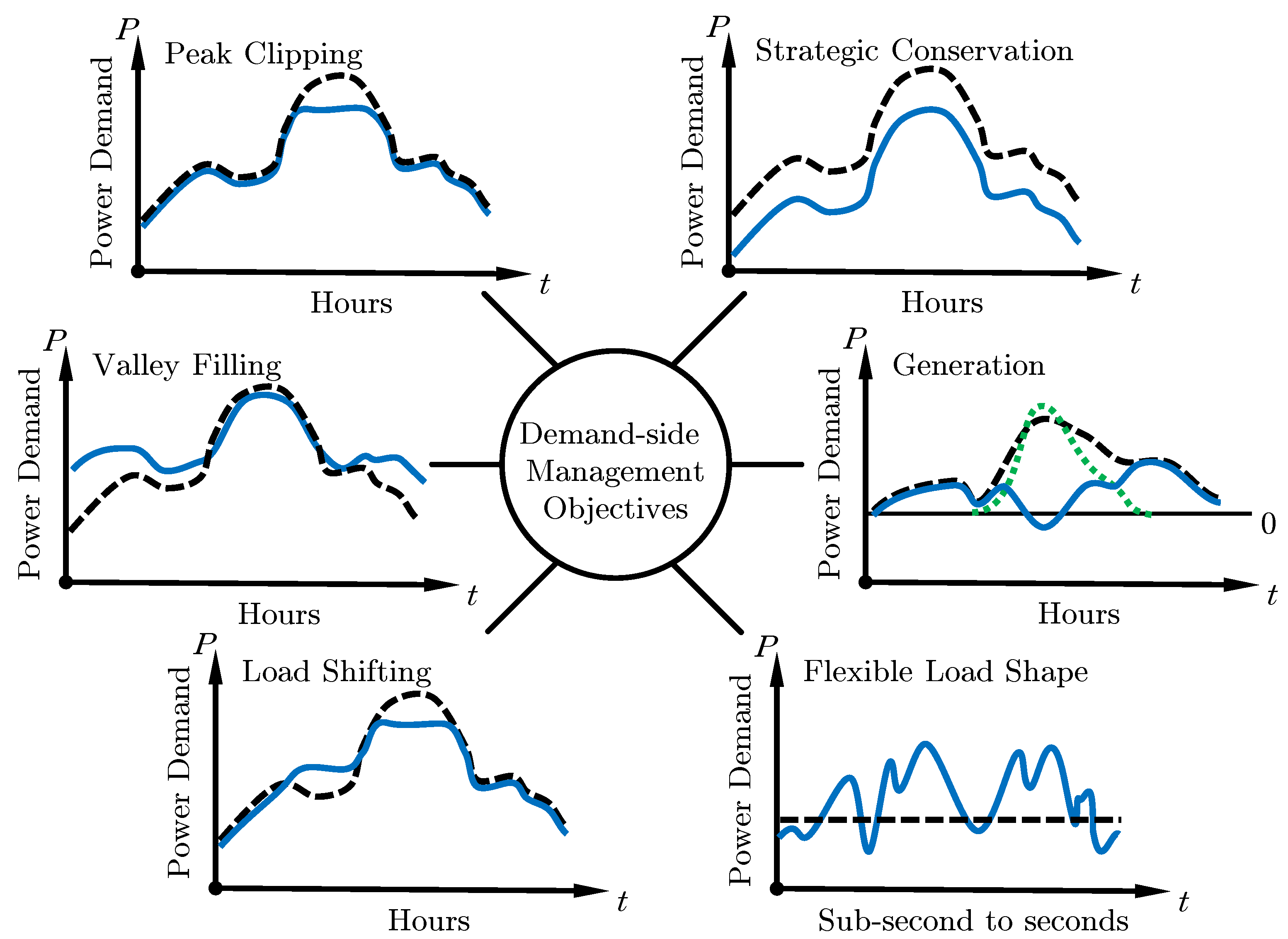
A driver to overcome the data-related barriers are savings through various incentive programs. As VRES, e.g., wind power or photovoltaic power, feature the lowest levelized cost of energy, direct savings can be achieved by utilizing these sources, with the DSM objective of generation. There is a strong correlation between electricity prices and the availability of renewables [14]. Thus, with the rising share of VRES, a rising volatility of prices in the energy exchange markets is anticipated. The rising financial and greenhouse gas emission saving potentials are seen as the key driver towards industrial DSM. There are further saving potentials enabled by flattening the load curve with valley filling or peak shaving, as the charge for the electricity connection of industrial consumers is usually dependent on the quarter-hourly maximum load. In several scientific publications, the topics of DR and EE are considered without interdependencies. Contrary, more recent publications emphasize in particular the investment in energy efficiency measures, as this can result in the reduction of peak loads and demand-response synergies [15,16,17].
The actual possibilities are largely dependent on the flexibility of loads, i.e., not all energy consumers can be switched off or controlled. Loads can be distinguished as non-interruptible, schedulable, controllable, transferable, and energy storing [18], and possible measures are chosen appropriately. It is also possible to extend the scope of industrial consumers to the building services. Dababneh et al. [19] and Jin et al. [20] used the average, respectively rated power of machines as heating sources in the HVAC planning to reduce peak power demand. For the automotive manufacturing industry, Emec et al. [21] researched the load shift and process optimization potential, and concluded a 20% energy consumption and cost savings potential. Tristán et al. [22] researched the introduction of an energy management system for three industrial systems in combination with combined heat and power, as well as a photovoltaic array for energy flexible applications. The scientific SotA thus indicates the application potential for cross-cutting and complex application scenarios.

2.2. Formal Representation of Manufacturing Systems

In their review of energy efficiency barriers Mengi et al. [12] pointed out the possibilities of data acquisition and furthermore stressed the complexity of production environments for data analysis. Thus, a structured procedure is necessary to map a physical manufacturing system formally. While conventional methods organized the data flow over several levels, namely field level, control level, supervisory level, planning, and management level, modern methods, e.g., the Industry 4.0 paradigm, use a node-based structure. While a node-based structure is able to depict complex flows, it may become congested and not able to visualize a system’s hierarchy properly. Thus, within a modern industrial environment, a system’s hierarchy and data flow have to be separated.
For the energy focus within DSM applications, an alternative representation can also be based on the energy flow. Fundamental works are based on the energetic input–output analysis by Bullard and Herendeen [23] and the embodied energy paradigm formalized by Costanza [24]. The embodied energy paradigm was adapted for a general industrial context by Rahimifard [25] and traces the energy consumption of processes to the manufacturing of goods and services. While the concept has a long history, it is still used in research and practical applications [26]. The embodied energy flow shows a structured possibility to trace energy flows over various hierarchical levels and allocate the consumption in products.
The actual process levels’ common modeling paradigm utilizes exergy principles [27] or systems engineering paradigms. Individual processes are then concisely identified by their singular inputs in the form of material and energy, and, conversely, their outputs as waste heat and products [27]. Anchored around the unit processes, Duflou et al. [28] propose a concept that aims to increase the efficiency of both energy utilization and resource management within manufacturing through the implementation of a five-level hierarchy. This hierarchy includes the device/unit process, the line/cell/multi-machine system, the plant, the multi-plant system, and the enterprise/supply chain. The unit process interfaces distinguish between inputs and outputs for various materials, energy types, and emissions.
For DR applications, dos Santos et al. [18] differentiated industrial applications on the levels’ unit process, multi-machine, and factory level. Wiendahl et al. [29] acknowledges differentiating views for changeable manufacturing, highlighting the process level as common ground for all activities. For the integration of simulation models of cyber-physical production systems from various engineering domains into meta-models, Merschak et al. [30] suggest the levels’ components, modules, systems, factories, and cyber-physical production systems.
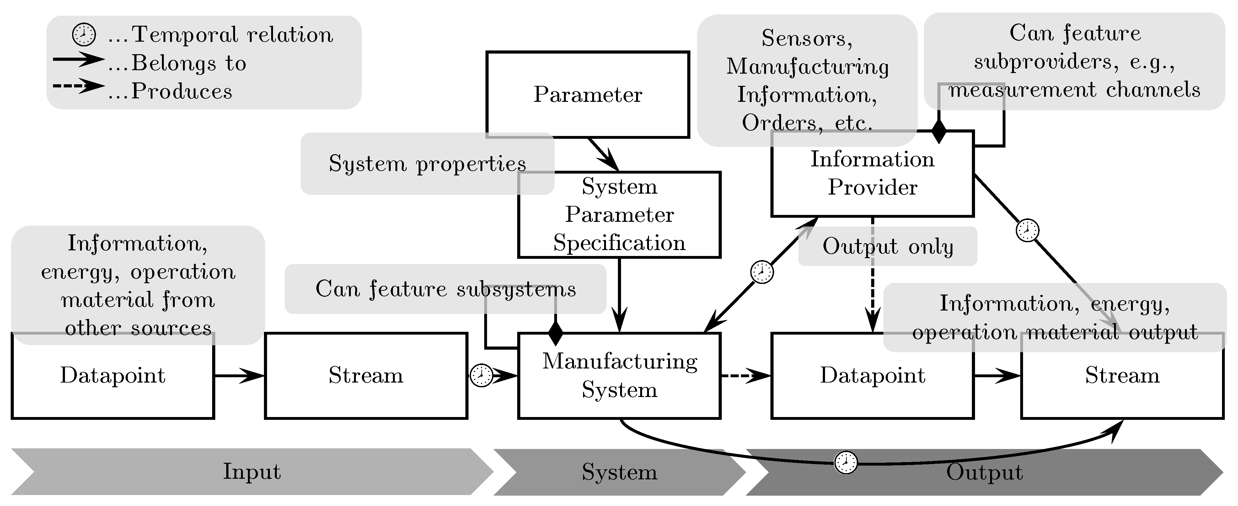
In a systems-based formalization, energy consumers such as machines are typically represented as individual systems. Within this representation, systems are represented as a block with internal properties, containing material, energy, and information as inputs and outputs [31]. Each system can feature subsystems, which also feature the respective in- and outputs. The representation is primarily focused towards the design of mechatronic systems and thus features a static hierarchy. For operational purposes, the formal model needs to constitute also dynamic information, material, and energy transfers. For example, a measurement device may be connected to different machines, a situation that cannot be represented with static flows.
The scientific SotA thus does not agree on a standardized representation of industrial systems. While there are multiple variants to visualize an industrial system, the actual depiction depends on the use case. Modern manufacturing systems require a graph-based depiction to be represented properly.

2.3. Process Load Modeling and Estimation

In the field of energy-related process load modeling and estimation techniques for manufacturing systems, various scientific efforts have been made to identify and improve prediction approaches. Schmidt et al. [32] delved into the predictive methods related to assets in the manufacturing industry, specifically highlighting the limitations of Gutowski’s approach, noting that, although it was applied to various manufacturing processes, the lack of coefficients hindered its direct use in predicting energy consumption for specific machine tools. In addition, Schmidt et al. [32] categorized machine types by complexity as simple, adjustable, single-purpose, and multi-purpose complex, and advocated the use of semi-empirical equations to model complex machines. The energy consumption monitoring patterns can be classified as constant consumption, controlled constant consumption, and variable consumption [33].
Garwood [34] highlighted different modeling methods for energy simulation tools in the manufacturing sector. Notable distinctions were made between time-driven, event-driven, continuous flow, numerical techniques, agent-driven, and co-simulation models.
Correlating with the detail of the model, the amount of data-driven varies, i.e., while most multi-machine applications, e.g., scheduling of jobs, use recorded values, unit level applications in the contrary, tend to be explainable. In fact, aside from state-based scheduling models, as introduced by Shrouf et al. [35], it is common to use the rated power or a measured average for multi-machine applications. Gong et al. [36] proposed a state-based model to elucidate the energy consumption at a machine level, specifically focusing on the power consumption of a grinding machine. Beier et al. [37] demonstrated real-time control using state-based models that rely on renewable energy sources and represent processes as discrete entities capable of switching between idle, production, and off states.
To compare the efficiencies of processes, energy key performance indicators (EnPIs) are needed. Yoon et al. [38] conducted an analysis of the specific energy consumption (SEC) as an EnPI in different manufacturing processes, and found interesting differences. The SEC is defined as energy consumption per production of one material unit, thus enabling comparisons between different manufacturing technologies. In particular, the specific energy consumption of additive processes was found to be about 100 times higher than that of bulk-forming processes. A key difference between a digital twin and a virtual testbed is the fully virtualized control [39]. Li et al. [40] introduced the concept of an energy digital twin based on a data-driven hybrid Petri net (DDPHN), and demonstrated its superiority over multiple data-driven models in simulating the energy consumption behavior of die casting. The DDPHPN reached a coefficient of determination up to 0.9662 for the needed power consumption of the casting process, demonstrating the feasibility of the data-driven methods.
In the machining domain, several publications have focused on estimating energy consumption. Liu et al. [41] proposed a model for the energy consumption of the machining process, featuring a validation error of 7.773% evaluating individual machine states, while Kara et al. [42] performed an estimation of machining energy consumption on turning and milling machines, reaching over 90% prediction accuracy. The work of Salonitis et al. [43] proposed machine disaggregation to explore energy efficiency potentials at the machine tool level by decomposing energy consumption into individual subsystems. Taken together, these efforts contribute to advancing the understanding and modeling of energy consumption in manufacturing processes.
Within the conducted literature survey, mostly white-box models, i.e., where all parameters for the calculation of the energy consumption are known, and black-box models, i.e., where the energy consumption of a system is calculated by purely data-driven methods, were applied. Grey-box models, on the contrary, which combine the existing knowledge of a system and apply data-driven methods, were not intensely studied on a process level for energy consumption estimation in industrial applications.
For other applications with grey-box models, multiple solutions exist. Fleschutz et al. [44] propose an energy optimization software framework for industrial applications on a system level, including multiple energy sources, energy storage systems and data-driven load analysis. Within the framework, multiple DR aspects can be optimized, including the peak load. Vanfretti et al. [45] introduced the RaPId toolbox to estimate FMI models for power and electric systems. ModestPy, an FMI-based python package, is a gray-box estimator, mainly applied in building services and HVAC systems [46]. For the model-predictive control of buildings, Drgona et al. [47] provide a thorough review and a unified framework, acknowledging the existing solutions and tools. Grosch et al. [48] propose an OpenAI-based framework to optimize factory operations energetically. A recent application of the parameter estimation method as an adaptive energy model was proposed by Bermeo-Ayerbe [49], and it outperformed artificial neural nets and autoregressive models with a maximum fit rate of approximately 82%, where other models had a rate less than 66%. Table 1 contains a selection of existing tools for parameter estimation of programmable objective functions, as well as simulation and data-driven models. To the best knowledge of the authors, none of the existing parameter estimation solutions evaluated contain the necessary data preparation for energy simulations on a process/unit level, suitable for the mutable nature of industrial applications.

2.4. Knowledge Gaps

The addressed scientific problem is the missing knowledge of applicability and potential of a consistent parameter estimation method for energy consumption considerations. Contrary to buildings, manufacturing entities, e.g., machines, can exhibit a significantly more complex system architecture and mostly include multiphysical phenomena. In detail, manufacturing entities feature a variety of information, energy, and material in- and outputs, which are subject to temporal changes of relations and can be comprised of subsystems, where the same characteristics apply.
The trends and developments in industrial ICT result in widespread data acquisition, while a key issue of industrial DSM is data availability. To counter the complexity of industrial systems, a holistic analysis is needed to retrieve meaningful insights from data processing [12]. In order to interpret the collected data, data-driven black-box applications, e.g., machine learning, become significantly more prevalent. Although the performance of these applications enables detailed predictions and insights, they come with the downside that they lack explainability and are often computationally expensive. White-box models, on the contrary, are poorly suited for most retrofitting applications, caused by the requirement to gather all the necessary detail information and parameters. Moreover, the considerable modeling effort to incorporate minor physical effects mostly exceeds the possible benefits for industrial applications in the operational phase. Thus, the gap in knowledge is identified as follows
  • The scientific SotA indicates no known approach to deal with the complexity and mutability of industrial systems for DSM applications, including consistent system modeling.
  • Although a variety of parameter estimation tools are known, there is no demonstrated use for the objectives of DSM. Furthermore, the potentials of identified parameters have not been evaluated within the context of industrial DSM.
By closing the gap between the missing data and appropriate evaluation, a variety of benefits are anticipated. In detail, the common energy sustainable goals would be assisted by provision of a tool to define, quantify, measure, and monitor EnPIs. Furthermore, with forecastable demands, VRES can be utilized to a higher degree to increase self-sufficiency and lower the carbon footprint. Details on the contribution to DSM are discussed in the next section.

3. Modeling and Analysis Methodology

To leverage the potential of acquired data, a modeling and analysis methodology is introduced to provide a computationally low-effort, explainable energy consumption determination for industrial environments. A simplified visualization is provided in Figure 2, which highlights the extended workflow and capabilities. As visualized, the proposed methodology aims to extend existing manufacturing systems by a structured storage of acquired data and the estimation of the energy model parameters. The results of the parameter estimation are time series of physical model parameters, e.g., electrical resistance. With the estimated parameters, additional capabilities arise, supporting DSM objectives, as detailed afterwards.
The expected results are significant enhancement in energetic traceability and the introduction of a closed-loop, which aids production planning and optimization. In detail, when using the estimated parameters for energy consumption simulations and tracking the change of parameters over time, the DSM possibilities listed in Table 2 arise.
The scope of the methodology includes the two phases of model creation and operation, where the focus lies on the energy demand model creation. As visualized in Figure 3, the energy demand model creation consists of the system and hotspot analysis, preliminary modeling, and detail modeling.
The individual phases will be presented in the rest of the section. In the system and hotspot analysis, the scope and structure of the manufacturing system is determined, and information, material, and energy flows are formally represented. The preliminary modeling phase aims to build a baseline model, representing the basic behavior of the scoped system. Within the detail modeling phase, additions to the baseline model are made to depict the actual physical behavior. The presentation of the continuous tracing and estimation concludes the section.

3.1. System and Hotspot Analysis

To create a representative model of a manufacturing entity, an initial system analysis is carried out. In order to represent the system in a formal way, the components (i) system, (ii) parameter, (iii) stream, (iv) datapoint, and (v) information provider are introduced. The link between these components is shown in Figure 4. The individual components are explained afterwards.

3.1.1. System and Parameter

Based on the existing works on the system paradigm and the literature-indicated suitability, the formal representation is anchored around the industrial systems for production. In the representation, a system represents a manufacturing entity, responsible for direct or indirect energy consumption, e.g., a machine or air-handling unit. As in the common systems’ depiction, systems can be comprised of subsystems with the limitation that a system can have zero or one parents. Additional, circularity is not allowed, e.g., System A cannot be the parent of B if B is the parent of A. Subsystems can be used to decompose complex entities into smaller, manageable parts with reduced complexity and, furthermore, introduce a hierarchy. By decomposing systems, another introduced aspect is the reusability of components, i.e., when modeling the behavior later in the workflow, standardized behavioral models can be used for common components, e.g., electrical motors or heaters.
To represent the system states and configuration, system-bound parameter specifications can be used, which feature a unit, an indicator if the parameter is known, and an initial value. Additionally, bounds can be specified for constrained parameter estimation, to constrain the estimation to physically possible ranges or a certain known numerical range. Parameter updates then only contain a reference to the parameter specification, an updated value, and a timestamp. Parameter specifications cannot be standalone and are bound to exactly one system.

3.1.2. Stream and Datapoint

To handle the linking of systems and data transmission, a concept of streams and datapoints is introduced. Fundamentally, a separation of concerns is envisaged, i.e., the streams themselves do not transmit any data but handle the temporal connections only. Datapoints, on the other hand, handle the acquired data only, but are not subject to temporal relations. Thus, as information is generally regarded as data with context, datapoints provide the data, while streams provide the context, resulting in information in the entirety.
However, a distinction must be made on the type of streams. For the energetically relevant representation, systems distinguish between physical and informational quantities. The rationale between the distinction is to enable the tracing of energy and material flows. While informational quantities are used to represent machine commands and statuses, physical quantities represent actual sensed values. Thus, a distinction solely based on the quantities unit may be ambiguous. As an example, an informational temperature setpoint would feature the same unit as a sensed temperature, but only the latter would be relevant to determine energy and material flows. A further limitation to facilitate traceability of flows exists in allowing only a single input per stream. Hence, the origin of datapoints can always be traced. Datapoints themselves contain only the minimum amount of viable data to transmit state updates. Thus, a datapoint must contain a numeric value and a unit for the state, a timestamp, and the belonging stream.

3.1.3. Information Provider

Systems are often limited in terms of data acquisition capabilities, i.e., not every relevant quantity may be available from the system itself. An example would be power metering, where machines often lack the ability to measure power consumption details, e.g., apparent and effective power. Also, systems may be dependent on external data, e.g., manufacturing instructions, to produce a specific part. To cover the additional insights and external data, information providers are introduced, acting as a container for the described cases. Information providers thus act as a container component for a wide variety of system-external elements, ranging from physical devices to virtual items. Virtual information providers may also be virtual computational nodes, which apply calculations and algorithms on acquired datapoints to provide additional states, e.g., air-cutting detection on a milling machine. Similarly to systems, information providers can feature subproviders, allowing flexible mappings. An example would be a measurement device with multiple measurement channels, as individual channels may be connected to different machines. A key difference to systems is the limitation to only output data. The rationale behind this limitation is to not impair the traceability of physical flows. Although information providers may be physically connected to the sensed stream, they should not influence or reroute them. Thus, to avoid misconceptions in flow tracing, information providers cannot be causal for a physical output and take no input.

3.1.4. System Input–Output Analysis

With all components defined, the analysis procedure can be presented. As a first step of the system analysis, a manufacturing entity, i.e., a system of interest (SoI), representing a standalone system is selected. Typically, manufacturing entities, e.g., machines, are clearly separable and allow being represented with the input–output notation. An unclear separability of the system may indicate a non-top-level system, i.e., a system with a parenting system has been selected and requires reevaluation.
After selecting a SoI, the inputs and outputs, which are necessary for operation, are analyzed. Initially, only the SoI’s environmental interactions necessary for operation are documented for energy, material, and information. The interactions include all desired and non-desired effects, and thus waste material and generated heat dissipating to the environment should be documented. The result of the system’s input–output analysis is an enumeration of external sources and sinks, which are the starting point for the system’s internal flow and hierarchy, as highlighted in the top part of Figure 5 with the gray borders.

3.1.5. Decomposition with Flow and Hierarchy Analysis

Upon researched external interfaces, the internal flows must be iteratively analyzed for information, as well as the material and energy flows between subsystems. To counter the complexity and convolution of the representation, subrepresentations (cf. bottom part of Figure 5) can be used in parallel to the overall representation (cf. top part of Figure 5). Hence, hierarchy, informational, and physical flows can be derived and constructed individually. Each flow features a direction indicating the source and sink of the respective quantity.
Notably, at this stage, information providers are not within the scope of the analysis. Hence, only systems and streams comprise the representation at this stage. By refining and detailing the graph iteratively, a directed graph results.
To determine the hierarchy and graph representation for a given system, the stream connections to information providers and systems are drawn. With the created graph, a check for consistency is necessary consisting of the hierarchy and stream check. The hierarchy check ensures for a SoI, so only one parent system exists. For all non-parent systems, the hierarchy must be resolvable without any circular relations or relations outside the SoI. The stream check includes the existence of at least one flow for each stream, i.e., no unconnected streams are allowed. In detail, the hierarchy must be checked for circular relations and the streams for at least one connection. If the consistency check fails, the system and hotspot analysis must be restarted.

3.1.6. Subsystem Composition and Hotspot Analysis

As a next step, the relevant system is analyzed for hotspots by facilitating an initial data acquisition. Thus, data acquisition devices may be needed to acquire energy-relevant data. The goal is to obtain an indication for energy-intense subsystems, as these need more detail in modeling. The suggested procedure is to screen the hierarchical levels recursively for the energy consumption shares of the parenting system. Upon reaching an insignificant share, the recursion is completed. A related analysis method is detailed in [53]. With known consumption hotspots, the individual subsystems can be composed.
An important requirement to meet for a subsystem is the standalone characteristic. The standalone characteristic is fulfilled by featuring a determinable energy flow and the subsystem not depending on environmental dependencies except those defined by in- and outputs. To create subsystems, the availability of energy-relevant in- and outputs is screened for the systems in the graph. With known subsystems meeting the standalone characteristic, the subsystems can be defined. The goal is to define as many subsystems as possible to ease modeling and validation. As noted, for common components, reusable models can be used to reduce the modeling effort.
To conclude the subsystem composition, a check is necessary, ensuring the standalone criterion is met for all subsystems. If the standalone criterion cannot be met or the hotspot analysis fails, the system and hotspot analysis needs to be restarted. Otherwise, the individual systems, in particular the detected hotspots, can be preliminarily modeled.

3.2. Preliminary Load Modeling

The aim of the preliminary load modeling stage is to create a baseline model, which robustly covers the most salient effects for a coarse prediction of the power consumption. Upon successful validation, the preliminary load model can be used as a robust baseline model, serving as a basis for model refinements, in this context referred to as supplementations, and as a baseline model for fitting error metrics for comparisons. The preliminary load modeling is carried out for every subsystem, where the result is a model definition. A model definition contains the model implementation, i.e., the analytical equations representing the equivalent behavior, and the model parameterization, i.e., the known and unknown parameters with eventual constrains.

3.2.1. Model Implementation Design

The creation of the baseline model implementation starts on the basis of previous activities. Hence, for every subsystem to model, the internal structure and eventually hotspots are known. Furthermore, the subsystem interfaces, i.e., in- and outputs for physical and informational quantities, are set and define available data and necessary outputs.
For the implementation design, the components are modeled with physical equations. As the energy relevant representation usually is not dependent on high-fidelity models, simpler differential equations are preferred, e.g., equivalent circuits for electrical components or thermal energy balances. Although theoretically possible, high-fidelity models, e.g., finite elements, should not be used, as the model estimation often takes hundreds of simulation runs.
To manage model complexity, templates for the defined equations can be defined. This allows the management of a few high-quality models, which only need to be parametrized on insertion. Especially for the baseline models, the modeling effort is greatly reduced by the usage of reusable template components.

3.2.2. Model Parameterization

Once the model is established, the specification of parameters and known values follows. Known values can be specified as constants in the model, while parameters require an initial approximation and may be bound by plausibility constraints (e.g., an electrical resistor cannot take a negative value).
The complexity of parameter estimation is inherently related to the number of parameters and the performance of the simulation. Analogous to the design of experiments methodology, an escalation in parameters requires consideration of the interrelationships between each parameter pair, resulting in a factorial increase in complexity. For the sake of parameter traceability, an analytical modeling method using physical equations is pursued. However, it is necessary to pay attention to the limitations of the analytical modeling, which, while simplifying the system, results in a coarse representation.
In addition, the resulting equations must have terms that are independent of each other. In cases where the initial observations do not provide sufficient information to define the system unambiguously, the derived parameters lack reliability. The articulation of unrelated mathematical terms may require the aggregation of multiple values; for example, an electrical resistance network may be condensed into a single parameter.

3.2.3. Validity Testing

To ensure valid models, the capabilities of the created models are tested with a defined test case. The selection of data for the test case is crucial to ensure model validity and to evaluate the strengths and weaknesses of the tested artifact appropriately. The test case should cover most system states, and transitions of multiple application scenarios and features. Upon data acquisition of the test data, the data quality must be examined for gross outliers in the data and desired frequency. When missing transitions between states, there is a chance that the parameter estimation converges to non-plausible values. Thus, it must be ensured only time series with state transitions are used.
The baseline model consists of only the assumed most contributing effects of the modeled system. If the baseline model fails to fit the estimation parameters to plausible values with a reasonable residual error, the modeling contains fundamental issues, which need to be resolved. The origins may not only be limited to the modeling quality, but may also originate from data quality or reliability, resulting in the need for reevaluation of the model definition and acquired data.
Thus, if the baseline model converges on the test case, the primary effects should be covered. If the baseline model does not reach the desired deviation, an iteration in the subsystem composition may be necessary.

3.3. Detail Modeling

If the baseline model succeeds in fitting the parameters within the set constrains, the level of detail can be increased to cover more detailed effects. While the actual modeling workflow is similar to the preliminary load modeling, the objective of detail modeling is to eradicate inaccuracies of the baseline model. In order to include only significant effects, the supplemented model can be tested against the baseline model to evaluate the change error metrics.

3.3.1. Model Supplementation

To evaluate the effect of the feature supplementation, only one feature should be added at a time and the test case rerun. Specifically, a visual analysis of discrepancies of measured versus baseline simulated data should hint at supplementation possibilities, i.e., the shortcoming of the baseline model. The actual modeling process is the same as in the baseline model creation. If new parameters are introduced, the parameters must also be set accordingly, as in the baseline model creation.

3.3.2. Baseline Testing

To validate the supplementation, the test case is run against the baseline and the supplemented models. Upon comparing the residual error of the baseline model with the extended model, error metrics can be determined, and the improvement potential can be analyzed and quantified. If the improvement is insignificant, it can be concluded the feature has no meaningful contribution to the overall model quality in relation to the added complexity and the supplementation should not be included. A significant improvement indicates that the supplementation should be included. The model supplementation is repeated until the resulting model exhibits the behavior of the scoped physical system. The overall sequence of methodological steps and decisions to create analogous models are visualized in Figure 6.

3.4. Continuous Parameter Estimation and Tracing

Upon creating and test-case validating all models, the system model creation phase is concluded, and the models are integrated into continuous tracing and estimation. Figure 7 shows the actual procedure to estimate the parameters continuously. As estimation artifacts, the baseline and the supplemented models are used. The role of the supplemented model is the provision of actual results. The role of the baseline model is to aid continuous validation by providing error metrics for a coarse estimation. To ensure the validity of models in the operation phase, several indicators can be used. As a short-term indicator for each estimation iteration, the residual error can be compared with an expected value for the supplemented and baseline models. Furthermore, the relative deviation between the baseline and supplemented estimation errors can be compared. Discrepancies show the need for action and analysis of the cause. A mid- to long-term indicator emerges when analyzing the time series of parameters. By analyzing the parameter time series, the overall stability of the estimation can be determined by analyzing the variances. Furthermore, trends can be observed and may indicate wear and tear or environmental influences. Similarly to the short-term check, a cause analysis may be initiated if the deviations are unexpected.

4. Case Study and Analysis

In order to demonstrate and validate the proposed concept, a small-scale case study was set up. Within the case study, all proposed concepts are tested and evaluated. For the case study, a 3D printer was selected, representing a multiphysical manufacturing entity composed of interconnected subsystems. The 3D printer of the type Prusa MK3S is a fused deposition modeling printer, containing one extruder, four stepper-motor-driven axes, a heated bed, two fans, and a full-fledged CNC board. By default, the 3D printer does not ship with energy metering.

4.1. Implementation Architecture Considerations and Tools

To manage the applied problems, considerable amounts of data needed to be managed. In the case of the 3D printer, approximately 60 million datapoints were collected, highlighting the need for an appropriate, database-based solution. Thus, the database schema was defined in order to map the 3D printer, data acquisition, and temporal relationships. In order to map all the elements described in the methodology, the entity-relationship diagram for TimescaleDB, shown in Figure 8, was implemented with a Python object-relational mapping (ORM). The usage of a time-series database ensures scalability of the approach and provides convenience functions to resample the acquired data to the needed simulation timesteps. By the definition of the ORM, the possibility arises to stream data to the database. Thus, acquired data from multiple sources can be merged automatically. For the implementation of the analytical models, Matlab Simulink R2023b was used as software tool. Within Matlab Simulink R2023b, subsystem templates can be defined, providing a reusable basis for common components for future modeling efforts. Within the case study, an exemplary template was created for a thermal mass, thus allowing quick modeling, by only pasting and parametrizing the template. The created models were exported as Functional Mockup Units (FMU), a standardized format for cosimulation. As a variety of other tools also support FMU, other modeling and simulation tools can also be used to create the behavioral models.
For the estimation of parameters, a Python package was implemented. For the actual parameter estimation, the optimization method, algorithm, cost function, and model interface must be defined. To deal with complex simulation models robustly, a nonlinear least-squares method was chosen, with trust-region-reflective as the algorithm from the SciPy implementation, enabling the use of parameter constrains. As cost function, the system outputs were used, comparing simulated and measured values. To minimize a bias towards bigger output values, the normalized sum squared error was used as cost function. As a normalization criterion, the output values were divided by the average value.

4.2. System and Hotspot Analysis

To obtain a representation of the 3D printer, the systems’ inputs, outputs, and subsystems are analyzed. On a system level, the energy-relevant in- and outputs are concluded by observation. The only energetic input is supplied by an alternating current plug, i.e., electric energy, and the only type of output energy is in terms of waste heat. For the information in- and outputs, the situation requires research of the printer interfaces. The Prusa MK3 is controlled via GCode commands, which can be supplied via a serial connection or SD card. A command reference for all available commands is provided by the manufacturer, and allows the specification of in- and outputs (https://help.prusa3d.com/article/prusa-firmware-specific-g-code-commands_112173 (accessed on 6 December 2023)). The information inputs mainly include:
  • Setpoints for each stepper motor axis;
  • Axis speed setpoint;
  • Temperature setpoints for each axis.
Meanwhile, the information outputs mainly include:
  • Fan speed readings;
  • Axis position readings;
  • Temperature readings for hotend, heatbed, and ambient;
  • PWM duty cycle for heatbed and hotend (from 0 to 127).
The operational material in- and output depend solely on the filament throughput. As the filament throughput is already covered by the extruder setpoints and readings, the material flow that can be derived is not declared explicitly. With most physical and informational values known, but energy flows missing, an analysis of energy flows is carried out. As a starting point for the energy flow, the outputs of the switching-mode power supply (SMPS) are traced to the logic board “Einsy RAMBo”. The schematics of the logic board show the pin assignment for the power board (https://github.com/ultimachine/Einsy-Rambo/blob/1.1a/board/ProjectOutputs/SchematicPrints_EinsyRambo_1.1a.PDF (accessed on 9 December 2023)). The SMPS features two connection ports for a constant voltage output, which are used to power (i) the heated bed, as well as (ii) stepper motors, hotend, logic, and fans separately.
To acquire measurement data in a minimal invasive way, the possibilities of using measuring devices can be summarized as follows. To determine the total active and apparent power consumption of the printer, i.e., the SMPS inputs, a power analyzer can be used. To determine the outputs, the shared output voltage and the two resulting currents can be measured by multimeters. With the determination of the use of “Keysight U1281A” multimeters with a serial connector and “Chauvin Arnoux CA8345” as a power analyzer (cf. Figure 9), the resulting graph of the flow and hierarchy analysis can be built, as shown in Figure 10.
In order to continue the system and hotspot analysis, subsystems are composited. With the connected measurement devices, the power consumption of the overall printer, the logic components, and the heatbed can be observed for a regular print to determine the hotspots. The difference between the components’ consumption and the overall printer is accounted as PSU losses, as visualized in Figure 11a. As the heatbed is not composed of subsystems, it can be determined as the major consumer, with a consumption of approximately 45%.
To obtain further indications for the logic and its subsystems, the dynamic energy consumption during the start of a print is observed, as shown in Figure 11b. Within the initial states, the active components indicate the contribution to the overall consumption. Notably, the printer control is always active when the printer is switched on and visually responsible for a constant base load. Within the preheat-extruder state, only the hotend heating is active, but not the stepper motors or hotend fan. The peak consumption of the logic components is approximately 50 watts. As the preheat state reaches a peak consumption of approximately 40 watts, the hotend heater is assumed to be the major energy consumer of the logic components. The assumption is supported by the stepper-calibration state, where the stepper motors are powered and moved to zero the relevant axes. Furthermore, the distance to the heatbed is calibrated on a number of reference points. During the stepper calibration, the hotend heating is still active to keep the desired temperature. Thus, although the stepper motors feature relatively low phase resistances of 8, and 6.5 Ω, their overall contribution to the power consumption is low. This is due to the fact that modern stepper motor drivers feature a variety of techniques, aiming to reduce power consumption and coil heating of the stepper motors. In fact, if a stepper motor is represented as an RL element in the equivalent circuit diagram, the energy consumption would be at its highest when idling if the operating voltage were simply connected up. By reducing the operation voltage and limiting currents, motor drivers counter this behavior. The overall contribution to the power consumption thus remains unknown, but the observation indicates that the stepper motors are a minor contributor.
With the print state, the operational power of the logic components peaks. Coincidentally, the extruder is actively fan cooled and starts to extrude filament, causing additional heat demand.
With the insights from the analysis of the logic behavior, the subsystems to compose can be determined. As every subsystem needs defined and measurable energy interfaces, three subsystems are defined. The first subsystem is the heatbed, taking energy setpoints or a PWM duty cycle as input and reporting the power, i.e., current demand, on the output. The second subsystem comprises the logic board, stepper motors, hotend heating, and cooling fans, and takes setpoints, i.e., the heating PWM duty cycle, as input and reports the power or current demand. The modeling efforts should be targeted at the hotend heating, as the dynamic analysis highlights a major share of power consumption within the preheating stage, where mostly no other components are active. The third subsystem is the PSU, taking the power, i.e., current demands, from the heatbed and logic as inputs and reports the active and apparent AC power on the output.
To conclude the hotspot analysis and subsystem composition, the defined subsystems are checked to feature a definable energy consumption. As each of the subsystems features a distinct definition of energy-relevant in- and outputs, the acceptance criterion is fulfilled.

4.3. Gray-Box Load Modeling and Validation

The modeling sequence and used components are typically similar to a degree. To use this characteristic, some base equations are defined and implemented in Matlab Simulink R2023b, which helps to streamline the modeling of the defined subsystems.

4.3.1. Thermal Mass

A basic element in thermodynamics is the thermal mass. Thermal mass allows the storing of thermal energy within a body and is characterized by the following equation:
Δ Q = C t h · Δ T
where Δ Q defines the added heat amount to raise the temperature by Δ T for a heat capacity of C t h . The latter be expanded as
C t h = m · c p
where m represents the body’s mass and c p the specific heat capacity. The thermal characteristics are subject to the first law of thermodynamics, i.e., for a closed system, the total energy within the system stays constant. The amount of energy can only change via heat flow to or from the system. In many applications, the specific heat capacity is not a constant but varies in temperature. In detailed simulations, this behavior has to be accounted for. However, for the approximate estimation of the energy consumption, this peculiarity is neglected.

4.3.2. Modulated Electrical Heater

A common way of adding heat is by electrical heating. For a simple electrical heater, electrical energy is converted to heat, with an efficiency degree of 1, i.e., no other effects are considered. Thus, an electrical heater can be expressed as
Δ Q = t 0 t 1 P ( t ) d t
where Δ Q defines the amount of heat added and P ( t ) the electrical power at time t. For a direct current (DC) system, the active electrical power, P ( t ) , is subject to the physical quantities current, I ( t ) , and voltage, U ( t ) , via
P ( t ) = I ( t ) · U ( t )
Usually, electrical DC systems are subject to a constant voltage or current, and either U ( t ) or I ( t ) are constants. By adding the characteristics of an electrical resistor, R, to the equation with Ohms law, stating U = R · I , all equations for non-modulated heating are known. To provide a modulation of the output power, the variable w ( t ) and constant w m a x are introduced, which control and limit output power, where w [ 0 , w m a x ] . Rewriting the equations for a modulated heating, the equations
I m o d = U ( t ) R ( t ) · w ( t ) w m a x
Δ Q m o d = t 0 t 1 U ( t ) 2 R ( t ) · w ( t ) w m a x d t
result.

4.3.3. Temperature-Dependent Electrical Resistor

In order to account for thermal effects of electrical resistors, i.e., thermistors, multiple approximations are known. In general, there is a differentiation between positive-temperature coefficients (PTC) and negative-temperature coefficients (NTC).
A PTC thermistor features an increasing resistance with rising temperature In order to account for temperature-dependent behavior over a wide temperature range, the Steinhart–Hart equation is widely used and includes three coefficients. For smaller temperature ranges, the behavior of the thermistor can be assumed as linear, introducing only one additional parameter to Ohms law, expressed as
R T ( T ) = R T 0 · ( 1 + α · Δ T ) = R T 0 + R T 0 · α · ( T T 0 )
where R T 0 is the electrical resistance at a reference temperature, T 0 , and α is the temperature coefficient, representing PTC or NTC behavior based on its sign.

4.3.4. Thermal Surface Loss

In order to account for the heat transfer between the thermodynamic systems’ boundaries, a distinction between heat conduction, convection, and thermal radiation can be made. For the 3D printer, the main assumed heat transfer is convection to the surrounding air, where the basic equation is defined as
Δ Q = t 0 t 1 h · A · Δ T d t
where Δ Q defines the amount of heat convected, h is the heat transfer coefficient, A is the convecting surface area, and Δ T is the temperature difference between surface area and surrounding fluid or gas.

4.3.5. Heated Bed

To create an analogous analytical model for the heated bed, the defined system model serves as a basis. It is known that the heated bed is driven by a pulse-width modulated (PWM) control with a constant voltage and the heatbed featuring a thermal mass to store the thermal energy. As the heatbed loses temperature over time, it is known heat is transferred, which is assumed to be solely via convection, to the surrounding air for the baseline model. Thus, the basic thermal energy balance can be stated as
Δ Q B e d ( t ) = Δ Q e l ( t ) Δ Q c o n v ( t )
where Δ Q B e d ( t ) accounts for the change of the bed’s inner energy, Δ Q e l ( t ) is the thermal energy added by the electric heating, and Δ Q c o n v ( t ) representing convectional heat losses to the environment. By substituting Δ Q B e d ( t ) with Equation (1), Δ Q e l ( t ) with Equation (6), and Δ Q c o n v ( t ) with Equation (8), the energy balance is expressed as
C t h · Δ T = t 0 t 1 U ( t ) 2 R ( t ) · w ( t ) w m a x h · A · Δ T d t
where Δ T is defined as T S u r f a c e T E n v i r o n m e n t .
With the baseline equation set, the equation can be analyzed for inputs, and known and unknown parameters. The inputs and initial conditions can be deduced from the system definition and contain w ( t ) , U, T S u r f a c e 0 and T E n v i r o n m e n t and are set at simulation runtime. The known variables contain the surface of the heatbed, approximated as a two-sided plane by A 0.25 m 2 · 0.21 m 2 · 2 and the maximum PWM input w m a x = 127 . Thus, R, C t h , and h need to be estimated. For the estimation, an initial parameter guess must be given, and constrains for lower and upper bounds can be defined. As all the parameters to be estimated physically cannot be negative, each is constrained to a positive sign and initialized by a typical value.
R = 3.84   Ω [ 0 , ] C t h = 250   J K [ 0 , ] h = 10   W m 2 K [ 0 , ]
The implemented baseline model in Matlab Simulink R2023b is visualized at the top of Figure 12 and can be tested for basic convergence. As a test case, operational printing data from three consecutive prints were used. The heated bed was heated up to 60 °C for each print and cooled down after each print, as visualized in Figure 13 at the top. When running the parameter estimation with the baseline model against the acquired measurement data, the resulting simulated outputs of current and surface temperature are visualized in Figure 13 at the second position. The stabilization of temperature confirms that the baseline model shows the basic behavior of the physical counterpart. The residual errors in Table 3 also confirm the visual observation.
Therefore, the model creation sequence can proceed with the model supplementation. The visual analysis of the baseline model output reveals a shortcoming of the baseline model, this being the decreasing current consumption in the initial heating-up period. This is assumed to be caused by the temperature-dependent behavior of the electrical heating resistance. Hence, the model supplementation is the substitution of the constant electrical resistance with a thermistor, as defined in Equation (7). The newly introduced parameter, α , is initialized with α i n i t i a l = 0.393 / K and α [ , ] resulting in no constrains. The resulting implementation is visualized in the middle of Figure 12, with the supplementation highlighted in gray.
Upon reevaluation of the test case with the supplemented model, the output curves visualized in Figure 13 and residual errors in Table 3 result. The definitions for the error metrics can be found in Appendix A. Visual inspection of the output curves reveals that the desired effect on the starting current has been reached and the residual errors are reduced slightly.
The resulting artifacts of the model supplementation are the baseline model and the model with the thermistor and an additional thermal mass. The supplemented model exhibits an adequate representation of the physical behavior, thus ending the model creation phase. Within the operational phase, the supplemented model can be continuously benchmarked against the baseline model by comparing the residual errors and estimated parameters.

4.3.6. Printer Logic, Stepper, and Extruder

The second output on the PSU supplies the control board, steppers motors, fans, and the hotend heating. As the hotspot analysis revealed, the hotend heating is assumed to be the major contributor and is thus specifically covered in the baseline model. If the baseline model converges to show the basic behavior, the assumption can be confirmed. Similarly to the heated bed, the heating is controlled by a PWM signal and heat dissipates to the environment, allowing the use of the thermal balance specified in Equation (9) as a basis. As indicated by the hotspot analysis, additional dissipation is introduced by the extrusion of filament. Thus, the thermal balance can be extended by a term Q e x t for the extrusion losses. The extrusion losses can be expressed by the added inner energy of the filament as a modified version of the thermal mass equation, where m is expressed by the mass flow. Assuming the filament to be incompressible and non-expanding yields
Δ Q = d f i l a m e n t 2 · π 4 · E s e t p o i n t · ρ · c p · Δ T
In the equation, d f i l a m e n t represents the filament diameter, E s e t p o i n t the extrusion length, and ρ the filament density.
The PWM driven heater, similarly to the heated bed, provides the current temperature as output. Additionally, the logic controller, responsible for a base load, is represented by a simple electrical resistor responsible for further power demand. With all equations set, the baseline model can be implemented, as shown at the top of Figure 14.
To carry out the baseline estimation, the known and unknown parameters must be analyzed. The density of common filament is known, with approximately ρ = 1250   k g / m 3 [54], as well as the filament’s specific heat, c f i l = 1250   J / ( k g K ) [54] and the maximum PWM signal, w m a x = 127 . However, the surface area of the hotends’ heat dissipation is difficult to determine. As both the surface and the heat dissipation represent constants in Equation (8), they are expressed as a single constant, H, as a convection coefficient. This leaves the extruder heat, C t h , the extruder heat convection coefficient, H, the extruder resistance, R e , and the controller resistance, R c , as parameters to be estimated. Each parameter is constrained and initialized with an initial guess.
R e = 14.4   Ω [ 0 , ] R c = 60   Ω [ 0 , ] C t h = 500   J K [ 0 , ] H = 0.1   W K [ 0 , ]
On execution of the baseline test, the measurement data on top of Figure 15 were used to obtain the output in the second row, with the errors in the top row of Table 4. The visual analysis of the simulation output reveals that a stable temperature is reached, and the current output already features the desired behavior in large parts of the test. Thus, the assumption of the hotends’ relation to the major part of energy consumption can be confirmed. In addition to showing the basic behavior of the physical counterpart, the baseline model also reveals the weaknesses of the model: (i) the initial and cooldown temperatures deviate, and (ii) the preheating current is excessive.
In order to mitigate (i), the forced convection of the hotend fan must be considered. The fan is not active in the initial and cooldown phases of the print and thus causes the discrepancies. Similarly to H, a fan heat convection coefficient, H f , is introduced. The forced convection is assumed to be proportional to the PWM signal. Upon reevaluation of the test case, the temperature fluctuations are reduced to a moderate level while the logic currents remain unchanged, as shown in Figure 15 and Table 4.
To mitigate (ii), the current deviations when preheating, the activity of the stepper motors is included. Previous studies found only little contribution of the stepper motor speed to the total energy consumption. Within the study of Ajay et al. [55] the total consumption varied from 46 W to 50 W for all available speeds. In the study of Nguyen et al. [56], the stepper motors were responsible for a constant load of approximately 3 W. Because of the black-box behavior of the stepper motor drivers and the insignificant impact of the stepper motors, the motors are approximated and implemented as a binary switchable load. If the deviation does not show the desired improvement, a more detailed model must be used. To implement the behavior, the modulated electrical heaters’ electrical equation can be used by limiting the maximum PWM signal to m m a x = 1 . The resulting model is presented at the bottom of Figure 14. After reevaluation of the test case, the visual analysis of Figure 15 and errors in Table 4 confirm the implementation of the desired behavior.

4.3.7. Switching Mode Power Supply

A switching mode power supply (SMPS) represents a complex dynamic system, consisting of multiple stages of conversions in order to provide a constant voltage from an alternating current within defined voltage ranges. At its core, an SMPS results in two fundamental effects, i.e., (i) the AC-DC voltage conversion with an internal loss and (ii) the addition of a reactive load. Thus, an initial approach to represent the SMPS’ behavior is the modeling of a system with an internal resistance, R i , and reactance, X i . Thus, the basic active power consumption can be expressed with output power and internal losses as
P ( t ) = ( I ( t ) D C · U D C ) + U D C 2 R i
and the respective apparent power consumption as
S ( t ) = P ( t ) 2 + Q ( t ) e l 2
where I ( t ) represent the subsystem’s current demands, U represents the DC output voltage, and Q ( t ) e l = U 2 X i . As the PSU can be simplified as a capacitive load, X i is constrained to negative values only.
R i = 50   Ω [ 0 , ] X i = 50   Ω [ , 0 ]
With the equations set, the analytical model of the PSU can be implemented, as shown at the top of Figure 16, and tested. When carrying out an initial test with the duration of several prints, the results visualized in Figure 17 and errors in Table 5 are obtained. By inspection of the coefficient of performance (R2) and the mean absolute error (MAE) of apparent power errors, the changes result in a clear improvement. Furthermore, the mean bias error (MBE) now indicates a better overall fit.
Visual analysis reveals an adequate fit and basic representation during the common operating points. However, outside the common operating points, the apparent power is grossly overestimated. Upon analyzing the relation between active and apparent power as visualized in Figure 18 an indication for improvement can be obtained by linearizing the apparent power as function of the active power. The supplementation with a linearized determination is classified as an empirical model and only loosely physics based.
The modified version of the model is visualized in Figure 16 and reevaluated against the test case. The visual results confirm the linear relationship and mitigate the deviations outside of the operating points. The errors in Table 5 also show a significant improvement.

4.4. Parameter Estimation

With models for each subsystem representing the actual physical behavior, the operational performance can be evaluated within a medium-term test. The data collected and stored in the database contain approximately 110 h of active print time. The estimation data contain a variety of different prints, i.e., the individual estimation intervals sometimes contain consecutive prints and are varied with operational setpoints of extruder and heatbed temperature. As the used power analyzer was only available at the start of the data acquisition, the SMPS’s parameters could only be estimated for seven intervals.
The total evaluation of the dataset including the supplemented and baseline models took 1 h and 50 min on a PC equipped with an Intel i5 8600k CPU and 32 GB RAM. The simulation is therefore 66 times faster than a wall clock for the 3D printer. The parameter series are visualized for the heatbed in Figure 19, for the logic in Figure 20, and for the PSU in Figure 21.
The obtained results are generally stable and the occurring fluctuations are anticipated. For the major contributing parameters towards the energy consumption, the heatbed and extruder resistances are both close to the datasheet’s nominal values of 3.4 and 14.4 Ω. All other parameters seem to be plausible and are close to the anticipated values.

4.5. DSM Potential Derivation

To demonstrate the possible uses and benefits for DSM applications, the individual possibilities are discussed. With the modus operandi, the 3D printer features limited potential to be used for valley filling, generation, or flexible load objectives. However, with the models and analysis of load curves, it is known that there is an initial peak, which may be shifted to favorable times. Additional load shift potential arises when using the defined equations to estimate the consumption for a planned print. In detail, the power consumption for various temperature settings can be calculated at the operational point. For the extruder and the heatbed, the sum of thermal flows, i.e., electric heating, and thermal losses must be zero. When inserting the latest parameters, the sensitivity of the heatbed can be determined, with 1.495 W/K for every Kelvin difference to the ambient temperature. For the extruder, the sensitivity of the natural convection was determined with 0.047 W/K, and the forced convection with the part fan, with 0.12 W/K. The melting energy of one meter of filament was determined as 3.758 J/(mK). Thus, the shifting and peak clipping potential using a different material or rescheduling prints can determine the power consumption at common operation points, as shown in Table 6. As highlighted in the table, the shifting of an ABS print job would shift over 165 W, considering the heat losses of the extruder and heatbed alone. In order to represent the energy flows visually, a cube with a side length of 33 mm was sliced, with settings for PLA and 20% infill. The slicer estimated the print time as 1 h and one minute, with 3.83 m of filament consumption. Using the resulting duration and filament, the power consumption at the operating points can be calculated for each subsystem. The results are visualized in Table 7 and Figure 22.
A striking detail is the actual minor share of physically needed thermal energy to melt the filament. In addition to this detail, for energy efficiency purposes, the heating of the bed may be adapted. With the right conditions, PLA may be printed without a heated bed or at lower temperatures, resulting in vast energy savings. Furthermore, the part-printing fan may be optimized to reduce thermal losses. However, the detail in which the 3D printer can be analyzed allows measurable decisions for future actions. Thus, the presented methodology supports transparency and explainability of energy consumption.

5. Discussion and Conclusions

5.1. Interpretation of Results

Within the case study, a novel approach was applied, which aimed to identify energy-relevant parameters of a 3D printer. The 3D printer was decomposed into the subsystems’ heatbed, logic, and power supply unit by applying the proposed methodology. For each subsystem, a behavioral model was implemented, which allowed the tracing of energy consumption among the 3D printers’ parts with grey-box models. Thus, forecasts could be created for varying process parameters and to evaluate load shift, peak clipping, and energy conservation potential. Furthermore, within the mid-term case study conducted, all parameter series obtained featured expected fluctuations, but were stable within observed estimations. For a long-term case study, eventual parameter trends or outliers should be detectable.
By comparing the error metrics obtained in the case study with previous studies, the indicated quality of the fit seems to be in the same bandwidth. However, as there was no estimation case study for a 3D printer found, existing applications researched mostly used machining applications. Notably, the aimed unique characteristic is not to outperform prediction models, but to enable the tracing and prediction of energy flows with deep insights to internals while maintaining minimal invasiveness. Interesting insights were gathered within the case study, such as the physically necessary melting energy for PLA being responsible for less than 1% of energy consumption, while heating was responsible for approximately 80% of calculated energy consumption. Energy savings of up to 50% may be possible when switching the printing material from ABS to PLA.
There are, however, residual uncertainties and limitations. One uncertainty relates to the generalizability of the results. Although there are no contradictory indicators of general suitability, tests with other machines are necessary to evaluate eventual shortcomings. An application within the machining domain would aid in evaluating the performance in comparison with existing studies. Possible threats to validity include, in particular, data quality and modeling limitations. Data quality is influenced in particular by the selection of suitable DAQs and information providers. In addition to simple deviations in the values, which occur, for example, when recording with measuring devices, the synchronization of the time stamps is particularly important with multiple data sources. Provided that the data acquisition has been configured correctly, the approach presented enables the traceable acquisition of all measurement data. If recorded data turn out to be faulty, the database-based approach makes it possible to identify the origin of the data. Thus, it is possible to determine whether other entities are affected, e.g., in the case of a faulty information provider connected to several systems.
The presented approach integrates the validation of all steps, as far as possible with little system intervention, and iterates the user to the desired result. For the validation of models, however, the validation refers exclusively to the model behavior. Hence, the conformity of the model behavior with the real behavior does not imply the conformity of the model with the real asset. The models should thus be treated as featuring the same behavior, i.e., models with analogous functionality. To overcome this limitation, the parameters of the real component may be measured with an appropriate method to overcome this limitation.

5.2. Findings and Implications

The UN SDGs aim to combat climate change and to ensure access to clean energy. Following the strategies of the IEA, it is necessary to increase the share of RES, increase EE, and electrify end uses of energy. To align the availability of RES and promote EE, DSM is a key element. According to the literature survey conducted, however, a key barrier to facilitate DSM is the availability of data. The multi-timescale observability would be a well-suited extension to facilitate DSM, as the SotA reviews pointed out transparent and interpretable energy data as a key barrier. The study conducted aimed to provide deep insights into individual industrial energy consumers, thus complementing existing data-driven approaches for load profiles on a factory or sub-distribution level.
Generally, the findings are summarized as follows. The applied approach enhances the capabilities to quantify, trace, evaluate, explain, monitor, and forecast energy flow to a high level of detail at the cost of details, which could be depicted by data-driven methods. Thus, the field of application is set by the goals. While contextualized data-driven methods excel at forecasting, the approach proposed allows the derivation of potentials for DSM applications. In the context of EE, it is feasible to compare expected and actual performance. The analysis also identifies consumption hotspots that could serve as focal points for future interventions. Ongoing monitoring of parameters over time can reveal medium- and long-term wear and tear, as well as anomalies that might otherwise go unnoticed. Additionally, it is possible to estimate the energy impact resulting from process modifications early on.
There are many possibilities and applications related to demand-response aspects. Analyzing hotspots is effective in localizing peak loads within the process. With knowledge of peak loads, energy consumption can be strategically planned to avoid coinciding peaks. Additionally, this approach enables simulation and estimation of the effects of process changes. Overall, this methodology supports minimally invasive monitoring of energy flows. The approach allows quantifying EnPIs, derives measures for DR and EE actions, highlights consumption hotspots, and enables evaluations of different manufacturing technologies and parameter settings. Practical applications would help to increase EE and enable the penetration of RES, and thus aid in combating climate change in accordance with the UN SDGs. Furthermore, a scientific contribution to close the gap on data evaluation for DSM applications was made.
Within the literature survey, a notable detail is also the lack of consistent models. In detail, most applications targeting a multi-machine level use simplified models to represent machine states. As pointed out in the SotA, state-based models are mostly driven by recorded data. A further research direction would aim to close the gap from parameter estimation to the derivation of state- or event-based models. Bridging the gap between state-based models and the estimated parameters would provide consistent models in the context of interpretable models. Furthermore, although the results obtained from the 3D printer indicate applicability, an additional application within a well-established industrial application would help to evaluate the possibilities and limitations further. Further research and consistent models of the unit process level on multiple timescales could also pave the way to enable dynamic life cycle assessment [57].

Author Contributions

Conceptualization, D.L.; methodology, D.L.; software, D.L.; validation, D.L.; investigation, D.L.; writing—original draft preparation, D.L.; writing—review and editing, D.L. and P.H.; visualization, D.L.; supervision, P.H.; project administration, P.H.; funding acquisition, P.H. All authors have read and agreed to the published version of the manuscript.

Funding

This research was partially funded by the European Union’s Horizon 2020 Program grant number Grant Agreement No. 958478 “EnerMan”; State of Upper Austria’s FTI structural funding with the project “NaKuRe”; and State of Upper Austria’s dissertation program with the project “ToMoDSM”.

Data Availability Statement

Data are contained within the article.

Conflicts of Interest

The authors declare no conflicts of interest.

Appendix A. Definitions

Table A1. Definition of error metrics.
MetricDefinition
MBE—Mean Bias Error 1 N i = 1 N ( y i y ^ i )
MAE—Mean Absolute Error 1 N i = 1 N | y i y ^ i |
RMSE—Root Mean Square Error 1 N i = 1 N ( y i y ^ i ) 2
R2—Coefficient of Determination 1 i = 1 n ( y i y ^ i ) 2 i = 1 n ( y i y ¯ i ) 2
MPE—Mean Percentage Error 100 % N i = 1 N y i y ^ i y i

References

  1. United Nations. Transforming the World: The 2030 Agenda for Sustainable Development; Technical Report; United Nations: New York, NY, USA, 2015. [Google Scholar]
  2. Iddrisu, I.; Bhattacharyya, S.C. Sustainable Energy Development Index: A Multi-Dimensional Indicator for Measuring Sustainable Energy Development. Renew. Sustain. Energy Rev. 2015, 50, 513–530. [Google Scholar] [CrossRef]
  3. International Energy Agency. World Energy Outlook 2022; IEA: Paris, France, 2022. [Google Scholar]
  4. International Energy Agency. Key World Energy Statistics 2021; Technical Report; IEA: Paris, France, 2021. [Google Scholar]
  5. Loughran, D.S.; Kulick, J. Demand-Side Management and Energy Efficiency in the United States. Energy J. 2004, 25, 21–43. [Google Scholar] [CrossRef]
  6. Gellings, C. The Concept of Demand-Side Management for Electric Utilities. Proc. IEEE 1985, 73, 1468–1470. [Google Scholar] [CrossRef]
  7. Siano, P. Demand Response and Smart Grids—A Survey. Renew. Sustain. Energy Rev. 2014, 30, 461–478. [Google Scholar] [CrossRef]
  8. Lund, P.D.; Lindgren, J.; Mikkola, J.; Salpakari, J. Review of Energy System Flexibility Measures to Enable High Levels of Variable Renewable Electricity. Renew. Sustain. Energy Rev. 2015, 45, 785–807. [Google Scholar] [CrossRef]
  9. Strbac, G. Demand Side Management: Benefits and Challenges. Energy Policy 2008, 36, 4419–4426. [Google Scholar] [CrossRef]
  10. Kim, J.H.; Shcherbakova, A. Common Failures of Demand Response. Energy 2011, 36, 873–880. [Google Scholar] [CrossRef]
  11. Siddiquee, S.M.S.; Howard, B.; Bruton, K.; Brem, A.; O’Sullivan, D.T.J. Progress in Demand Response and It’s Industrial Applications. Front. Energy Res. 2021, 9, 673176. [Google Scholar] [CrossRef]
  12. Menghi, R.; Papetti, A.; Germani, M.; Marconi, M. Energy Efficiency of Manufacturing Systems: A Review of Energy Assessment Methods and Tools. J. Clean. Prod. 2019, 240, 118276. [Google Scholar] [CrossRef]
  13. Golmohamadi, H. Demand-Side Flexibility in Power Systems: A Survey of Residential, Industrial, Commercial, and Agricultural Sectors. Sustainability 2022, 14, 7916. [Google Scholar] [CrossRef]
  14. Suomalainen, K.; Pritchard, G.; Sharp, B.; Yuan, Z.; Zakeri, G. Correlation Analysis on Wind and Hydro Resources with Electricity Demand and Prices in New Zealand. Appl. Energy 2015, 137, 445–462. [Google Scholar] [CrossRef]
  15. Dorahaki, S.; Rashidinejad, M.; Abdollahi, A.; Mollahassani-pour, M. A Novel Two-Stage Structure for Coordination of Energy Efficiency and Demand Response in the Smart Grid Environment. Int. J. Electr. Power Energy Syst. 2018, 97, 353–362. [Google Scholar] [CrossRef]
  16. Wohlfarth, K.; Worrell, E.; Eichhammer, W. Energy Efficiency and Demand Response—Two Sides of the Same Coin? Energy Policy 2020, 137, 111070. [Google Scholar] [CrossRef]
  17. Menniti, D.; Pinnarelli, A.; Sorrentino, N.; Stella, F.; Aura, C.; Liutic, C.; Polizzi, G. A Tool to Assess the Interaction between Energy Efficiency, Demand Response, and Power System Reliability. Energies 2022, 15, 5563. [Google Scholar] [CrossRef]
  18. dos Santos, S.A.B.; Soares, J.M.; Barroso, G.C.; de Athayde Prata, B. Demand Response Application in Industrial Scenarios: A Systematic Mapping of Practical Implementation. Expert Syst. Appl. 2023, 215, 119393. [Google Scholar] [CrossRef]
  19. Dababneh, F.; Li, L.; Sun, Z. Peak Power Demand Reduction for Combined Manufacturing and HVAC System Considering Heat Transfer Characteristics. Int. J. Prod. Econ. 2016, 177, 44–52. [Google Scholar] [CrossRef]
  20. Jin, H.; Li, Z.; Sun, H.; Guo, Q.; Wang, B. Coordination on Industrial Load Control and Climate Control in Manufacturing Industry under TOU Prices. IEEE Trans. Smart Grid 2019, 10, 139–152. [Google Scholar] [CrossRef]
  21. Emec, S.; Kuschke, M.; Chemnitz, M.; Strunz, K. Potential for Demand Side Management in Automotive Manufacturing. In Proceedings of the IEEE PES ISGT Europe 2013, Lyngby, Denmark, 6–9 October 2013; pp. 1–5. [Google Scholar] [CrossRef]
  22. Tristán, A.; Heuberger, F.; Sauer, A. A Methodology to Systematically Identify and Characterize Energy Flexibility Measures in Industrial Systems. Energies 2020, 13, 5887. [Google Scholar] [CrossRef]
  23. Bullard, C.W.; Herendeen, R.A. The Energy Cost of Goods and Services. Energy Policy 1975, 3, 268–278. [Google Scholar] [CrossRef]
  24. Costanza, R. Embodied Energy and Economic Valuation. Science 1980, 210, 1219–1224. [Google Scholar] [CrossRef]
  25. Rahimifard, S.; Seow, Y.; Childs, T. Minimising Embodied Product Energy to Support Energy Efficient Manufacturing. CIRP Ann. 2010, 59, 25–28. [Google Scholar] [CrossRef]
  26. Xiong, W.; Huang, H.; Li, L.; Gan, L.; Zhu, L.; Gao, M.; Liu, Z. Embodied Energy of Parts in Sheet Metal Forming: Modeling and Application for Energy Saving in the Workshop. Int. J. Adv. Manuf. Technol. 2022, 118, 3933–3948. [Google Scholar] [CrossRef]
  27. Gutowski, T.; Dahmus, J.; Thiriez, A. Electrical Energy Requirements for Manufacturing Processes. In Proceedings of the 13th CIRP International Conference on Life Cycle Engineering, Leuven, Belgium, 31 May–2 June 2006. [Google Scholar]
  28. Duflou, J.R.; Sutherland, J.W.; Dornfeld, D.; Herrmann, C.; Jeswiet, J.; Kara, S.; Hauschild, M.; Kellens, K. Towards Energy and Resource Efficient Manufacturing: A Processes and Systems Approach. CIRP Ann. 2012, 61, 587–609. [Google Scholar] [CrossRef]
  29. Wiendahl, H.P.; ElMaraghy, H.A.; Nyhuis, P.; Zäh, M.F.; Wiendahl, H.H.; Duffie, N.; Brieke, M. Changeable Manufacturing-Classification, Design and Operation. CIRP Ann. 2007, 56, 783–809. [Google Scholar] [CrossRef]
  30. Merschak, S.; Hehenberger, P.; Witters, M.; Gadeyne, K. A Hierarchical Meta-Model for the Design of Cyber-Physical Production Systems. In Proceedings of the 2018 19th International Conference on Research and Education in Mechatronics (REM), Delft, The Netherlands, 6–7 June 2018; pp. 36–41. [Google Scholar]
  31. Hehenberger, P. Perspectives on Hierarchical Modeling in Mechatronic Design. Adv. Eng. Inform. 2014, 28, 188–197. [Google Scholar] [CrossRef]
  32. Schmidt, C.; Li, W.; Thiede, S.; Kara, S.; Herrmann, C. A Methodology for Customized Prediction of Energy Consumption in Manufacturing Industries. Int. J. Precis. Eng. Manuf.-Green Technol. 2015, 2, 163–172. [Google Scholar] [CrossRef]
  33. Gontarz, A.M.; Hampl, D.; Weiss, L.; Wegener, K. Resource Consumption Monitoring in Manufacturing Environments. Procedia CIRP 2015, 26, 264–269. [Google Scholar] [CrossRef]
  34. Garwood, T.L.; Hughes, B.R.; Oates, M.R.; O’Connor, D.; Hughes, R. A Review of Energy Simulation Tools for the Manufacturing Sector. Renew. Sustain. Energy Rev. 2018, 81, 895–911. [Google Scholar] [CrossRef]
  35. Shrouf, F.; Ordieres-Meré, J.; García-Sánchez, A.; Ortega-Mier, M. Optimizing the Production Scheduling of a Single Machine to Minimize Total Energy Consumption Costs. J. Clean. Prod. 2014, 67, 197–207. [Google Scholar] [CrossRef]
  36. Gong, X.; De Pessemier, T.; Joseph, W.; Martens, L. A Generic Method for Energy-Efficient and Energy-Cost-Effective Production at the Unit Process Level. J. Clean. Prod. 2016, 113, 508–522. [Google Scholar] [CrossRef]
  37. Beier, J.; Thiede, S.; Herrmann, C. Energy Flexibility of Manufacturing Systems for Variable Renewable Energy Supply Integration: Real-time Control Method and Simulation. J. Clean. Prod. 2017, 141, 648–661. [Google Scholar] [CrossRef]
  38. Yoon, H.S.; Lee, J.Y.; Kim, H.S.; Kim, M.S.; Kim, E.S.; Shin, Y.J.; Chu, W.S.; Ahn, S.H. A Comparison of Energy Consumption in Bulk Forming, Subtractive, and Additive Processes: Review and Case Study. Int. J. Precis. Eng. Manuf.-Green Technol. 2014, 1, 261–279. [Google Scholar] [CrossRef]
  39. Schluse, M.; Rossmann, J. From Simulation to Experimentable Digital Twins: Simulation-based Development and Operation of Complex Technical Systems. In Proceedings of the 2016 IEEE International Symposium on Systems Engineering (ISSE), Edinburgh, UK, 5 October 2016; pp. 1–6. [Google Scholar]
  40. Li, H.; Yang, D.; Cao, H.; Ge, W.; Chen, E.; Wen, X.; Li, C. Data-Driven Hybrid Petri-Net Based Energy Consumption Behaviour Modelling for Digital Twin of Energy-Efficient Manufacturing System. Energy 2022, 239, 122178. [Google Scholar] [CrossRef]
  41. Liu, F.; Xie, J.; Liu, S. A Method for Predicting the Energy Consumption of the Main Driving System of a Machine Tool in a Machining Process. J. Clean. Prod. 2015, 105, 171–177. [Google Scholar] [CrossRef]
  42. Kara, S.; Li, W. Unit Process Energy Consumption Models for Material Removal Processes. CIRP Ann. 2011, 60, 37–40. [Google Scholar] [CrossRef]
  43. Salonitis, K.; Ball, P. Energy Efficient Manufacturing from Machine Tools to Manufacturing Systems. Procedia CIRP 2013, 7, 634–639. [Google Scholar] [CrossRef]
  44. Fleschutz, M.; Bohlayer, M.; Braun, M.; Murphy, M.D. Demand Response Analysis Framework (DRAF): An Open-Source Multi-Objective Decision Support Tool for Decarbonizing Local Multi-Energy Systems. Sustainability 2022, 14, 8025. [Google Scholar] [CrossRef]
  45. Vanfretti, L.; Baudette, M.; Amazouz, A.; Bogodorova, T.; Rabuzin, T.; Lavenius, J.; Goméz-López, F.J. RaPId: A Modular and Extensible Toolbox for Parameter Estimation of Modelica and FMI Compliant Models. SoftwareX 2016, 5, 144–149. [Google Scholar] [CrossRef]
  46. Arendt, K.; Jradi, M.; Wetter, M.; Veje, C.T. ModestPy: An Open-Source Python Tool for Parameter Estimation in Functional Mock-up Units. In Proceedings of the The American Modelica Conference, Cambridge, MA, USA, 9–10 October 2018; pp. 121–130. [Google Scholar] [CrossRef]
  47. Drgoňa, J.; Arroyo, J.; Cupeiro Figueroa, I.; Blum, D.; Arendt, K.; Kim, D.; Ollé, E.P.; Oravec, J.; Wetter, M.; Vrabie, D.L.; et al. All You Need to Know about Model Predictive Control for Buildings. Annu. Rev. Control 2020, 50, 190–232. [Google Scholar] [CrossRef]
  48. Grosch, B.; Ranzau, H.; Dietrich, B.; Kohne, T.; Fuhrländer-Völker, D.; Sossenheimer, J.; Lindner, M.; Weigold, M. A Framework for Researching Energy Optimization of Factory Operations. Energy Inform. 2022, 5, 29. [Google Scholar] [CrossRef]
  49. Bermeo-Ayerbe, M.A.; Ocampo-Martinez, C.; Diaz-Rozo, J. Data-Driven Energy Prediction Modeling for Both Energy Efficiency and Maintenance in Smart Manufacturing Systems. Energy 2022, 238, 121691. [Google Scholar] [CrossRef]
  50. Bynum, M.L.; Hackebeil, G.A.; Hart, W.E.; Laird, C.D.; Nicholson, B.L.; Siirola, J.D.; Watson, J.P.; Woodruff, D.L. Pyomo—Optimization Modeling in Python; Springer Optimization and Its Applications; Springer International Publishing: Cham, Switzerland, 2021; Volume 67. [Google Scholar] [CrossRef]
  51. Lacerda, W.R.; da Andrade, L.P.C.; Oliveira, S.C.P.; Martins, S.A.M. SysIdentPy: A Python Package for System Identification Using NARMAX Models. J. Open Source Softw. 2020, 5, 2384. [Google Scholar] [CrossRef]
  52. Armenise, G.; Vaccari, M.; Di Capaci, R.B.; Pannocchia, G. An Open-Source System Identification Package for Multivariable Processes. In Proceedings of the 2018 UKACC 12th International Conference on Control (CONTROL), Sheffield, UK, 5–7 September 2018; pp. 152–157. [Google Scholar] [CrossRef]
  53. Leherbauer, D.; Hehenberger, P. Real-Time Allocation of Volatile Energy Related Emissions in Manufacturing. In Product Lifecycle Management. PLM in Transition Times: The Place of Humans and Transformative Technologies. PLM 2022. IFIP Advances in Information and Communication Technology; Springer International Publishing: Cham, Switzerland, 2023. [Google Scholar]
  54. Bute, I.; Tarasovs, S.; Vidinejevs, S.; Vevere, L.; Sevcenko, J.; Aniskevich, A. Thermal Properties of 3D Printed Products from the Most Common Polymers. Int. J. Adv. Manuf. Technol. 2023, 124, 2739–2753. [Google Scholar] [CrossRef]
  55. Ajay, J.; Rathore, A.S.; Song, C.; Zhou, C.; Xu, W. Don’t Forget Your Electricity Bills!: An Empirical Study of Characterizing Energy Consumption of 3D Printers. In Proceedings of the 7th ACM SIGOPS Asia-Pacific Workshop on Systems, Hong Kong, China, 4–5 August 2016; pp. 1–8. [Google Scholar] [CrossRef]
  56. Nguyen, N.D.; Ashraf, I.; Kim, W. Compact Model for 3D Printer Energy Estimation and Practical Energy-Saving Strategy. Electronics 2021, 10, 483. [Google Scholar] [CrossRef]
  57. Collinge, W.O.; Landis, A.E.; Jones, A.K.; Schaefer, L.A.; Bilec, M.M. Dynamic Life Cycle Assessment: Framework and Application to an Institutional Building. Int. J. Life Cycle Assess. 2013, 18, 538–552. [Google Scholar] [CrossRef]
Figure 1. Visual examples of modern demand-side management objectives.
Sustainability 16 01995 g001
Figure 2. Simplified activities and sequence overview.
Sustainability 16 01995 g002
Figure 3. Overview of the methodological procedure and necessary steps.
Sustainability 16 01995 g003
Figure 4. Data flow for an exemplary manufacturing system, where a datapoint can account for material, energy, and information data.
Sustainability 16 01995 g004
Figure 5. Derivation of the internal system hierarchy and flow tracing views by decomposition.
Sustainability 16 01995 g005
Figure 6. Flowchart for the creation of analogous models.
Sustainability 16 01995 g006
Figure 7. Schematic procedure to estimate and benchmark models.
Sustainability 16 01995 g007
Figure 8. Entity-relationship diagram for the database implementation.
Sustainability 16 01995 g008
Figure 9. Data sources and components of the 3D printer case study.
Sustainability 16 01995 g009
Figure 10. Resulting graph representation of the 3D printer’s hierarchy and streams.
Sustainability 16 01995 g010
Figure 11. Hotspot analysis results for (a) the 3D printer and (b) logic dynamics. (a) Energy consumption shares of scoped subsystems for a 3-hour print; (b) occurring power consumption and states of the logic subsystem at the start of a print.
Sustainability 16 01995 g011
Figure 12. Heatbed model implementations and evolution.
Sustainability 16 01995 g012
Figure 13. Heatbed model benchmarking and supplementation results.
Sustainability 16 01995 g013
Figure 14. Logic models.
Sustainability 16 01995 g014
Figure 15. Hotend model benchmarking and supplementation results.
Sustainability 16 01995 g015
Figure 16. PSU models.
Sustainability 16 01995 g016
Figure 17. Power supply model benchmarking and supplementation results.
Sustainability 16 01995 g017
Figure 18. Analysis of the relation between active and apparent power of the PSU with an ordinary least-squares linear regression curve.
Sustainability 16 01995 g018
Figure 19. Heatbed estimation trends.
Sustainability 16 01995 g019
Figure 20. Hotend estimation trends.
Sustainability 16 01995 g020
Figure 21. PSU estimation trends.
Sustainability 16 01995 g021
Figure 22. Sankey diagram of calculated energy flows at the operation point consumption for a print of 1 h 1 min duration with a bed temperature of 60 °C, extruder temperature of 215 °C, and ambient temperature of 25 °C.
Sustainability 16 01995 g022
Table 1. Selected solutions for parameter estimation.
SolutionLanguageModel InterfaceTypeActive Development 1Free
ModestPy [46]PythonFunctional Mockup InterfaceGrey Boxnoyes
OMSysIdentOpenModelicaOMSimulator modelsGrey Boxyesyes
Parameter Identification ToolboxMatlabSimulink modelsGrey Boxyesno
Pyomo [50]PythonPyomo Models (Python Functions)Grey or Black Boxyesyes
RaPId toolbox [45]MatlabFunctional Mockup InterfaceGrey Boxnoyes
SciPyPythonPython FunctionsGrey or Black Boxyesyes
Stats PackageRR functionsGrey or Black Boxyesyes
SysIdentPy [51]PythonNARMAX et al.Black Boxyesyes
SIPPY [52]PythonARX et al.Black Boxyesyes
1 New version released or active development within the last 12 months.
Table 2. Demand-side management contributions and opportunities with grey-box load estimations.
EfficiencyDemand-Response
Measure manufacturing entity degradationIdentify and mitigate peak loads
Quantify savings on possible upgradesIdentify shiftable loads and causalities
Measure energy and media distribution lossesSimulate impact of process variations
Simulate impact of process parameter variationsDetailed load estimations for fine-grain planning
Selection assistance, e.g., execute process on machine A or B
Table 3. Residual estimation errors for the heatbed.
Heatbed Current ErrorsHeatbed Temperature Errors
ModelMBEMAERMSER2MPEMBEMAERMSER2MPE
Baseline–0.0860.360930.577130.83017–2.278–0.216872.103992.711980.940490.226
Thermistor–0.101020.35490.572930.83263–1.302–0.104221.887132.466190.95078–0.047
Table 4. Residual estimation errors for the logic subsystem.
Logic Current ErrorsExtruder Temperature Errors
ModelMBEMAERMSER2MPEMBEMAERMSER2MPE
Baseline0.00.055870.088920.98771–4.448–14.0084226.294342.35360.6441814.431
Fan Convection0.00.055670.088910.98772–4.322–2.03417.3420111.108620.975524.122
Stepper Power0.00.025380.045380.9968–0.092–2.015897.2770611.060930.975734.099
Table 5. Residual estimation errors for the PSU.
Active Power ErrorsApparent Power Errors
ModelMBEMAERMSER2MPEMBEMAERMSER2MPE
Baseline4.228198.9811812.181210.93164–24.337–6.06420.2917923.433680.78998–11.33
Linearized0.07.5910111.423850.93987–8.9060.011.4757214.463830.91999–8.217
Table 6. Calculated power demands for selected printer components at the operating point at an ambient temperature of 25 °C.
Material and ParametersHeatbedExtruder
MaterialExtruder SetpointHeatbed SetpointNatural ConvectionNatural ConvectionForced ConvectionMelting Energy
PLA215 °C60 °C52.33 W 8.98 W 22.72 W 714.05 J / m
PETG250 °C90 °C97.19 W 10.62 W 26.91 W 845.58 J / m
ABS255 °C110 °C127.09 W 10.86 W 27.51 W 864.37 J / m
Table 7. Calculated shares of energy consumption for a print of 1 h 1 min duration with a bed temperature of 60 °C, extruder temperature of 215 °C, and ambient temperature of 25 °C started from preheated state.
ComponentEnergy Consumption
AC Energy107.14 Wh
DC Energy99.93 Wh
PSU Loss7.21 Wh
Bed Heating53.20 Wh
Logic46.72 Wh
Controller4.92 Wh
Stepper8.82 Wh
Extruder Heating32.99 Wh
Natural Convection Extruder9.13 Wh
Fan (Forced) Convection Extruder23.1 Wh
Melting Energy0.76 Wh
Disclaimer/Publisher’s Note: The statements, opinions and data contained in all publications are solely those of the individual author(s) and contributor(s) and not of MDPI and/or the editor(s). MDPI and/or the editor(s) disclaim responsibility for any injury to people or property resulting from any ideas, methods, instructions or products referred to in the content.

