Article

Convolutional Neural Network-Based Bidirectional Gated Recurrent Unit–Additive Attention Mechanism Hybrid Deep Neural Networks for Short-Term Traffic Flow Prediction

1
Institute for Key Laboratory of Traffic System, Chongqing Jiaotong University, Chongqing 400074, China
2
School of Traffic and Transportation, Chongqing Jiaotong University, Chongqing 400074, China
3
Institute for Intelligent Optimization of Comprehensive Transportation Systems, Chongqing Jiaotong University, Chongqing 400074, China
4
College of Civil Aviation, Nanjing University of Aeronautics and Astronautics, Nanjing 210016, China
5
Research Center for Transportation and International Supply Chain Management, Chongqing Jiaotong University, Chongqing 400074, China
6
Highway Service Center of Yongchuan District, Chongqing 402160, China
7
The David D. Reh School of Business, Clarkson University, Potsdam, NY 13699, USA
*
Author to whom correspondence should be addressed.
Sustainability 2024, 16(5), 1986; https://doi.org/10.3390/su16051986
Submission received: 30 January 2024 / Revised: 18 February 2024 / Accepted: 25 February 2024 / Published: 28 February 2024
(This article belongs to the Section Sustainable Transportation)

Abstract

:
To more accurately predict short-term traffic flow, this study posits a sophisticated integrated prediction model, CNN-BiGRU-AAM, based on the additive attention mechanism of a convolutional bidirectional gated recurrent unit neural network. This model seeks to enhance the precision of traffic flow prediction by integrating both historical and prospective data. Specifically, the model achieves prediction through two steps: encoding and decoding. In the encoding phase, convolutional neural networks are used to extract spatial correlations between weather and traffic flow in the input sequence, while the BiGRU model captures temporal correlations in the time series. In the decoding phase, an additive attention mechanism is introduced to weigh and fuse the encoded features. The experimental results demonstrate that the CNN-BiGRU model, coupled with the additive attention mechanism, is capable of dynamically capturing the temporal patterns of traffic flow, and the introduction of isolation forests can effectively handle data anomalies and missing values, improving prediction accuracy. Compared to benchmark models such as GRU, the CNN-BiGRU-AAM model shows significant improvement on the test set, with a 47.49 reduction in the Root Mean Square Error (RMSE), a 30.72 decrease in the Mean Absolute Error (MAE), and a 5.27% reduction in the Mean Absolute Percentage Error (MAPE). The coefficient of determination ( R 2 ) reaches 0.97, indicating the high accuracy of the CNN-BiGRU-AAM model in traffic flow prediction. It provides a good solution for short-term traffic flow with spatio-temporal features, thereby enhancing the efficiency of traffic management and planning and promoting the sustainable development of transportation.

1. Introduction

Due to swift urban population expansion and rising vehicle ownership rates, traffic congestion has become more prevalent. When road capacity fails to meet traffic demand, traffic flow fluctuates significantly. Therefore, improving the municipal transportation system has become an urgent task. Short-term traffic flow prediction forms the essence of ITS. Accurate traffic flow prediction is crucial for traffic planning and guidance, as it can help in dealing with traffic congestion in advance, managing traffic in real-time, improving traffic efficiency, enhancing road safety, and contributing to sustainable development.
Typically, traditional short-term predictions of traffic volume depend on statistical analysis and time series analysis. These methods usually use some statistical data to forecast the traffic flow at a specific time in the future, and the classic models are the historical average model [1], Autoregressive Moving Average Model (ARMA) [2], Autoregressive Integral Sliding Average Model (ARIMA) [3], Kalman filter model [4], etc. However, the traditional methods do not have high prediction accuracy for complex traffic flow data with nonlinear and uncertain characteristics. In the context of sustainable transportation development, the innovation and application of technologies such as artificial intelligence, machine learning, and deep learning, on the other hand, are an important foundation on which modern prediction methods rely. Machine learning algorithms such as Decision Trees (DTs) [5], Support Vector Machines (SVRs), and Random Forests (RFs) [6] can learn complex nonlinear relationships from traffic data; deep learning techniques such as recurrent neural networks (RNNs) [7], convolutional neural networks (CNNs) [8], etc., can capture complex relationships in time series data. The initial RNNs faced significant issues such as gradient vanishing and explosion, prompting Hochreiter et al. [9] to introduce long short-term memory (LSTM) units to overcome these problems, leading to the widespread use of recurrent neural networks represented by LSTM neural networks in the field of time series prediction. However, LSTM neural networks have issues including complex structures, too many parameters, slow convergence speed, and long training time. For this reason, Cho et al. [10] 2014 proposed the gated recurrent unit (GRU) neural network, which has faster convergence speed, and used it for machine translation. Since then, GRU neural networks have been widely utilized, and scholars in the field of transportation have utilized them for short-term traffic flow prediction [11,12], travel time prediction [13,14], highway speed prediction [15], etc.
Convolutional neural networks can recognize spatial features such as traffic congestion and fluctuations in vehicle flow on roadways and are widely utilized in extracting the spatial characteristics of traffic flow. Combining the advantages of CNNs, the development of hybrid deep neural networks has attracted scholarly attention. Reza et al. [16] used a hybrid neural network algorithm combining a one-dimensional CNN and LSTM to predict traffic conditions. Lee et al. [17] extracted spatial features from bus movement sequences using a one-dimensional CNN; this study captured the temporal dependencies within subsequences using LSTM networks to anticipate bus travel times. Compared to baseline models, the combination of CNN and RNN variants in prediction models has improved model accuracy and stability, leading to their widespread application in the field of traffic. Narmadha et al. [18] applied a CNN and LSTM for forecasting short-term traffic flow within a multivariate framework. Ren et al. [19] extracted local traffic flow trend features using a 1DCNN and captured long-term trend features using RNN variants (LSTM and GRU). Building on this, Yang et al. [20] endeavored to utilize a CNN for extracting spatial information and GRU for capturing long-term sequential information, thereby constructing a hybrid deep neural network integrating a CNN and GRU. Their experimental results showed that applying this model in traffic flow prediction also demonstrated good performance and robustness. Yuan et al. [21] considered the influence of traffic conditions on traffic flow and incorporated diverse data sources, such as weather, into an input vector. They constructed an integrated predictive model utilizing a CNN and GRU, aiming to forecast traffic pattern time series more accurately. When applied to single-variable and multivariable traffic flow sequence inputs, Wang et al. [22] proposed a CNN-GRU model based on an encoder–decoder (ED) framework, and their experiments confirmed that this model structure effectively resolves the issue of error accumulation.
With the deepening of research, some scholars have noticed that it is better to use both historical and future information for prediction at the same time, and bidirectional recurrent neural networks (BRNNs) have attracted the attention of scholars; BRNNs consider both past and future temporal features to better capture the temporal information of traffic speed [23]. Zhao et al. [24] applied a BRNN for traffic flow prediction, validating its superiority in extracting the spatiotemporal features of traffic flow sequences compared to other baseline models such as RNNs, ARIMA, SVRs, and LSTM. Zhuang et al. [25] utilized a CNN and a Bidirectional Long Short-Term Memory (BILSTM) model for multistep prediction, integrating spatial features of traffic data into the BILSTM model input to extract temporal features of traffic, demonstrating improved prediction accuracy compared to the SVR and GRU models. However, due to the three gates in the hidden layer, BILSTM requires more parameters, a longer training time, and a longer fitting time. Therefore, scholars [26] have proposed using the bidirectional gated recurrent unit (BiGRU) to combine future and historical data for traffic flow prediction, aiming to enhance prediction efficiency. Ma et al. [27] integrated BiGRU into the time series and correlation of collected data, extracting deep features from convolutional and aggregation layers for model training. Additionally, researchers have also attempted to combine attention mechanisms with bidirectional recurrent neural networks for prediction. Qu et al. [28] constructed a CNN–BiLSTM–attention data-driven vehicle tracking model to forecast vehicle trajectories. Zhou et al. [29] designed a CNN-BiGRU-AM model to extract the spatiotemporal characteristics of shale oil production data, achieving efficient shale oil production forecasting. Models incorporating attention mechanisms are recognized for their high accuracy and strong generalization capabilities. Subsequently, scholars [30] proposed a neural network model called ACBiGRU and applied it to short-term traffic flow prediction, embedding attention mechanisms in convolutional neural networks to focus on convolutional layer results with distinct weights, effectively extracting the spatial features of traffic flow. Chughtai et al. [31] observed a substantial enhancement in predictive accuracy through the utilization of ensemble learning to amalgamate conventional machine learning and deep learning models.
In summary, the current research on deep neural networks for predicting using both historical and future information is relatively lacking. Furthermore, there is even less research on developing hybrid deep neural networks by combining the advantages of various prediction models, and insufficient consideration has been given to integrating and analyzing multi-source features, resulting in inadequate depth of exploration. Therefore, to compensate for the above-mentioned shortcomings, this paper develops a multi-period spatiotemporal traffic flow prediction model, CNN-BiGRU-AAM, which takes into account the influence of weather. The principal contributions are outlined below:
(1)
Adopting the concept of encoding–decoding, using CNN and BiGRU for encoding, and employing the additive attention mechanism as the decoder. Through regularization of the recurrent weights, the model becomes more robust, and, combined with the use of the isolation forest anomaly detection algorithm, can handle data missingness, anomalies, and noise, thus improving the applicability and reliability of the model.
(2)
Taking into account the complex spatial and temporal relationships between weather and traffic flow data, using a CNN to determine the spatial attributes of weather and traffic flow in the input sequence, and utilizing BiGRU to encapsulate the temporal dynamics of the input sequence. By applying the additive attention mechanism to endow the model with the capability to dynamically prioritize different components, and concatenating the above models along the feature dimension’s last axis, the accuracy of traffic flow prediction is enhanced.
(3)
By using the idea of decomposition–prediction–integration, the model’s efficacy in addressing practical traffic prediction problems is demonstrated through experiments and evaluation.

2. Methodological Overview

2.1. Convolutional Neural Networks

A one-dimensional convolutional neural network is a neural network architecture that works better for extracting features from short fixed-length inputs across an entire dataset and is usually used to process one-dimensional time series data or textual data [32]. First, convolutional operations are carried out to extract salient features within the sequence; second, a convolution kernel (or filter) is used to scan the input sequence in a sliding fashion to generate a new feature representation. For the input sequence X and the convolution kernel W, the output ξ of the convolution operation is computed in each location as follows:
ξ [ j ] = ( X · W ) [ j ] = f ( k = 0 K 1 X [ j × T s + k ] · W [ k ] + b c n n )
where ξ [ j ] represents the j th element of the output sequence resulting from the convolution operation. In Equation (1), X [ j + k ] is the j + k th element of the input sequence, where j is the current position of the convolution operation, and k denotes the offset at which the convolution kernel slides; the convolution kernel is multiplied element-by-element with a portion of the input sequence (from j to j + K 1 ) and summed to produce the j th element of the output sequence. T s is the time step; W [ k ] is the k weight of the convolution kernel, which is used to perform element-by-element multiplication with a portion of the input sequence; K is the size (or window size) of the convolution kernel; b c n n is a bias term, and f ( · ) is an activation function that introduces nonlinear properties. Popular activation functions include ReLU (Rectified Linear Unit), PReLU (Parametric ReLU), etc. [33]
Then, the feature map is reduced in size through a pooling operation, which operation not only lowers the computational complexity of the model but also extracts the most significant features. The formula for the calculation is as follows:
x [ j ] = max ( X [ j × T s : ( j + 1 ) × T s ] )
where x [ j ] is the first j element of the pooled output sequence, the feature sequence obtained through the pooling operation. In Equation (2), X [ j × T s : ( j + 1 ) × T s ] indicates that a subsequence is selected in the input sequence; the start index of this subsequence is j × T s and the end index is ( j + 1 ) × T s . This form of indexing operation is usually used for intercepting a specific part of the sequence or window.

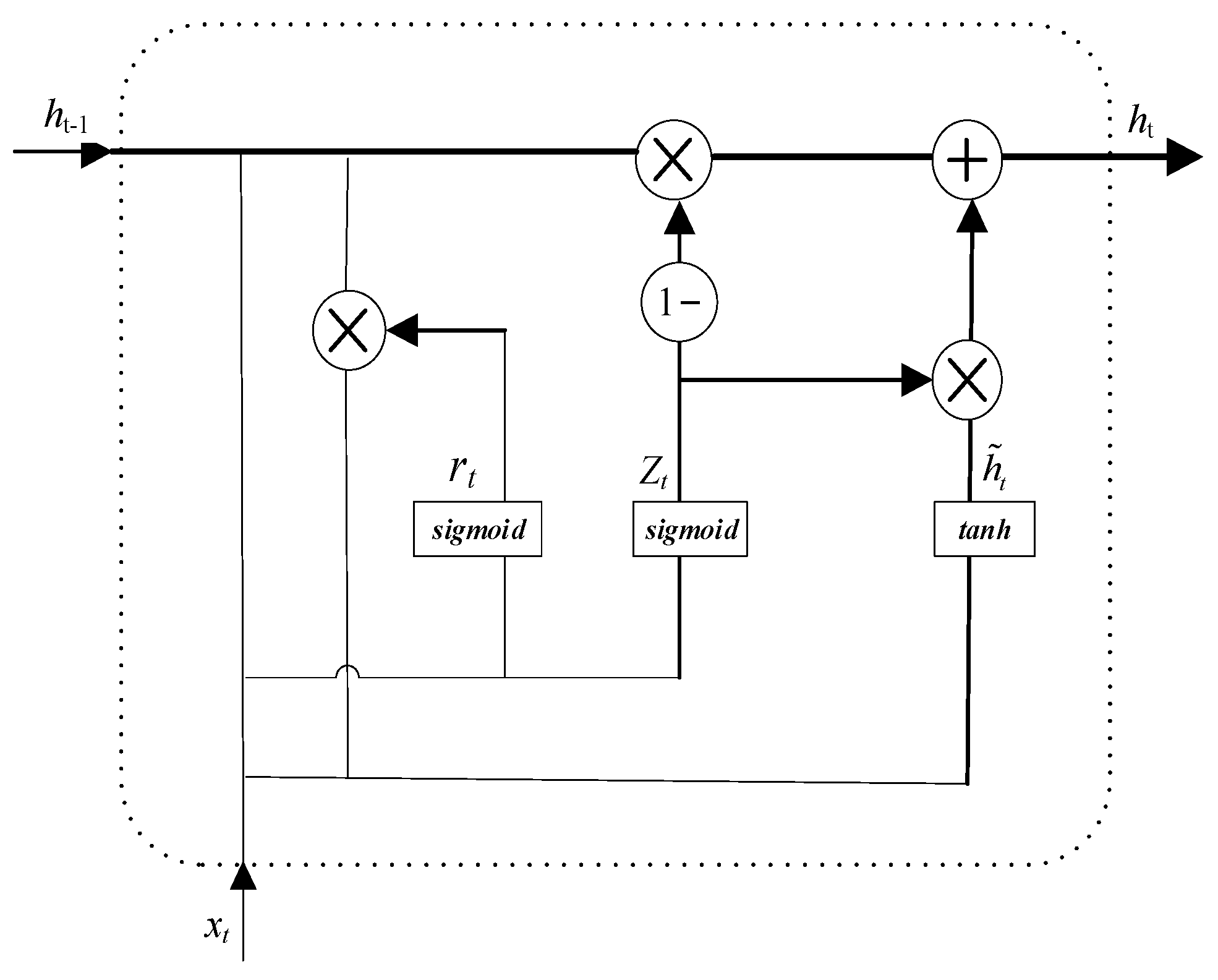
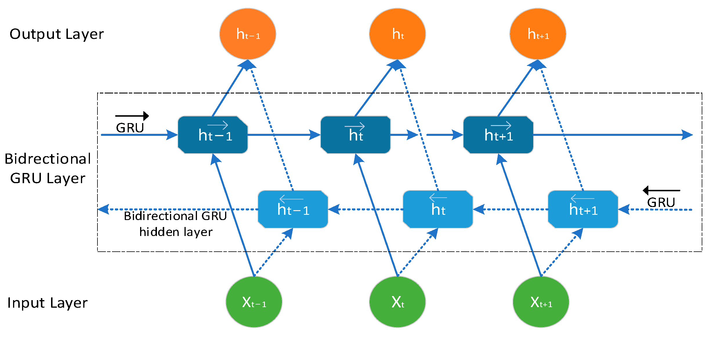
2.2. Bidirectional Gated Recurrent Unit Neural Network

GRU and LSTM both preserve important historical features by means of a “gate” structure, where the fusion of forgetting and input gates in LSTM is condensed into an update gate comprising only an update gate z and a reset gate r. GRU has no kernel state and computes the outputs directly. Figure 1 illustrates the internal architecture of a GRU.
In Figure 1, x t is the current moment input of the GRU module; h t 1 is the previous moment state; r t is the reset gate, which can be derived according to Equation (3), and is able to be used to determine the dependence degree of the candidate state h ˜ t on h t - 1 ; z t is the update gate, which is derived from Equation (4); and h t is the output candidate value after the reset gate processing. h t can be achieved by associating Equations (3)–(6).
r t = s i g m o i d ( U r h t - 1 + W r x t + b r )
z t = s i g m o i d ( U z h t - 1 + W z x t + b z )
h ˜ t = tanh ( U c ( r t h t - 1 ) + W c x t + b c )
h t = z t h t - 1 + ( 1 z t ) h ˜ t
In Equation (3), U r and W r are the weight matrices of the output of the t 1 moment and the input of the t moment to the reset gate, respectively, and b r is the bias of the reset gate; in Equation (4), U z and W z are the weight matrices of the output of the t 1 moment and the input of the t moment to the update gate, respectively, and b z denotes the bias of the update gate; and in Equation (5), b c is the bias of the candidate hidden state, and U c and W c are the weight matrices of the output of the t 1 moment and the input of the t moment to the candidate hidden state, respectively.
From Equations (3)–(6), it can be observed that the sigmoid function controls the range of values for the update and reset gates with the specified expression δ ( x ) = 1 / ( 1 + e x ) . The reset gate controls the combination of x t and h t - 1 , and the more it tends to 0, the smaller the proportion of h t 1 . The update gate z t verifies the size of h t - 1 into the current moment, the closer it gets to 1, the more the utilization of information from the preceding moment increases.
However, although the unidirectional GRU structure can collect historical information before a certain point in time, it cannot collect the before- and after-related information. BiGRU splices the outputs of two GRU layers, forward and backward, and the specific computational process can be expressed by Equations (7)–(9), and the BiGRU model is shown in Figure 2. Compared with the unidirectional GRU, the BiGRU can effectively solve the defect of having to obtain the complete relationship information between data, and it can more efficiently encapsulate the association and sequence information in the data by combining the past and future data, thus improving the model’s performance ability.
h t = G R U f ( x t , h t 1 )
h t = G R U b ( x t , h t 1 )
h t = h t h t
where h t and h t denote forward and backward GRU passes, respectively; G R U f and G R U b denote tandem combinations of forward and backward GRU functions, respectively; and ⊕ is a vector splice operation.

2.3. Additive Attention Mechanism

The additive attention mechanism (AAM) is one of the mechanisms of attention. The first use of the additive attention mechanism (or multilayer perceptron attention) was applied to sentence translation [34], and in recent years, there has been expanding utilization of this technique in the domain of image processing. It empowers the model with the ability to flexibly allocate varying weights to distinct segments within the input sequence, thereby enabling a focused analysis of crucial elements during the processing of sequence data, summing of the input features after a linear transformation, and activation of the transformed features by a sigmoid function to characterize the similarity relationship between the two features, which can effectively deal with nonlinear relationships [35]. After the CNN processes the time series features and BiGRU encodes the data, its output is accepted as input and decoded using additive attention. The following is the formula for additive attention:
y i = D e c o d e r O u t p u t ( s t , c t )
where y i denotes the decoder’s output at the time step i . In Equation (10), s t represents the hidden vector of the additive attention decoder at time step t , and y i is the output of the additive attention decoder. In Equation (11), c t is obtained by the decoder at the time step t depending on the encoder’s encoding result ( h 0 , h 1 , , h t ), which constitutes a weighted summation of the encoder’s encoding results
c t = i = 1 T a t , i h i
Regarding the weights, they are calculated as follows:
a t i = exp ( e t , i ) j = 1 T exp ( e t , j )
where the attentional weight a t i obtained from the attention score normalized by softmax, and represents the decoder’s attentional weight from the t time step to the i time step. The attention score is calculated as follows:
e t , i = v a T tanh ( W a h i + U a s t 1 )
In additive attention, the attention score is calculated through linear transformation of the encoder’s and decoder’s hidden states, followed by the application of a hyperbolic tangent function. In Equation (13), e t , i is the attention score from the decoder at the t th time step to the encoder at the i th time step; the decoding result at the current position depends on the latent state of the decoder at the previous time step s t 1 , the encoding result of the encoder at the i th time step h i . v a is the learned weight vector, and W a and U a are the learned parameter matrices in the model.

3. Prediction Method Based on CNN-BiGRU-AAM Model

Combining a CNN, BiGRU, and AAM, a CNN-BiGRU-AAM hybrid deep neural network was constructed, as shown in Figure 3.
Firstly, we leveraged a CNN to capture the spatial characteristics of traffic flow and weather in the input sequence, and combined it with a bidirectional GRU model and additive attention layer for sequence modeling. The input data underwent one-dimensional convolutional processing using convolutional kernels, followed by activation with the PReLU function, and then, we pooled layers to reduce feature dimensions and extract the most salient features. Subsequently, flattening operations were performed to transform the feature maps into one-dimensional vectors. Secondly, harnessing the power of the GRU layer to integrate historical and future information enabled the capture of temporal information in the time series. Furthermore, we applied an additive attention layer to merge the resulting feature maps produced by the CNN model, the output sequences from the GRU model, and the output from the additive attention layer to perform attention fusion. Finally, we passed this through a fully connected layer for linear transformation of the merged features, compiling the model, and producing the output.
Step 1: Outlier processing. We used the isolation forest machine learning algorithm to determine whether a data point is an outlier based on its isolation. The outlier score for a data point can be obtained by calculating the average path length of all trees in the forest and normalizing it to the range [0, 1]:
s ( x , n ) = 2 E ( h ( x ) ) C ( n )
where h ( x ) is the path length of a data point, ( n ) represents the quantity of data points, and c ( n ) is a constant derived from the mean height of a binary search tree.
Step 2: Data standardization. Using the Standard Scaler normalization method, historical traffic flow data were processed by adjusting the values of the features to have a zero mean and unit variance. The calculation is as follows:
x = x i μ ¯ σ
where μ ¯ represents the mean of the entire sample data, and σ denotes the standard deviation of the complete sample set.
Step 3: Data feature correlation analysis. In order to study the relationship between variables affecting urban traffic flow and weather, we collected quantifiable numerical weather data such as temperature, relative humidity, and visibility. Through descriptive statistical analysis and correlation heatmaps, as shown in Figure 4 we were able to discern the underlying association between weather factors and short-term traffic flow, enabling us to ascertain the extent to which weather features impact traffic volume. This analysis provides a solid foundation for developing prediction models that incorporate weather features.
Step 4: We constructed a CNN-BiGRU-AAM deep neural network. Within the context of this research article, a total of k + 1 historical short-term traffic flow data in the time period, t k , t 1 , t were employed to forecast traffic flow during the specified time period t + 1 by combining the t + 2 to t + m traffic flow data after the t + 1 time period through BiGRU; therefore, the quantity of neurons in the input layer was set to k + m , and the quantity of neurons in the output layer was set to a single unit. The quantity of neurons of CNN convolutional kernels was set to 128 and 64, respectively, and the kernel size was 2. Due to the issue of the ReLU activation function outputting zero for negative inputs, which can lead to a large number of neurons being deactivated and thereby affect the effectiveness of deep learning networks, this study adopted the PReLU activation function. PReLU introduces a learnable parameter based on ReLU, allowing negative inputs to have a small positive slope, thus preventing the complete deactivation of neurons. In PReLU, the slope coefficient for the negative part is drawn rather than being a pre-set fixed value, which helps prevent neuron death and can accelerate the model’s convergence speed. The mathematical definition of the ReLU and PReLU functions, respectively denoted as Equations (16) and (17), can be expressed as follows:
y i = x i i f x i > 0 0 i f x i 0
y i = x i i f x i > 0 a i x i i f x i 0
Figure 5 visually demonstrates the distinctions between the ReLU and RReLU activation functions.
Step 5: Parameter setting. According to the model, the connection weights and neuron bias between layers were reasonably set, and the appropriate activation function and loss function were selected. The Adam optimizer was employed while utilizing the Mean Squared Error (MSE) as the loss function [36]; the loss function MSE calculation expression is as follows:
M S E = 1 k i = 1 k ( γ i γ i ) 2
Step 6: Test the model. Based on the historical data of short-term traffic flow, the dataset was divided into a 65% training set, 25% testing set, and 10% validation set for validation, using the trained model for prediction and back-standardizing the prediction results.
Step 7: Assess the model’s precision. Within the context of this research article, RMSE, MAE, MAPE, and R 2 were selected as evaluation indexes. The size of the errors was measured by RMSE and MAE, and the percentage of errors was measured by MAPE, R 2 , which quantifies the extent of model fitting and exhibits a range of values between 0 and 1. The smaller the value of the evaluation metrics RMSE, MAE, and MAPE, the smaller the deviation of the model’s fit from the true value, indicating that the model’s prediction accuracy is higher. The closer the R 2 value is to 1, the more effectively the model can account for the variance in the observed data and the stronger the fitting effect. The computational expressions are as follows:
R M S E = 1 k i = 1 k ( γ i γ i ) 2
M A E = 1 k i = 1 k ( γ i γ i )
M A P E = 100 % k × i = 1 k γ i γ i γ i
R 2 = i = 1 k ( γ i 1 k i k γ i ) 2 i = 1 k ( γ i 1 k i k γ i ) 2
where k is the sample size of the test set, γ i is the model prediction, and γ i is the observations.

4. Empirical Analysis

The data conveyed in this article stem from the UK Highways Data Set “http://tris.highwaysengland.co.uk/detail/trafficflowdata (accessed on 1 January 2024)”, which collected traffic flow data from 1 August to 31 August 2018 near Heathrow Airport on the M25 motorway in the UK. Because of the quasi-periodic nature of traffic flow within 24 h, traffic flow data were collected at 15 min intervals to obtain smoother traffic flow data. The total traffic flow data from four vehicle detection sites on the highway were selected. The traffic flow data for one week (6 August to 12 August) were chosen as the training set, and the data for the following two days (13 August to 14 August) were used for testing, resulting in a total of 864 data points.
The programming part used a Python environment built on the Keras deep learning framework with TensorFlow serving as the backend. The running platform was an AMD64 Family 25 Model 68 Stepping 1 Authentic AMD with a CPU processor frequency of 8.0 G, the programming language was Python 3.8.8, the framework was Keras 2.13.1, and the backend was Tensorflow-GPU 2.13.0.
In terms of model construction, we used the sequential model in Keras. The BiGRU was chosen as the core structure of the deep neural network because it can combine past and future contexts to better understand the dependency in time series data. For parameter selection, we set the batch size to 16 based on the dataset size, considering that a smaller batch takes up less memory but introduces more noise, while a larger batch runs faster but requires more memory. We set the timestep (look_back) to 4, as a smaller look_back window is more suitable for capturing short-term dependencies. After repeated experiments and adjustments, we set the learning rate of the optimizer to 0.01, considering that a larger learning rate could potentially result in erratic training behavior and a too-small learning rate may slow down convergence. To optimize model performance and minimize errors, we introduced the Dropout mechanism in the BiGRU layer to reduce interdependence between neurons, making the model more robust and improving its generalization ability on unseen data. In addition, the network structure included a fully connected layer as the output layer. By observing the loss changes on the training and validation sets, we determined that the model undergoes iterative learning within 50 training epochs while keeping other parameters at the default settings. In practical scenarios, these parameters can be tailored to specific requirements in order to attain optimal outcomes. Table 1 offers an exhaustive overview of the parameter configurations.
After the model construction, we used historical data from the past four time steps (1 h) and data following the prediction time point to forecast future traffic flow. Each day’s data sample set contained 96 data points, and we used seven days’ worth of traffic flow data for training, enabling us to predict traffic flow for the subsequent two days using the trained model. Despite being subject to variations influenced by time and circumstances, both the traffic flow and conditions exhibit clear short-term traffic flow characteristics and patterns. Following program execution, we obtained traffic flow forecasts from different prediction models, as depicted in Figure 6. This graph visually demonstrates distinct morning and evening rush hour traffic volumes on weekdays, while weekend traffic remains relatively stable. During specific holidays or major events, there may be increased traffic volume.
After training, the model’s predictive accuracy gradually improved, as visualized in Figure 7, with short-term traffic flow on the M25 motorway peaking during the morning peak period from 6:00 to 8:00 and evening peak period from 17:00 to 19:00. When employing the CNN-BiGRU combination prediction model, we achieved favorable predictive results. The CNN-BiGRU-AAM prediction model, incorporating an additive attention mechanism, better captures the morning and evening rush hour traffic flow trends and exhibits optimal fitting during off-peak hours. Compared to single models, this forecasting model significantly enhances predictive accuracy.
The validation set accounted for 10% of the training set and was employed to monitor the model’s performance during training, enabling the timely detection of overfitting and other issues in both the training and validation processes. The loss value curves of the CNN-BiGRU-AAM and CNN-BiGRU data are shown in Figure 8a and Figure 8b, respectively, from which it can be seen that the loss of the validation set of the training set is gradually decreasing, and L 2 regularization reduces the risk of overfitting.
The indicators in Table 2 from the training set vividly show that the GRU model outperforms LSTM in predictive accuracy. Additionally, the CNN-BiGRU-AAM model exhibits a notable enhancement in prediction accuracy compared to the GRU baseline model, with the RMSE decreasing by 57.47, the MAE decreasing by 38.93, and the MAPE decreasing by 5.14%. Furthermore, the stability of the coefficient of determination R2 increases by 0.06.
Table 3 illustrates that the CNN-BiGRU-AAM model surpasses the single GRU neural network across multiple assessment criteria on the test set. Specifically, the model achieves reductions in RMSE of 47.49, in MAE of 30.72, and in MAPE of 5.27%, alongside a high coefficient of determination R2 stability of 0.97.
The CNN-BiGRU model, combining convolutional neural networks and bidirectional gated recurrent units, excels in capturing temporal traffic patterns and accurately depicting the inherent temporal traits of traffic flow.
By incorporating an attention mechanism with the CNN-BiGRU model, the CNN-BiGRU-AAM model achieves more accurate predictions for both the training and test sets, leading to further performance enhancement. Specifically, the RMSE decreases by 13.35, MAE decreases by 7.76, MAPE decreases by 1.16%, and the coefficient of determination R2 improves by 0.01.
These results indicate that the proposed CNN-BiGRU-AAM combination predictive model performs remarkably well in accurately predicting short-term traffic flow, closely approximating actual values. Therefore, drawing upon the spatiotemporal features of traffic flow, utilizing the CNN-BiGRU predictive model with an additive attention mechanism for short-term traffic flow prediction is feasible.
When conducting regression analysis using SPSS, we employed the ANOVA (Analysis of Variance) test to assess the significance and predictive prowess of the model. By integrating the consideration of the F-value and the significance level (usually less than 0.05), we could make a determination. According to the ANOVA test results in Table 4, if the F–value is significant and the associated p–value is below the predetermined significance level, we are able to refute the null hypothesis, indicating that the predictive data hold statistical significance and the regression relationship within the model is significant. This comprehensive evaluation aids in determining the effectiveness and predictive capability of the model, thereby aiding analysts to conduct data analyses and make informed decisions.

5. Conclusions

Precise predictions of traffic flow support decision-makers in more accurately understanding traffic demand and flow so that measures can be taken in order to promote sustainable transportation development. Due to the significant traffic fluctuation and uneven spatial and temporal distribution of short-term traffic flow, a single model such as GRU may not suffice to meet the requirements of intricate time series data, while two-way GRU can process the series data in both forward and backward directions; based on this principle, the primary findings derived from this paper are outlined as follows.
(1)
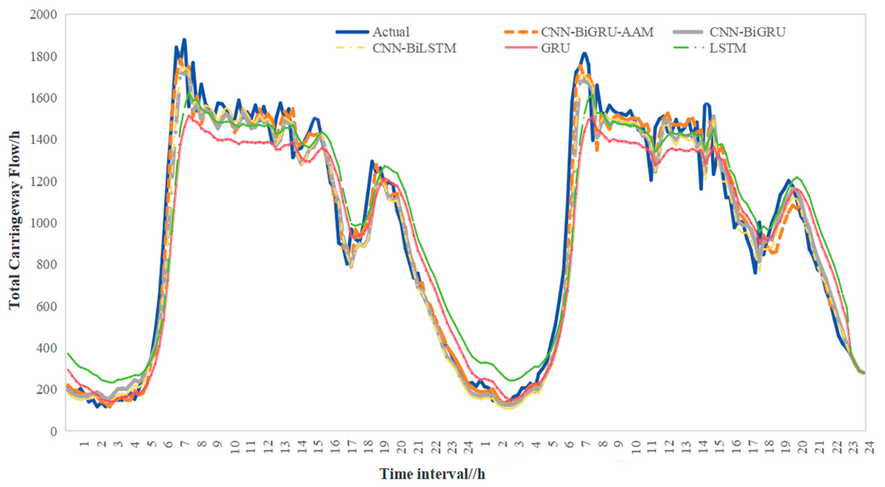
First, by integrating the driving conditions of vehicles on highways, the CNN-BiGRU-AAM model was validated for traffic flow prediction performance under different weather conditions and air quality levels. The results demonstrate that this model effectively captures the periodic nature of traffic flow and the characteristics of morning and evening peaks. Although the model’s predictive performance may be slightly affected in extreme weather conditions, its overall performance remains good, making it suitable for various scenarios in short-term traffic flow prediction.
(2)
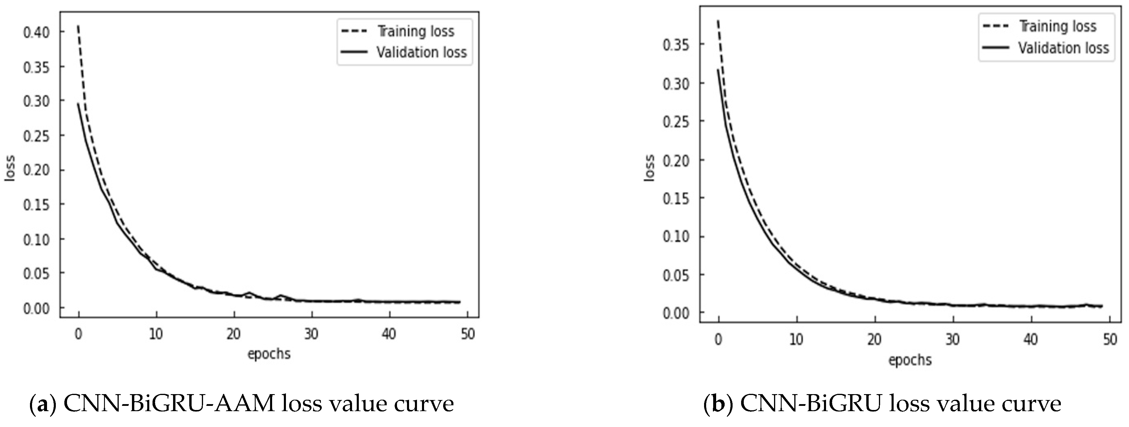
Additionally, regarding the spatiotemporal characteristics of traffic flow, the model was integrated and optimized; by concatenating the CNN and BiGRU into a multi-layer feature extraction model, it is possible to better analyze complex data. The CNN captures spatial features, while the BiGRU, by incorporating historical and future information, captures the long-term dependencies in time series data. Moreover, by utilizing isolation forests before data standardization, the model can effectively handle data missingness and anomalies, thereby improving its robustness.
(3)
Furthermore, the adoption of an additive attention mechanism enables the model to selectively prioritize important time steps and salient features through learnable linear mappings. Compared to traditional attention mechanisms, this dynamic mechanism enhances overall performance, resulting in improved predictive accuracy of the CNN-BiGRU-AAM model over benchmark models.
(4)
Finally, while integrating multiple models and techniques increases model complexity, requiring more computational resources and time for training and finetuning, future research will continue to optimize these aspects and explore additional factors that may affect traffic flow prediction performance. This will additionally boost the precision and versatility of the model, fulfilling the requirements for real-world traffic prediction.

Author Contributions

Conceptualization, S.L. and W.L.; methodology, W.L.; software, Y.W.; validation, Y.W., Y.W. and W.L.; formal analysis, S.L.; investigation, W.L.; resources, S.L.; data curation, W.L. and S.L.; writing—original draft preparation, W.L.; writing—review and editing, Y.P. and D.Z.Y.; visualization, Y.P.; supervision, D.Z.Y.; project administration, X.M.; funding acquisition, S.L. All authors have read and agreed to the published version of the manuscript.

Funding

This research was funded by the Chongqing Municipal Science and Technology Bureau Doctor Through Train Project (Grant No. CSTB2022BSXM-JCX0099) and the Team Building Project for Graduate Tutors in Chongqing (Grant No. JDDSTD2022004). This project was supported by the Open Fund of the Chongqing Key Laboratory of Traffic Systems and Safety in Mountain Cities (Chongqing Jiaotong University) (Grant No. 2018TSSMC04).

Institutional Review Board Statement

Not applicable.

Informed Consent Statement

Not applicable.

Data Availability Statement

Traffic flow data supports the findings of this study. Please send an email to [email protected] to obtain the data and discuss further.

Conflicts of Interest

The authors declare no conflicts of interest.

References

  1. Williams, B.M.; Durvasula, P.K. Urban freeway traffic flow prediction: Application of seasonal autoregressive integrated moving average and exponential smoothing models. Trans Res. Rec. 1998, 1644, 132–141. [Google Scholar] [CrossRef]
  2. Rojas, I.; Valenzuela, O.; Rojas, F.; Guillén, A.; Herrera, L.J.; Pomares, H. Soft-computing techniques and ARMA model for time series prediction. Neurocomputing 2008, 71, 519–537. [Google Scholar] [CrossRef]
  3. Kumar, S.V.; Vanajakshi, L. Short-term traffic flow prediction using seasonal ARIMA model with limited input data. Eur. Transp. Res. Rev. 2015, 7, 21. [Google Scholar] [CrossRef]
  4. Zhou, T.; Jiang, D.; Lin, Z.; Han, G.; Xu, X.; Qin, J. Hybrid dual Kalman filtering model for short-term traffic flow forecasting. IET Intell. Transp. Syst. 2019, 13, 1023–1032. [Google Scholar] [CrossRef]
  5. Kim, J.; Hwang, M.; Jeong, D.H.; Jung, H. Technology trends analysis and forecasting application based on decision tree and statistical feature analysis. Expert. Syst. Appl. 2012, 39, 12618–12625. [Google Scholar] [CrossRef]
  6. Aljahdali, S.; Hussain, S.N. Comparative prediction performance with support vector machine and random forest classification techniques. Int. J. Comput. Appl. 2013, 69, 12–16. [Google Scholar] [CrossRef]
  7. John, F.; Kolen; Stefan, C.; Kremer. Gradient Flow in Recurrent Nets: The Difficulty of Learning Long-Term Dependencies. In A Field Guide to Dynamical Recurrent Networks; IEEE: Piscataway, NJ, USA, 2001; pp. 237–243. [Google Scholar] [CrossRef]
  8. Zhang, W.B.; Yu, Y.H.; Qi, Y.; Shu, F.; Wang, Y.H. Short-term traffic flow prediction based on spatio-temporal analysis and CNN deep learning. Transp. A 2019, 15, 1688–1711. [Google Scholar] [CrossRef]
  9. Hochreiter, S.; Schmidhuber, J. Long Short-Term Memory. Neural Comput. 1997, 9, 1735–1780. [Google Scholar] [CrossRef]
  10. Cho, K.; Van Merriënboer, B.; Gulcehre, C.; Bahdanau, D.; Bougares, F.; Schwenk, H.; Bengio, Y. Learning phrase representations using RNN encoder-decoder for statistical machine translation. arXiv 2014, arXiv:1406.1078. [Google Scholar] [CrossRef]
  11. Hussain, B.; Afzal, M.K.; Ahmad, S.; Mostafa, A.M. Intelligent traffic flow prediction using optimized GRU model. IEEE Access 2021, 9, 100736–100746. [Google Scholar] [CrossRef]
  12. Dai, G.; Ma, C.; Xu, X. Short-term traffic flow prediction method for urban road sections based on space–time analysis and GRU. IEEE Access 2019, 7, 143025–143035. [Google Scholar] [CrossRef]
  13. Liu, S.; Peng, Y.; Shao, Y.M.; Song, Q.K. Highway Travel Time Prediction Based on Gated Recurrent Unit Neural Networks. Appl. Math. Mech. 2019, 40, 1289–1298. [Google Scholar] [CrossRef]
  14. Zhao, J.; Gao, Y.; Qu, Y.; Yin, H.; Liu, Y.; Sun, H. Travel time prediction: Based on gated recurrent unit method and data fusion. IEEE Access 2018, 6, 70463–70472. [Google Scholar] [CrossRef]
  15. Jeong, M.H.; Lee, T.Y.; Jeon, S.-B.; Youm, M. Highway Speed Prediction Using Gated Recurrent Unit Neural Networks. Appl. Sci. 2021, 11, 3059. [Google Scholar] [CrossRef]
  16. Reza, S.; Ferreira, M.C.; Machado, J.J.M.; Tavares, J.M.R.S. Traffic State Prediction Using One-Dimensional Convolution Neural Networks and Long Short-Term Memory. Appl. Sci. 2022, 12, 5149. [Google Scholar] [CrossRef]
  17. Lee, G.; Choo, S.; Choi, S.; Lee, H. Does the Inclusion of Spatio-Temporal Features Improve Bus Travel Time Predictions? A Deep Learning-Based Modelling Approach. Sustainability 2022, 14, 7431. [Google Scholar] [CrossRef]
  18. Narmadha, S.; Vijayakumar, V. Spatio-Temporal vehicle traffic flow prediction using multivariate CNN and LSTM model. Mater. Today Proc. 2023, 81, 826–833. [Google Scholar] [CrossRef]
  19. Ren, C.; Chai, C.; Yin, C.; Ji, H.; Cheng, X.; Gao, G.; Zhang, H. Short-Term Traffic Flow Prediction: A Method of Combined Deep Learnings. J. Adv. Transp. 2021, 2021, .1–15. [Google Scholar] [CrossRef]
  20. Yang, Y.Q.; Lin, J.; Zheng, Y.B. Short-Time Traffic Forecasting in Tourist Service Areas Based on a CNN and GRU Neural Network. Appl. Sci. 2022, 12, 9114. [Google Scholar] [CrossRef]
  21. Yuan, L.; Zeng, Y.; Chen, H.; Jin, J. Terminal Traffic Situation Prediction Model under the Influence of Weather Based on Deep Learning Approaches. Aerospace 2022, 9, 580. [Google Scholar] [CrossRef]
  22. Wang, B.W.; Wang, J.S.; Wang, T.Y.; Xia, T.Y.; Zhao, D.T. Multivariable traffic flow prediction model based on convolutional neural network and gate recurrent unit. JCQU 2023, 46, 132–140. [Google Scholar] [CrossRef]
  23. Schuster, M.; Paliwal, K.K. Bidirectional recurrent neural networks. IEEE Trans. Signal Process. 1997, 45, 2673–2681. [Google Scholar] [CrossRef]
  24. Zhao, S.; Zhao, Q.; Bai, Y.; Li, S. A Traffic Flow Prediction Method Based on Road Crossing Vector Coding and a Bidirectional Recursive Neural Network. Electronics 2019, 8, 1006. [Google Scholar] [CrossRef]
  25. Zhuang, W.; Cao, Y. Short-Term Traffic Flow Prediction Based on CNN-BILSTM with Multicomponent Information. Appl. Sci. 2022, 12, 8714. [Google Scholar] [CrossRef]
  26. Wang, S.; Shao, C.; Zhang, J.; Zhen, Y.; Meng, M. Traffic flow prediction using bi-directional gated recurrent unit method. Urban Inform. 2022, 1, 16. [Google Scholar] [CrossRef]
  27. Ma, C.; Zhao, Y.; Dai, G.; Xu, X.; Wong, S.C. A novel STFSA-CNN-GRU hybrid model for short-term traffic speed prediction. IEEE Trans. Intell. Transp. Syst. 2022, 24, 3728–3737. [Google Scholar] [CrossRef]
  28. Qu, D.; Wang, S.; Liu, H.; Meng, Y. A Car-Following Model Based on Trajectory Data for Connected and Automated Vehicles to Predict Trajectory of Human-Driven Vehicles. Sustainability 2022, 14, 7045. [Google Scholar] [CrossRef]
  29. Zhou, G.Z.; Guo, Z.; Sun, S.; Jin, Q.S. A CNN-BiGRU-AM neural network for AI applications in shale oil production prediction. Appl. Energy 2023, 344, 121249. [Google Scholar] [CrossRef]
  30. Zhang, X.J.; Zhang, G.N.; Zhang, H.; Zhang, X.L. Short-term traffic flow prediction based on ACBiGRU model. Huazhong Keji Daxue Xuebao 2023, 51, 88–93. [Google Scholar] [CrossRef]
  31. Chughtai, J.-u.-R.; Haq, I.u.; Islam, S.u.; Gani, A. A Heterogeneous Ensemble Approach for Travel Time Prediction Using Hybridized Feature Spaces and Support Vector Regression. Sensors 2022, 22, 9735. [Google Scholar] [CrossRef]
  32. Kiranyaz, S.; Avci, O.; Abdeljaber, O.; Ince, T.; Gabbouj, M.; Inman, D.J. 1D convolutional neural networks and applications: A survey. Mech. Syst. Signal Process. 2021, 151, 107398. [Google Scholar] [CrossRef]
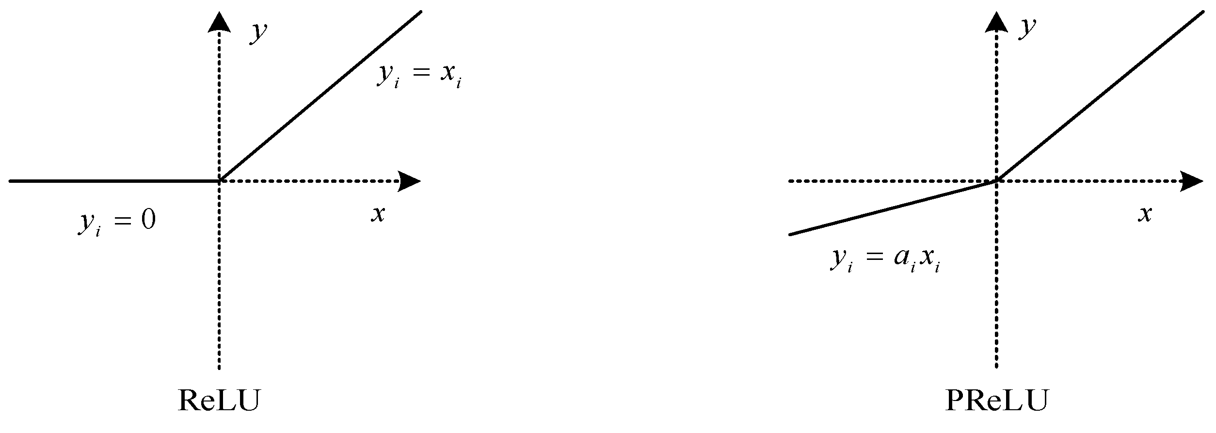
  33. Wei, Q.J.; Wang, W.B. Research on image retrieval using deep convolutional neural network combining L1 regularization and PRelu activation function. IOP Sci. 2017, 69, 012156. [Google Scholar] [CrossRef]
  34. Bahdanau, D.; Cho, K.; Bengio, Y. Neural machine translation by jointly learning to align and translate. arXiv 2014, arXiv:1409.0473. [Google Scholar] [CrossRef]
  35. Shen, T.; Zhou, T.; Long, G.; Jiang, J.; Pan, S.; Zhang, C. DiSAN: Directional Self-Attention Network for RNN/CNN-Free Language Understanding. arXiv 2017, arXiv:1709.04696. [Google Scholar] [CrossRef]
  36. Kingma, D.P.; Ba, J. Adam: A method for stochastic optimization. arXiv 2014, arXiv:1412.6980. [Google Scholar] [CrossRef]
Figure 1. Internal architecture of GRU.
Sustainability 16 01986 g001
Figure 2. Structure of the Bi-GRU network.
Sustainability 16 01986 g002
Figure 3. Hybrid deep neural network.
Sustainability 16 01986 g003
Figure 4. Correlation heatmap.
Sustainability 16 01986 g004
Figure 5. Comparison of Relu and PRelu functions.
Sustainability 16 01986 g005
Figure 6. Comparison of predictions from different models.
Sustainability 16 01986 g006
Figure 7. Comparison of predictions for different model “test sets”.
Sustainability 16 01986 g007
Figure 8. Combinatorial model loss value curve.
Sustainability 16 01986 g008
Table 1. Model parameter constraints.
LayerAttributionParameterValue
1CNNConv1D-1 neurons128
Conv1D-2 neurons64
2Bi-GRUneurons16
Dropout0.2
recurrent_regularizer0.01
3Denseneuron1
Table 2. Model training set error indicator values.
Predictive ModelPerformance Indicators
Training RMSETraining MAETraining MAPE Training   R 2
CNN-BiGRU-AAM97.0169.019.85%0.96
CNN-BiGRU121.2182.4311.68%0.94
CNN-BiLSTM123.3684.1511.54%0.93
GRU154.48107.9414.99%0.90
LSTM153.48115.3119.09%0.90
Table 3. Model test set error indicator values.
Predictive ModelPerformance Indicators
Test RMSETest MAETest MAPE Test   R 2
CNN-BiGRU-AAM96.4667.148.77%0.97
CNN-BiGRU109.8174.909.93%0.96
CNN-BiLSTM108.8974.079.99%0.96
GRU143.9597.8614.04%0.92
LSTM145.69110.1019.51%0.92
Table 4. ANOVA results table.
ANOVA a
ModelSum of SquaresDegrees of FreedomMean SquareFSignificance
Regression195,900,654.9351195,900,654.93521,849.620<0.001 b
Residual7,728,572.1598628965.861
Total203,629,227.094863
a. Dependent variable: CNN-BiGRU-AAM; b. predictors: (constant), true.
Disclaimer/Publisher’s Note: The statements, opinions and data contained in all publications are solely those of the individual author(s) and contributor(s) and not of MDPI and/or the editor(s). MDPI and/or the editor(s) disclaim responsibility for any injury to people or property resulting from any ideas, methods, instructions or products referred to in the content.

