Quantifying Sectoral Carbon Footprints in Türkiye’s Largest Metropolitan Cities: A Monte Carlo Simulation Approach

Abstract

Urbanization is a substantial contributor to greenhouse gas (GHG) emissions, a pivotal factor in climate change. Climate change represents a global predicament impacting all nations, necessitating collaboration among numerous countries to curtail GHG emissions. An essential step to overcome this problem is the accurate measurement, calculation, and modelling of the amount of damage inflicted on the atmosphere. Therefore, carbon footprints (CFs) originating from various sources are calculated. This study calculates the CF of different sectors in metropolitan cities in Türkiye, which are Istanbul, Ankara, and Izmir, for the years 2015–2020 using the Tier 1 and Tier 2 approaches outlined in the Intergovernmental Panel on Climate Change (IPCC) methodology. Additionally, to account for uncertainties in activity data and emission factors and calculate the potential emission range, a Monte Carlo simulation (MCS) was conducted. Analysis of Tier 1 results revealed the highest emissions consistently occurring in Istanbul across all years, while emissions from other cities exhibited variability annually. Notably, average MCS results surpassed the total emission quantities derived at the study’s conclusion for all cities and years, underscoring the influence of uncertainties. The study results align with the calculated 95% confidence interval, affirming the robustness within the specified statistical framework.

1. Introduction

Climate change is an incontrovertible challenge of our era, with far-reaching implications for the planet’s ecological balance and human societies [1,2,3,4]. Urbanization is often identified as a significant contributor to greenhouse gas (GHG) emissions, which are a major cause of climate change [5,6,7,8]. Experts predict that by 2050, cities, which already house half of the global population, will be home to seven out of every ten people in the world [9,10,11]. This rapid growth of urban populations, particularly in Asia and Africa [7,12], is a significant factor in the increasing levels of GHG emissions and the resultant climate change. Urbanization has historically underpinned economic growth, transforming cities into hubs of industry, commerce, and innovation [10,13]. This shift has led to significant changes in energy consumption patterns, as populations transition from less energy-intensive agricultural activities to highly energy-consuming service and industrial sectors [7,14,15]. In parallel, experts predict that by 2030, cities will account for a staggering 73% of the world’s energy consumption, underscoring the urgent need for sustainable, low-carbon energy solutions [16].

Since the past, most of our energy needs have been met with fossil fuels, resulting in a steep environmental cost [7,17,18,19]. Fossil fuels are major contributors to the increase in atmospheric carbon dioxide (CO₂) levels [20,21,22,23], which have risen from 270 ± 20 ppm in the pre-industrial era [24,25] to over 400 ppm today, a 150% increase [26]. The report from the Intergovernmental Panel on Climate Change (IPCC) notes that while 62% of global emissions were generated from urban areas in 2015, this value has risen to 67–72% in 2020 [27]. Urban GHGs include both direct emissions of fossil fuels used to generate energy in various sectors, such as industry, transportation, and buildings [28], as well as indirect emissions of resources such as electricity, water, food, and gasoline that are not produced within city limits [29]. All these processes return to nature as primary and secondary carbon footprints (CFs), respectively [30,31]. CF is a relatively new concept that has gained attention in the literature over the last decade [32]. CF, which is expressed in many ways in the literature, can be defined as the CO₂ equivalent (CO₂e) expression of direct or indirect anthropogenic activities or the GHGs produced during the entire lifetime of a product [5,23,31,33,34,35,36,37]. This concept can be calculated at different scales, from international to urban levels, using various methods and boundaries [38]. Calculating CFs is instrumental in bridging consumer behavior, emissions, and policy makers [33]. However, the complexity of CF calculations presents challenges [38,39]. These complexities arise from terminological variations [40,41], choices regarding which gases to include, boundary definitions, city typologies, methodological approaches [42,43,44,45], and the metrics employed to express them [46].

Several studies and protocols have been conducted to consolidate emission inventories in urban areas [47,48,49,50,51]. However, despite the presence of multiple standards and protocols, the calculation of CFs for cities is often more intricate than estimating national emissions. This complexity stems from the unique challenges associated with accounting for diverse emission sources, evaluating their impact at the city level, and establishing appropriate boundaries and measurement/reporting methodologies [42,51,52,53,54]. Considering the potential divergence in results stemming from the use of different methodologies, it is crucial to take into account a specific approach when comparing CFs across cities or regions.

Türkiye, like many nations, faces the consequences of urbanization driven by industrial development, tourism, and educational opportunities, especially in cities such as Ankara, Istanbul, and Izmir [55]. This urbanization, parallel with a population exceeding 84 million [56] and burgeoning economic activity, has led to a six-and-a-half-fold increase in energy consumption compared to fifty years ago [57], catapulting Türkiye to fifteenth place in the global energy consumption rankings [58]. While efforts to boost renewable energy have been made, fossil fuels still dominate the energy landscape, making Türkiye a significant global GHG emitter [59,60,61,62]. In 2021, Türkiye ranked thirteenth globally in GHG emissions [63], releasing 564.4 MtCO₂e into the atmosphere. There has also been an increase in per capita emissions, with the emission rate per person increasing from 4 tons (t) CO₂e person⁻¹ in 1990 to 6.7 tCO₂e person⁻¹ in 2021 [64]. As part of the 27th Conference of the Parties (COP27), Türkiye has declared in its Nationally Determined Contribution that it will reduce GHG emissions by 41% by 2030 compared to the reference scenario and reach peak emissions in 2038. Additionally, Türkiye has set a net-zero emissions target by 2053 [65]. In addition to national emission inventory studies, Türkiye, which places importance on the efforts of local governments in combating climate change, is a signatory to the Global Covenant of Mayors for Climate and Energy (GCoM) with 50 local administrations. The aim is to reduce emissions, enhance local climate resilience, and achieve clean energy access through collaboration with other participating local governments [66]. Additionally, Istanbul, as a member of the C40 network, aims to halve its emissions within 10 years, increase equity in addressing climate change, and strengthen resilience [67].

As a result, since cities are the focal point of future mitigation and adaptation efforts, it is of great importance to regularly update the inventories of cities [68]. One of the most significant features that make this study valuable on both a global and local scale is the acquired data. This is because the fundamental challenges in creating GHG emission inventories at the city level is the lack of existing data. In this study, conducted for the provinces of Ankara, Istanbul, and Izmir, data were obtained from various official and private institutions, official documents, internet sources, and personal interviews. These cities are the most densely populated cities in Türkiye and hold prominent positions on the global scale, with respective rankings of 15th, 77th, and 157th [69]. Therefore, GHG emissions play a significant role. Additionally, the membership of these cities in GcOM and C40 places extra emission-decreasing responsibilities on them. Therefore, in this study, these cities have been chosen as the areas of interest. Furthermore, when examining the literature, it is observed that CF calculations are generally not based on real data; instead, consumption data are obtained through various modeling results, and CFs are calculated based on these model outcomes. The situation is similar for cities in Türkiye, and this study was conducted due to the absence of a comparative CF calculation based on realand long-term data. In this study, data were sequentially collected for various sectors, emission factors (EFs) were determined for the IPCC’s Tier 1 and Tier 2 approaches, and then CF calculations were performed. The calculation conducted for the years 2015–2020 resulted in the comparison of both the changes in emissions within cities over the years and the relative positions of the cities. Subsequently, using the Monte Carlo simulation (MCS) approach, an uncertainty analysis of emissions for these three major cities was presented.

The primary objective of this paper is to offer guidance to researchers engaged in city-specific CF studies and to provide preliminary insights for policymakers, aiding them in attaining low carbon emission targets through established methodologies utilizing measured data. Additionally, another objective is to mitigate uncertainties in CF sectors associated with data deficiencies by implementing the MCS methodology across all considered metropolitan centers, intending to instigate a discussion with real-world examples. Through these approaches, the applied methodology is poised to serve as a valuable and reliable reference for technicians, meteorologists, climate scientists, and environmental professionals.

The rest of this paper is organized as follows. Section 2 presents a literature review on CFs. Section 3 includes material and methods and study area. Section 4 gives the results and discussion. Section 5 concludes the paper.

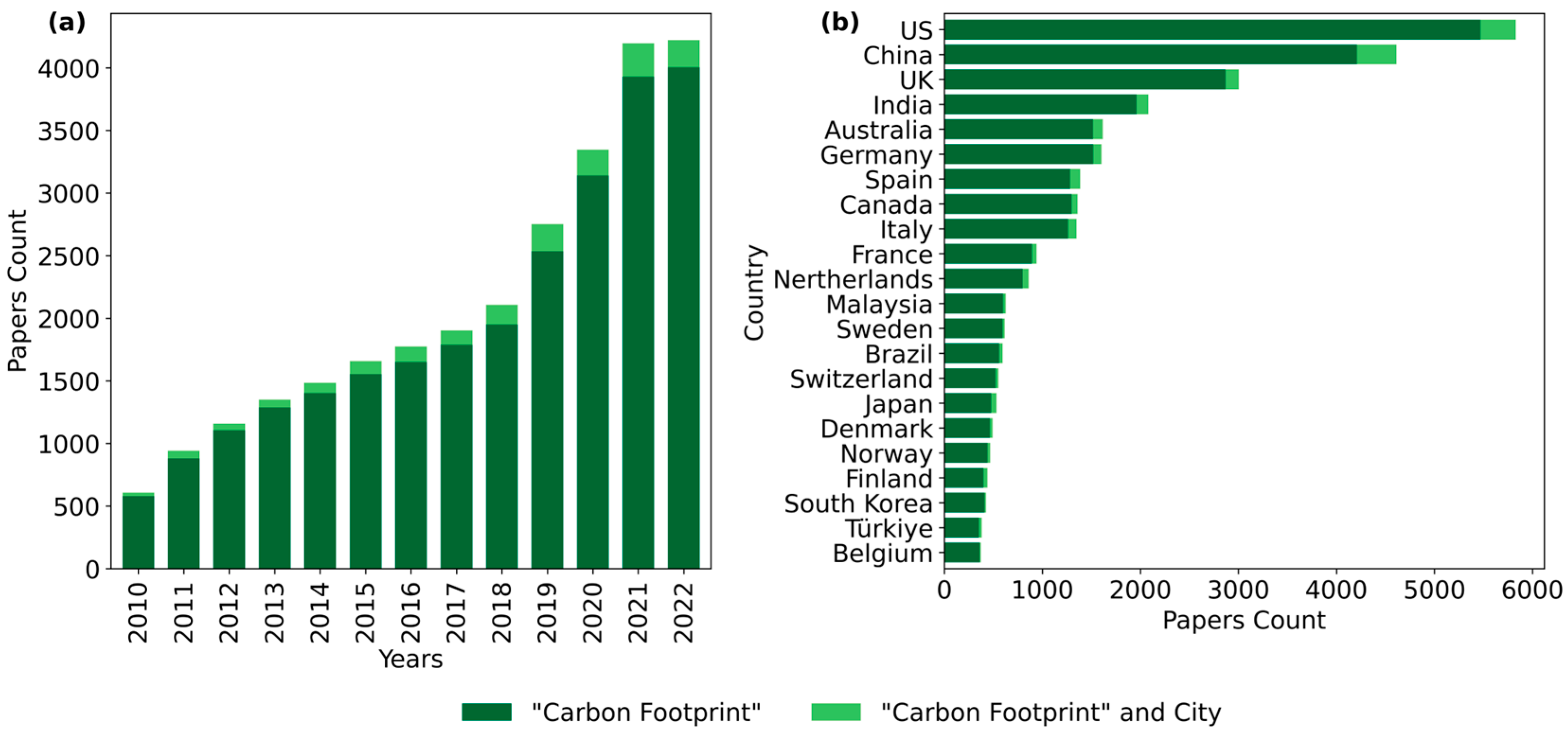
2. Literature Review on Carbon Footprint

The concept of CF has gained significant attention in academic research over the past decade, with numerous studies published on the topic at both national [13,36,70,71,72,73,74,75,76,77,78,79,80] and city scales [5,17,37,40,43,44,81,82,83,84,85,86,87,88,89]. Figure 1a shows the results of a ‘CF’ search conducted in the SCOPUS database, which returned a total of 25,809 articles that included the term in their article title, abstract, or keywords from 2010 to 2022. When the search was narrowed to include the terms ‘CF’ and ‘City’, it resulted in 1699 articles [90]. It appears that, as shown in Figure 1b, the United States (US) has conducted the most studies on ‘CF’ as a topic, followed by China. In contrast, when it comes to studies specifically focused on ‘CF’ and ‘City’, the trend is reversed, with China leading the way and the US following. This suggests that CF analyses conducted at the city scale are relatively limited in comparison to those at the national scale. In Türkiye, there have been relatively few studies on CF compared to other countries. Since 2010, there have been 352 studies conducted on the subject of ‘CF’, and only 29 of these are related to cities.

Although cities are commonly perceived as the primary source of GHG emissions, numerous studies in the literature indicate that urbanization has an overall mitigating effect on total emissions. Additionally, there is evidence suggesting that urban households exhibit lower direct emissions compared to rural households [91]. In parallel, a study based in Germany has determined that rural areas produce 11% more emissions compared to urban areas. It has been observed that shorter distances in cities, along with the use of public transportation and smaller apartment sizes, result in a 35% reduction in direct emissions. Due to income disparities, particularly in the Rhine and Ruhr regions, higher emissions have been noted in rural areas [92]. Similarly, in some Western European countries such as the United Kingdom, France, and Belgium, high rural emissions have been observed [93,94], and also, in a study conducted in the US, it has been asserted that metropolitan areas are more carbon-efficient compared to smaller or rural settlements [95]. Additionally, Dodman [5] and Argun et al. [96] found that cities outside Shanghai and Beijing and the Konya Selçuklu district, respectively, exhibit significantly lower per capita CO₂e emissions compared to their respective countries. Singh and Kennedy [97] have indicated that a 2% decrease in urban density could lead to a 346% and 428% increase in emissions from electricity and transportation, respectively, by 2050. Additionally, Rybski et al. [98] have concluded that urbanization triggers climate change in developing countries while mitigating climate change in developed ones.

On the other hand, according to Wiedmann et al. [99], cities are associated with approximately 70–80% of global CO₂ emissions because they are accountable for emissions not only within their own boundaries but also arising from the import of goods and services. Neglecting goods and services’ emissions in the five major cities responsible for over half of Australia’s national CF would result in underestimating the national CF by a quarter [100]. When considering a more comprehensive life cycle analysis of urban emissions, it is believed that cities actually contribute to emissions that are 7% to 24% higher in reality [101]. With the increasing urbanization of Eastern Europe, CF has evidently risen there [102]. Similarly, in the urbanization process of Beijing, there has been an observed increase in total household energy consumption from 22.7% to 59.2%, and the overall household CO₂ emission rate has risen from 32.2% to 68.8% [103]. The per capita average CF in urban areas tends to be two to nine times higher compared to those of residents living in rural areas [104]. In parallel, the results of survey data on consumption across various sectors in Mumbai revealed that the per capita annual average CF in urban areas is 2.5 tCO₂e, compared to 0.85 tCO₂e in rural areas [105], and a study encompassing 252 cities indicated an average per capita CF of 5.31 tCO₂ in urban areas and 3.41 tCO₂ in rural areas [38]. In a manner akin to these studies, an examination of 434 municipalities in the United Kingdom consistently showed a larger CF in urban areas based on the average findings of the study [81].

Globally, emissions in urban areas are dense due to population, income, and consumption excess [86]. In intricate detail, it has been understood that per capita GHG emissions in cities of developed countries surpass those in cities of developing nations, with cities in Asia having the highest overall emissions [106]. In the world, while cities located in developed countries, such as Seoul, Guangzhou, and New York, take the lead in emission rankings [86], the city of Melbourne in Australia has been noted for its total CF reaching 100 MtCO₂e, with a per capita value of 25.1 tCO₂e [99]. Hachaichi and Baouni [38] have emphasized that, similar to developed cities, CF is significant in developing cities, highlighting the importance for local authorities to pay attention to these emissions. In parallel to these findings, Bozdağ [107] has stated that Istanbul, Ankara, Izmir, and Antalya, with their high populations, income levels, metropolitan identities, and presence of capital and industrial sectors, have had the highest carbon emissions since 2014; Burdur was noted to have a per capita CO₂ emission of 3.62 t yr⁻¹, exceeding the Turkish average, marking it as a developing city that warrants attention in terms of carbon emissions [108].

3. Material and Methods

3.1. Study Areas

This study entails a CF analysis for three prominent metropolitan cities in Türkiye, namely Ankara, Istanbul, and Izmir. These cities were selected due to their population exceeding four million people in 2022, rendering them the most populous and developed urban areas in the country. The land use in the study areas were geographically represented using QGIS (Figure 2).

Ankara: Ankara is a city of significant political and economic importance in Türkiye, serving as the country’s capital. It is situated in the Central Anatolia region (39°55′ N and 32°51′ E), which is known for its agricultural productivity and strategic location. The city covers an area of around 26 thousand km² and has a population of approximately 5.8 million people as of 2023, making it the second most populous city in the country. In terms of economic output, Ankara ranked second in Türkiye in 2021 with a gross domestic product (GDP) of 35.1 billion dollars. Over the years, the city has transitioned from an agricultural economy to one dominated by trade and industry, with eleven organized industrial zones and a particular focus on the defense industry [109]. In the southern portion of Ankara, a steppe climate is observed, while in the northern, the mild and rainy variations of the Black Sea climate can be seen. This region is dominated by a continental climate; winter temperatures are low, while summers are hot [110].

Istanbul: Istanbul, located in the Marmara Region (41.01° N and 28.95° E) of Türkiye, is a city with a rich history and culture. The city has a surface area of 5461 km² and is the most populous city in Türkiye. Its population has been steadily growing and has reached 15,907,951 as of 2023. In addition to its cultural and historical significance, Istanbul is the industrial and production hub of Türkiye and plays a significant role in the country’s economy. In fact, in 2021, it reached the highest GDP among all cities in Türkiye at $115.9 billion [111]. Istanbul’s climate is classified as a Mediterranean climate according to the Köppen climate classification. The city experiences mild winters and very hot summers [110]. Due to its location and geography, Istanbul is also prone to natural disasters such as earthquakes and floods.

Izmir: Izmir is a coastal city located in the western part (38.4° N and 27.17° E) of Türkiye. Izmir is the third most populous city in Türkiye with a population of 4,462,056 people as of 2023 and a land area of 11,891 km². The city’s economy is based on various sectors such as service, industry and agriculture, which has contributed to its GDP of $24.3 billion in 2021, ranking third among Türkiye’s major metropolitan cities. Izmir is also renowned for its tourism industry, as it attracts many visitors with its historical and natural attractions [112]. The city has a Mediterranean climate, with warm winters, very hot summers, and arid weather, according to the Köppen climate classification system [110].

3.2. Emissions Inventory Method

When conducting an analysis of a city’s CF, various methods can be employed for inventory and calculation purposes. In this study, the researchers chose to utilize the IPCC methodology. This method serves as a common foundation for other standards and protocols and is frequently employed as the primary approach for developing a city-scale emission inventory. To establish a city-scale emission inventory using the IPCC methodology, direct GHG emissions, including CO₂, methane (CH₄), and nitrous oxide (N₂O), were calculated for the stationary, mobile combustion, enteric fermentation, solid waste disposal (SWD), and composting sectors annually from 2015 to 2020. Subsequently, the emissions from each sector were multiplied by their respective global warming potentials (28 for CH₄, 265 for N₂O) and converted to the CO₂e unit, which is a standard unit used to compare GHG emissions of different gases. In the estimation of GHG emissions for the study, the researchers employed the methodologies described in Tiers 1 and 2, as suggested by the IPCC, given the unavailability of Tier 3 data [113]. Additionally, the study incorporated data on the amount of carbon stored by cities based on forest management plan data. Finally, utilizing MCS, the potential ranges of emissions in three different cities have been delineated. Subsequent to the meticulous completion of computational processes, a comprehensive and systematic analysis unfolded, wherein detailed comparisons were executed among distinct cities, taking into account the specific years that were included in the overarching analytical framework.

3.3. Greenhouse Gas Emission from the Energy Sector

The energy sector plays a pivotal role in GHG emissions [114], encompassing both stationary and mobile combustion sources. Combustion processes in this sector release a substantial amount of carbon, primarily in the form of CO₂. Developed countries attribute a significant portion of GHG emissions to the energy sector, with 90% of CO₂ emissions and 75% of total GHG emissions originating from this sector [113]. Similarly, in Türkiye, the energy sector contributes significantly to CO₂ emissions, with 85.4% of total emissions in 2020 coming from this sector [64]. Equation (1) in

Table 1. Equations used for GHG emission from the energy sector [113,115,116].

Equation	Explanation of Parameters in Equation	Equation Number
$Emissio{n}_{GHG,fuel}={FC}_{fuel}\times {NCV}_{fuel}\times E{F}_{GHG,fuel}\times {10}^{-3}$	$Emissio{n}_{GHG,fuel}$ is the total amount of emissions according to fuel and GHG (t), ${FC}_{fuel}$ is the amount of fuel burned (t), ${NCV}_{fuel}$ is the fuel’s net calorific value (TJ kt−1), $E{F}_{GHG,fuel}$ is the assumed EF of GHGs according to fuel type (t GHG TJ−1)	(1)
$T{otal emissions}_{heat}=\frac{\left(HO/{Eff}_O\right)}{\left(\left(HO/{Eff}_H\right)+\left(EO/{Eff}_E\right)\right)}$	$HO$ is the heat output, $EO$ is the electricity output, ${Eff}_O$ is the total efficiency of output, ${Eff}_H$ is the efficiency of heat plant,${Eff}_E$ is the efficiency of electricity plant	(2)
$Total FC=NV\times D\times FC\times FD\times {10}^{-6}$	$Total FC$ is the fuel consumed (FC) amount for different fuels (kt), $NV$ is the number of vehicles, $D$ is the traveled by different vehicle types (km).$FC$ represents the amount of FC per 100 km (L 100km−1), and $FD$ is the density values of different fuels (kg L−1)	(3)
$Emission={\sum }_{a,b,c}\left[{FC}_{a,b,c}\times F_{a,b,c}\right]$	As subscript consideration ‘$a$’, ‘$b$’, ‘$c$’ represents the type of fuel used by the vehicle, type of vehicle, the emission control technology, respectively	(4)
${VR}_{a,b}=\frac{{NV}_{a, b}}{N{V}_{total}}$	${VR}_{a,b}$ expresses the ratio of the number of vehicles to the total number of vehicles according to vehicle and fuel type	(5)
$Total FC=\sum _{a,b}\left[{VR}_{a,b}\times {WT}_{a,b}\times FC\times FD\times {10}^{-6}\right]$	${WT}_{a,b}$ expresses the way traveled with different vehicle and fuel types in one year (vehicle-km)	(6)
$Total Emissions= LTO Emissions+Cruise$	$LTO Emissions$ is the emission amount at landing and landing/taking off cycle (LTO), $Cruise$ is the emission amount at cruise	(7)
$LTO Emissions=Number of LTOs +{EF}_{LTO}$	${EF}_{LTO}$ is the EF belonging to LTO	(8)
${LTO}_{FC}=Number of LTOs+FC per LTO$	${LTO}_{FC}$ is the FC at LTO	(9)
$Cruise Emissions=\left({Total}_{FC}-{LTO}_{FC}\right)\times {EF}_{Cruise}$	${Total}_{FC}$ is the FC at LTO and cruise, ${EF}_{Cruise}$ is the EF belonging to cruise	(10)
$FC in City=FC in Country\times \left(\frac{PNC}{PNCO }+\frac{FNC}{FNCO}\right)/2$	$PNC$ and $PNCO$ are the number of passengers transported within the city and country, respectively. $FNC$ and $FNCO$ are the amount of cargo transported within the city and country, respectively	(11)
$FC in City=FC in Country\times \left(\frac{RLC}{RLCO}\right)$	$RLC$ and $RLCO$ expresses the length of non-electrified railway in the city and country (km).	(12)

is employed to estimate emissions from the energy sector using Tier 1 and Tier 2 approaches.

Table 2. NCV (TJ kt⁻¹) and CO₂ EF (kg TJ⁻¹) of different fuels [113].

Fuel Type	Gasoline (Engine, Aviation, Jet)	Diesel	Fuel Oil	Natural Gas	Liquefied Petroleum Gas (LPG)	Jet Kerosene	Anthracite
NCV	44.3	43	40.4	48	47.3	44.1	26.7
EF	69,300–70,000	74,100	77,400	56,100	63,100	71,500	98,300

displays the net calorific values (NCVs) and CO₂ EFs used in Tier 1 for different types of fuels.

Table 3. Türkiye-specific CO₂ EFs (kg TJ⁻¹) for different fuels [64].

Fuel Type	2020	2019	2018	2017	2016	2015
Diesel	72,280	72,280	72,280	72,280	73,430	73,430
Natural gas	53,670	53,670	55,250	55,620	56,060	55,090
Coal	98,100	98,100	99,430	98,080	96,650	99,270

presents country-specific CO₂ EFs utilized in the Tier 2 method for estimating GHG emissions from the energy sector. However, for CH₄ and N₂O emissions, there are no specific EFs available for Türkiye. Therefore, the EFs recommended by the IPCC should be applied in the calculations of these GHG emissions for Türkiye.

3.3.1. Greenhouse Gas Emissions from Stationary Combustion

The stationary combustion category typically accounts for approximately 70% of GHG emissions from the energy sector. Emissions from stationary combustion encompass a variety of sectors, such as energy industries, manufacturing industry and construction (In Figure 3, it is labeled ‘Man. Ind. & Const.’). These sectors commonly utilize diverse fuels, including natural gas, coal, electricity, and fuel oil. EFs from these sectors are provided in Tables S1 and S2 [113].

In addition to emissions from fuels, it is crucial to calculate GHG emissions arising from electricity consumption. Typically, these emissions are estimated based on country-specific electricity EFs. In Türkiye, only CO₂ EFs for electricity grid emissions have been officially reported for the years 2018–2020 by the Ministry of Energy and Natural Resources (MENR) [117]. However, for the sake of consistency in this study, all electricity EFs related to CO₂, CH₄, and N₂O of Türkiye given in

Table 4. Electricity grid EFs of Türkiye by year (kg kWh⁻¹).

Years	CO2	CH4	N2O	CO2e
2020	0.722469	0.00025	0.00416	0.72688
2019	0.793630	0.00025	0.00407	0.79795
2018	0.710062	0.00023	0.00420	0.71450
2017	0.676377	0.00024	0.00565	0.68227
2016	0.711725	0.00026	0.00580	0.71779
2015	0.689520	0.00026	0.00557	0.69535

have been computed using various assumptions (Equation (2), Table 1) as employed in Brander et al. [115].

3.3.2. Greenhouse Gas Emissions from Mobile Combustion

Greenhouse Gas Emissions from Road Transport

Within the category of road transportation, various vehicle types, including cars, light trucks, buses, and motorcycles, operate on different types of liquid and gaseous fuels. Two distinct methods are employed to estimate emissions from road transport. The Tier 1 method calculates emissions using the amount of FC. In Tier 2, emissions from road transport are estimated based on the distance vehicles travel. If datasets required for both Tier 1 and Tier 2 methods are available, it is crucial to make predictions and comparisons for both methods. EFs from road transportation are presented in Table S3 [113].

In the emission calculation using the Tier 2 approach, data on vehicle types, the specific fuel employed by each vehicle, and, when accessible, details on emission control technologies are incorporated. The total FC is then computed based on the distance covered by each vehicle, and subsequently, Equations (3) and (4) in Table 1 are employed to ascertain the emissions discharged into the atmosphere for each vehicle and fuel type.

In this study, European EFs from the guide were employed due to the resemblance between vehicles in Türkiye and Europe. While the utilization of Europe-based values for Türkiye introduces a degree of uncertainty into the results, the objective was to enhance comparability with the Tier 1 approach, given the assumptions made. Furthermore, owing to the absence of data regarding vehicle types on the road, no distinctions were made based on emission control technology [118,119]. Table S4 presents FC and EFs for various fuel types utilized in road transportation [120]. Additionally, vehicles traversing through a city but not registered in that city also contribute to GHG emissions in the considered city. To calculate these emissions from transit, the method outlined by Kocaeli Metropolitan Municipality (KMM) was employed, as detailed in Equations (5) and (6) in Table 1 [116].

Greenhouse Gas Emissions from Civil Aviation

GHG emissions from aviation stem from the combustion of jet fuel and aviation gasoline. Several factors influence these emissions, including the number and type of cruises, the types and efficiency of aircraft engines, flight times and flight levels, and LTO. The Tier 1 method is typically employed to calculate emissions from small airplanes and aviation gasoline consumption. However, if data on aircraft activities are unavailable, the Tier 1 method can also be used for jet fuels. In Tier 2, emissions depend on FC as well as aircraft types and LTO numbers by aircraft types. The calculations using Tier 1 and Tier 2 methods employed Equations (1) and (7)–(10) given in Table 1, respectively. The EFs utilized in the calculation of Tier 1 and Tier 2 emissions from civil aviation are provided in Tables S5 and S6 [113,120].

Greenhouse Gas Emissions from Railway Transport

Railway transportation encompasses three types of locomotives: electrical, diesel, and steam [121]. In this study, GHG emissions resulting exclusively from the combustion of diesel fuel were calculated. Since the FC amounts for railway transportation were unavailable at the provincial level, they were estimated using the approaches outlined in Equations (11) and (12), Table 1 [116]. Due to insufficient data on railway transportation, only the Tier 1 method was employed. The EFs for CH₄ and N₂O from fossil fuels used in railway transportation are detailed in Table S7 [113].

Greenhouse Gas Emissions from Water-Borne Transportation

The domain of water-borne transportation encompasses all forms of water transport, ranging from boats propelled by diesel engines, steam, or gas turbines to large cargo ships [122]. Typically, marine transportation employs three main types of fuel: fuel oil, diesel, and gasoline. Owing to a scarcity of data on maritime transport, exclusively the Tier 1 method has been applied in this study. The EFs for CH₄ and N₂O utilized in marine transportation are 7 and 2 kg TJ⁻¹, respectively [113].

3.4. Greenhouse Gas Emissions from Agriculture, Forestry and Other Land Use

GHG emissions and carbon storage on managed land are comprehensively delineated within the forest, agriculture, grassland, wetland, settlement, and other land categories in the agriculture, forestry, and other land use (AFOLU) sector. Within the scope of this study, calculations were exclusively conducted for CH₄ emissions originating from enteric fermentation within the agricultural sector and the quantification of carbon storage in forests. Access to additional data for other components was regrettably unavailable.

3.4.1. Methane Emission from Enteric Fermentation

CH₄ is generated as a by-product of carbohydrate digestion in the rumen of ruminant, non-ruminant, and monogastric animals that consume grass. Ruminants, among these animals, exhibit comparatively higher CH₄ emissions. The quantity of CH₄ emitted by animals and EFs are contingent on factors such as their age, weight, type, and quantity of feed. As per the IPCC, the CH₄ EFs for livestock, including cattle, horses, mules, asses, camels, sheep, pigs, and goats, in developing countries are 55, 18, 10, 46, 5, 1, and 5 kg CH₄ head yr⁻¹, respectively. For Türkiye, the EFs for cattle emissions are 60.98, 60.90, 60.62, 60.87, 60.72, and 60.96 kg CH₄ head yr⁻¹ for the years 2015–2020, respectively. Emissions from enteric fermentation are calculated using Equation (13).

$$Total C{H}_{4_{Enteric}}=\sum {EF}_{\left(T\right)}\times \left(\frac{N_{\left(T\right)}}{{10}^6}\right)$$

(13)

Here, ‘$Total C{H}_{4_{Enteric}}$’ represents the total CH₄ emissions from enteric fermentation, ‘${EF}_{\left(T\right)}$’ is the EF for the defined population of livestock, ‘$N_{\left(T\right)}$’ is the total number of livestock of each species within the country, and ‘$T$’ is the different livestock species [113].

3.4.2. Total Carbon Accumulation in Forest Land

In the IPCC, it is emphasized that each country should develop its own coefficients to achieve a more realistic approach to carbon accumulation in forest land [123]. In the study conducted by Tolunay, the biomass expansion factor (BEF) employed in the IPCC guidelines has been revised for Türkiye [124]. The carbon balance calculation method outlined in ‘Ecosystem-Based Functional Forest Management Plans Preparation Communiqué’ also utilizes equations for carbon calculations provided in

Table 5. Amount of carbon stored in forest land (t) [125].

Carbon Pool	Tree Type	Productive Forest	Degraded Forest
AGB	Coniferous	VO × D × BEF	VO× D × BEF
	Broadleaved	VO × D × BEF	VO× D × BEF
BGB	Coniferous	AGB × R	AGB × R
	Broadleaved	AGB × R	AGB × R
∆CAGB	Coniferous	AGB × CFB	AGB × CFB
	Broadleaved	AGB × CFB	AGB × CFB
∆CBGB	Coniferous	BGB × CFB	BGB × CFB
	Broadleaved	BGB × CFB	BGB × CFB
DWC	Coniferous	AGB × 0.01 × CFDW	AGB × 0.01 × CFDW
	Broadleaved	AGB × 0.01 × CFDW	AGB × 0.01 × CFDW
DLC	Coniferous	F1 × CDL	F3 × CDL
	Broadleaved	F2 × CDL	F4 × CDL
Organic carbon in soil	Coniferous	F1 × CS	F3 × CS
	Broadleaved	F2 × CS	F4 × CS
Total Carbon		∆CAGB + ∆CBGB + DWC + DLC + Organic carbon in soil

along with new coefficients (Table 6).

In this table, ‘AGB’ and ‘BGB’ refer to above-ground and below-ground biomass (t), respectively. ‘VO’ denotes total volume overbark (m³), and ‘D’ represents the basic wood density (t m⁻³) for each species or group of species. Carbon stocks in above-ground and below-ground biomass are denoted as ‘∆C_AGB’ and ‘∆C_BGB’ (t), respectively. ‘R’ is the conversion factor for calculating root biomass from above-ground biomass. ‘CF_B’ is the carbon conversion factor from biomass to carbon [126] and ‘CF_DW’ is the carbon conversion factor for dead wood biomass. ‘DWC’ and ‘DLC’ refer to the amount of carbon (t) in dead wood and dead litter, respectively. ‘F1’ and ‘F2’ represent coniferous and broadleaved areas in productive forests, while ‘F3’ and ‘F4’ signify coniferous and broadleaved areas in degraded forests, respectively. ‘CDL’ represents the amount of carbon in dead litter per unit area, while ‘CS’ represents the amount of organic carbon in soil (t ha⁻¹).

Table 6. Coefficients used to calculate carbon stored in forestland [127].

Tree Type	D	BEF	R	CFB	CFDW	CDL	CS
coniferous-productive	0.446	1.212	0.29	0.51	0.47	7.46	76.56
coniferous-degraded	0.446	1.212	0.40	0.51	0.47	1.86	19.14
broadleaved-productive	0.541	1.310	0.24	0.48	0.47	3.75	84.82
broadleaved-degraded	0.541	1.310	0.46	0.48	0.47	0.93	21.20

Table 6. Coefficients used to calculate carbon stored in forestland [127].

Tree Type	D	BEF	R	CFB	CFDW	CDL	CS
coniferous-productive	0.446	1.212	0.29	0.51	0.47	7.46	76.56
coniferous-degraded	0.446	1.212	0.40	0.51	0.47	1.86	19.14
broadleaved-productive	0.541	1.310	0.24	0.48	0.47	3.75	84.82
broadleaved-degraded	0.541	1.310	0.46	0.48	0.47	0.93	21.20

3.5. Emissions from the Waste Sector

The primary GHG emissions discharged into the atmosphere from the waste sector encompass CO₂, CH₄, and N₂O, with CH₄ gas assuming a more predominant role [40]. In this study, calculations have been conducted for SWD and the biological treatment of solid waste categories.

3.5.1. Emissions from Solid Waste Disposal

Solid waste is categorized into municipal solid waste (MSW), sludge, industrial waste, and other waste. Substantial quantities of CH₄ are generated during the treatment and disposal of domestic, industrial, and other solid waste. CH₄ produced in SWD areas accounts for approximately 3% or 4% of global GHG emissions and 5–20% of global CH₄ emissions. In this study, calculations were performed using the mass balance method to estimate CH₄ emissions from SWD areas. This methodology computes solid waste emissions by considering the quantity of waste collected within a specific year [113]. Utilizing Equations (14)–(22) provided in

Table 7. Equations used for SWD emission calculations [51,113,120,128,129].

Equation	Explanation of Parameters in Equation	Equation Number
$DOC=(0.15\times A)+(0.2\times B)+(0.4\times C)+(0.43\times D)+(0.24\times E)+(0.15\times F)$	$A$, $B$, $C$,$D$, $E$, $F$ are the percentage of food (15%), garden waste, and other plant residues (20%), paper (40%), wood (43%), textiles (24%), and industrial waste (15%) in MSW	(14)
$L_0=MCF\times DOC\times DO{C}_F\times F\times \left(16/12\right)$	$L_0$ is an EF that represents the amount of CH4 generated per ton of solid waste, $MCF$ is a CH4 correction factor dependent on the type of SWD site, $DO{C}_F$ is the fraction of DOC ultimately decomposed, $F$ is the fraction of CH4 in the landfill gas, 16/12 is the stoichiometric ratio between CH4 and carbon	(15)
$A=MS{W}_x\times L_0\times \left(1-f_{rec}\right)\times (1-OX)$	$A,$ is the total CH4 emissions produced (Mt yr−1), $MS{W}_x$, is the mass of solid waste sent to the landfill in the inventory year (Mt yr−1), $f_{rec}$, is the CH4 recovery rate in the landfill, and $OX$, is the oxidation factor	(16)
$R_{C{H}_4}=A\times CE$	$R_{C{H}_4},$ is the amount of recovered CH4 (Mt yr−1), $CE$ is the efficiency of landfill gas collection (%)	(17)
$R_{C{O}_2}=A\times CE\times \left(\right(1-F)/F)\times (44/16)$	$R_{C{O}_2},$ is the amount of recovered CO2 (Mt yr−1), 44/16 the stoichiometric ratio between CH4 and CO2	(18)
$X_{C{O}_2}=R_{C{O}_2}+(R_{C{H}_4}\times DE\times (44/16\left)\right)$	$X_{C{O}_2}$, which denotes the amount of CO2 generated from the recovery system and the destruction device, and $DE$ is the destruction efficiency	(19)
${ Y}_{C{O}_2}=\left(\right(1-CE)/CE)\times R_{C{O}_2}+(OX\times ((1-CE)/CE)\times R_{C{H}_4})\times (44/16)$	$Y_{C{O}_2},$ is the amount of unrecovered CO2 emissions in the equation (Mt yr−1)	(20)
$X_{C{H}_4}=R_{{CH}_4}\times (1-DE)\times GWP$	$X_{C{H}_4},$ is the amount of unburned CH4 emissions (tCO2e yr−1) in the portion of recovered CH4 that is not sent to destruction	(21)
$Y_{C{H}_4}=(A-R_{C{H}_4})\times (1-OX)\times GWP$	$Y_{C{H}_4},$ is CH4 emissions that are not collected from the surface of the landfill and not oxidized to CO2 (tCO2e yr−1)	(22)

, solid waste emissions are computed based on the amount of waste collected in a given year.

In Table 7, ‘Degradable organic carbon (DOC)’ stands out as a primary determinant influencing CH₄ emissions from SWD and is estimated with reference to waste composition [113]. The subsequent phase involves the determination of ‘L₀’, predicated upon the DOC content within solid waste, and is contingent upon the composition of the waste stream. The initial decomposition of waste within the landfill is decomposed by aerobic bacteria. Upon the depletion of oxygen, anaerobic bacteria commence the decomposition of the residual waste. The resultant decomposed materials undergo transformation into biogas and stabilized organic matter through fermentation processes. Biogas predominantly comprises CH₄ and CO₂. As the biogas ascends towards the landfill surface, CH₄ undergoes oxidation, ultimately converting to CO₂ [51,113,120]. In tandem with CH₄ emissions, CO₂ emissions are also prevalent in landfill environments. Within landfills with gas collection systems, a segment of the produced landfill gas is gathered and subjected to combustion. Through this combustion process, nearly all of the CH₄ is transformed into CO₂. The entire recuperated CO₂ is discharged into the atmosphere in its CO₂ form. Nevertheless, owing to the destruction of a significant proportion of the recovered CH₄ (90%), it is emitted into the atmosphere as CO₂. Additionally, a fraction of the CH₄ may be released in its CH₄ form due to incomplete combustion influenced by the destruction efficiency of the unit. The quantification of CO₂ emissions originating from the landfill gas not subjected to recovery is determined by considering both the un-captured CO₂ within the generated landfill gas and the CO₂ produced through the oxidation of un-captured CH₄ [128].

3.5.2. Methane Emission from Biological Treatment of Solid Waste

The biological treatment of solid waste involves composting or anaerobic digestion of organic waste such as sludge, food, and yard waste. In this study, only emissions from composting are estimated. In the anaerobic sections of compost, CH₄ is generated, but the generated CH₄ is largely oxidized in the aerobic sections. Approximately 1% of the initial carbon content in organic matter is released as CH₄ into the atmosphere. In addition to CH₄, N₂O emissions are also generated during the composting process. The N₂O emissions vary between 0.5–5% of the initial nitrogen content in organic matter [130,131]. The default EF values for CH₄ and N₂O emissions from composting are 4 and 0.24 g GHG kg⁻¹ treated waste, respectively. The calculation methods for CH₄ and N₂O emissions from composting are given in Equations (23) and (24) [113].

$$C{H}_4 Emission=\sum (M\times EF)\times {10}^{-3}-R$$

(23)

$$N_{2}O Emission=\sum (M\times EF)\times {10}^{-3}$$

(24)

$‘C{H}_4 Emission’$ is the total CH₄ emissions (GgCH₄ yr⁻¹) and ${’N}_{2}O Emission’$ is the total N₂O emissions (GgN₂O yr⁻¹) within the emission inventory year. $‘M’$ is the mass of treated organic waste (Gg yr⁻¹), $‘EF’$ is the EF (gGHG kg of treated waste⁻¹) for the treatment process, and $‘R’$ is the total CH₄ recovered (GgCH₄ yr⁻¹) within the emission inventory year.

3.6. Monte Carlo Simulation Method

MCS is a versatile tool applicable to various subjects involving uncertainties [132,133,134,135]. Minimizing uncertainties in the inventory creation process is paramount for ensuring the accuracy and reliability of inventory results, which are crucial for subsequent studies and initiatives addressing climate change. The fundamental application of MCS in GHG emission inventories entails the selection of random values for EFs, activity data, and other estimated parameters from individual probability distribution functions (PDFs), followed by the computation of corresponding emission quantities. In MCS, random samples are generated for each input data item based on specified PDF models. These randomly generated instances are input into the model, and the model’s output is predicted. Throughout this process, the expectation is that the accuracy of results improves with an increasing number of iterations [113]. In this study, 100,000 iterations were executed in the simulation to enhance precision concerning emission uncertainties. The triangular distribution was chosen in consideration of the uncertainties associated with activity data and EFs, with the data defined within the 95% confidence interval recommended by the IPCC. This distribution is particularly suitable when the maximum, minimum, and most optimal values of the data are known. The PDF equation for the triangular distribution is presented in Equation (25) [136].

$$PDF=\left\{\begin{array}{cc}\frac{2\left(x-a\right)}{\left(b-a\right)\left(c-a\right)}& a\le x\le c\\ \frac{2\left(x-a\right)}{\left(b-a\right)\left(b-c\right)}& c\le x\le b\end{array}\right.$$

(25)

$‘a’$ is the minimum value, where a ≤ c, $‘c’$ is the peak value (the height of the triangle), where a ≤ c ≤ b and $‘b’$ is the maximum value, where b ≥ c.

The uncertainty rates for activity data are considered ±10% for the stationary combustion sub-sector, ±5% for the mobile combustion sub-sector, and ±20% for the enteric fermentation sub-sector. Furthermore, the study conducted using the Tier 1 approach encompasses some uncertainties due to the unavailability of country-specific EFs. The a, c, and b values for various fuels and GHG EFs are presented in Table S8 [113].

4. Results and Discussion

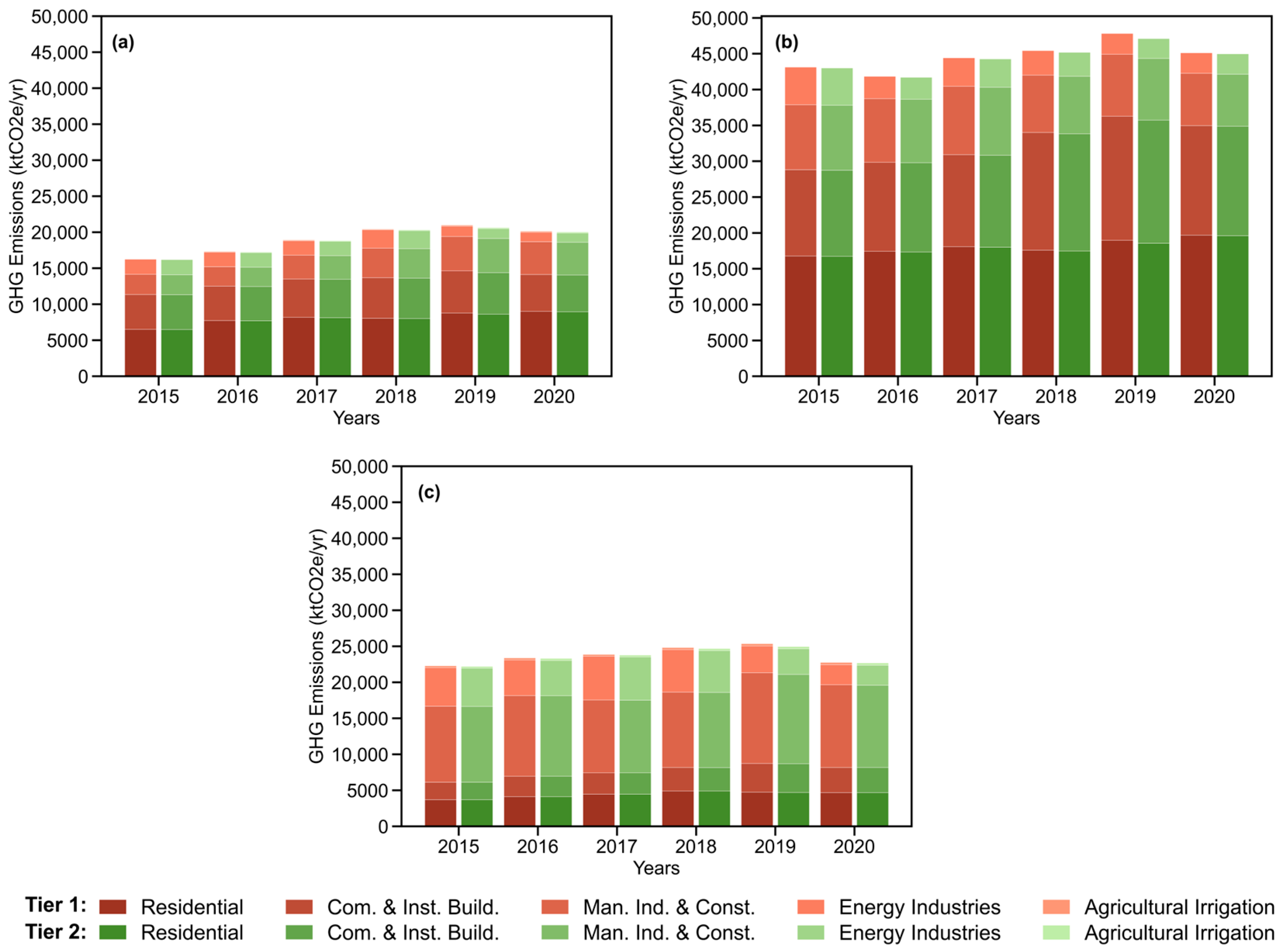
4.1. Amount of Greenhouse Gas Emissions from Stationary Combustion

In the stationary combustion sector, emissions are computed based on the consumption of natural gas, coal, fuel oil, and electricity in various activities, including energy industries, commercial/institutional buildings (in Figure 3, these are labeled ‘Com. & Inst. Build.’), residential buildings, and agricultural, forestry, and fishing activities. Figure 3 illustrates the emissions results obtained through the application of Tier 1 and Tier 2 approaches in the provinces of Ankara, Istanbul, and Izmir. The emissions calculations using both approaches exhibit remarkable similarity in all three metropolitan areas. While there was an upward trend in emissions from 2015 to 2019 across all cities, a decline in emissions was observed in 2020. Among the contributing factors to this trend, it can be demonstrated that, in Istanbul and Izmir, there was a reduction in electricity and natural gas consumption in the industry, energy sector, and commercial/government buildings compared to 2019. Additionally, there was a decrease in coal consumption in residences in 2020. In Ankara, the decline in fuel oil consumption in residences, as well as reduced natural gas and electricity consumption in commercial buildings, and a decrease in natural gas consumption in the industry and energy sector, can be identified as contributing factors. Across all three metropolitan areas, the highest emissions occurred in 2019.

In terms of an overall annual comparison, it becomes evident that Istanbul contributes to 51% of the total emissions from stationary combustion, followed by Izmir with 27%, and then Ankara with 22%. Specifically, in Istanbul, the residential sector emerges as the leading contributor to GHG emissions, accounting for an average of 41% across all years (Table S9). This outcome is notably influenced by excessive natural gas and electricity consumption in residential buildings. In 2020, emissions attributed to natural gas and electricity consumption in residential buildings in Istanbul [137] amounted to 10,210.3 ktCO₂e and 9063.8 ktCO₂e, respectively. The number of residential subscribers in Istanbul has been consistently increasing each year, and the correlation between this and natural gas consumption has been calculated at 0.92. Furthermore, meteorological conditions exert an influence on natural gas consumption, consequently impacting emissions. A correlation can be observed between the reduction in heating degree days (HDDs) in Istanbul in 2018 (Table S10) and the corresponding decrease in natural gas consumption [110,138]. Similarly, a linear relationship can be established between consumption in industrial and commercial buildings and HDDs. However, the decline in consumption in both sectors in 2020 is presumed to be more attributable to the COVID-19 pandemic than to HDDs. It is noteworthy that the commercial sector holds significant economic importance for Istanbul, contributing to 27% of the country’s total. As illustrated in Figure 3, emissions from commercial and official buildings exhibit the highest average percentage in Istanbul, amounting to 63% overall years. Despite possessing productive agricultural lands, Istanbul trails behind in agricultural production [111]. The city’s emphasis on the service and industrial sectors has resulted in limited agricultural activities, leading to significantly lower emissions from agricultural irrigation compared to other cities. Additionally, the assumed less significant impact on emissions from the industrial sector, due to the unavailability of data on coal or other fossil FC, contributes to this trend.

When compared to other cities, it is evident that Izmir exhibits the highest emissions in the industry and energy sector, with a rate of 47% (Table S11). Notably, Izmir stands out as the sole city among the three metropolitan areas that generates sufficient electricity to meet its own demands. Furthermore, Izmir possesses substantial potential for renewable energy sources, resulting in a notable share of renewable energy in electricity production. Izmir, responsible for 7% of the country’s industrial production, also harbors Türkiye’s most significant export port [139]. The highest emissions from the industrial sector were recorded as 12,600.6 ktCO₂e in 2019, primarily attributed to the consumption of natural gas and electricity. In the energy industry, the peak emissions occurred in 2017 due to natural gas consumption. Notably, in both sectors, fossil FC decreased, leading to a subsequent decline in GHG emissions in 2020. Izmir’s Mediterranean climate, characterized by a higher annual average temperature than other cities (Table S12), results in reduced reliance on fossil fuels for heating purposes in households [137]. In Izmir, an average of 4450.9 ktCO₂e yr⁻¹ (Tier 1) and 4435.8 ktCO₂e yr⁻¹ (Tier 2) emissions were generated from residential buildings between 2015 and 2020. This represents an average of 22% of emissions from residential buildings compared to other cities (Table S11). Moreover, Izmir possesses significant agricultural potential, and its fertile agricultural lands contribute to higher emissions from agricultural irrigation compared to other cities [139].

Compared to other cities, the total emissions from stationary combustion in Ankara were lower between 2015 and 2020 (Table S13). Similar to Istanbul, the highest emissions in Ankara also originate from residential buildings, constituting 42% of total emissions. As observed in other cities, there was a correlation between the observed decrease in HDDs (Table S14) and the reduction in natural gas consumption in 2018 [110,137]. Emissions from the industrial, energy, and commercial sectors showed a consistent increase between 2015 and 2019 but experienced a decline in 2020, likely attributable to the impact of the COVID-19 pandemic. In a survey of firms predominantly from Istanbul, Ankara, and Izmir, 41% of the participating firms reported significant impacts from COVID-19 by the end of 2020, while 35% experienced somewhat lesser effects. The survey also indicated that micro and small-scale firms were more susceptible to the adverse effects of the pandemic [140]. In Ankara, approximately three-quarters of the population are employed in the service sector, encompassing civil service, commerce, transportation, and communication, while one-quarter is engaged in the industrial sector, and 2% work in agriculture. Due to the substantial presence of the service sector, emissions from commercial and official institutions have surpassed other sources following residential areas. Within this sector, an annual average of 5258.9 ktCO₂e (Tier 1) and 5236.1 ktCO₂e (Tier 2) emissions were recorded between 2015 and 2020. Emissions attributable to agricultural irrigation constitute only 1% of the total emissions. The predominance of the service and industrial sectors in the city, coupled with the limited agricultural activity, may have contributed to this outcome.

Figure 3. GHG emissions (ktCO₂e yr⁻¹) from stationary combustion for (a) Ankara, (b) Istanbul, and (c) Izmir.

Figure 3. GHG emissions (ktCO₂e yr⁻¹) from stationary combustion for (a) Ankara, (b) Istanbul, and (c) Izmir.

4.2. Amount of Greenhouse Gas Emissions from Mobile Combustion

Emissions from mobile combustion have been determined based on the quantity of FC in road, air, sea, and rail activities (Figure 4). The fuels encompassed within this category include gasoline, diesel, LPG, aviation gasoline, and jet fuel [137]. When comparing the three cities, it is evident that the highest emissions occur in Istanbul. Due to insufficient data, the Tier 2 method was only applied to road and air transport. Analyzing Istanbul’s Tier 1 results reveals a decrease in FC in all transportation vehicles in 2020, leading to a 14% reduction in emissions compared to 2019 (Table S15). Notably, the road transportation sector consistently contributes the highest emissions across all years. The emission impact arising from both intra-city and transit traffic in road transportation was quantified, constituting approximately 90% of the total emissions. Particularly in the years 2018–2020, there was a notable reduction in emissions attributable to road transportation, with a significant decrease observed in 2020. Istanbul’s intra-city transportation benefits from a more extensive rail system network compared to other cities. However, due to a lack of data on electricity consumption by the High-Speed Train (HST) and Marmaray traversing Istanbul, emissions calculations were exclusively based on diesel FC [141]. Moreover, annual electricity consumption data for the metro, cable car, tram, and funicular were acquired, and emissions calculations were conducted accordingly. Consequently, emissions stemming from electricity consumption in the railway sector account for 91% of the total railway emissions. Although emissions from rail transportation peaked in 2019, a decline occurred in 2020 due to reduced usage of metro, cable car, and train services during the pandemic. The lower FC in the water-borne navigation sector led to lower emissions compared to other sectors. The highest emissions from the aviation sector are also observed in Istanbul. While emissions in Istanbul remained quite similar in the years 2015–2019, a notable 40% decrease was observed in 2020. According to the Tier 2 approach, Istanbul ranks first in terms of the number of vehicles on the road in Türkiye. Additionally, although the emissions from road transportation increased between 2015 and 2017, a subsequent decline has been observed since 2018. It was observed that Tier 1 results for road transportation are 17% higher than Tier 2. The Tier 1 calculation involves more generalization compared to Tier 2, as it overlooks the individual technical specifications of each vehicle and the variation in emissions associated with different combustion technologies. Consequently, the higher results in Tier 1 are considered reasonable. Istanbul boasts three active airports [111]. The highest fuel consumption and, consequently, GHG emissions during LTO activities occurred in 2016. The travel restrictions imposed due to the pandemic in 2020 had a mitigating effect on aviation FC and the related emission levels.

Ankara ranks as the city with the second-highest mobile source emissions following Istanbul. According to Tier 1 calculations, there was an upward trend in emissions from 2015 to 2018, peaking at 9166.4 ktCO₂e in 2018. Throughout all years, road transport accounted for the highest emissions, averaging 91%. Despite having an airport, air transport emissions are nearly half of Istanbul’s emissions, influenced by aviation FC. The maximum emissions occurred in 2016 at 1021.4 ktCO₂e. Similar to road transport, air transport emissions experienced a 43% decrease in 2020 compared to the previous year, attributed to travel restrictions imposed by the pandemic.

Owing to its distance from the coast, railways have historically played a crucial role in transportation in Ankara [142]. Due to the absence of data on electricity consumption for the High-Speed Train (HST) and Başkentray, only diesel FC has been considered. Moreover, emissions from the city’s metro and cable car lines were computed based on electricity consumption. Over the period 2015–2020, railway emissions have exhibited relative stability, with emissions remaining consistently close to each other. Emissions from railways reached their zenith in 2019 but experienced a decline in 2020, mirroring trends observed in other cities, attributable to reduced usage of metro, cable car, and train services. Total emission levels under Tier 2 are consistently around 20% lower than those calculated under Tier 1. Specifically focusing on road transport, Tier 1 estimates are 24–31% higher across all years. In Ankara, the aircraft types with the highest number of takeoffs and landings throughout all years include A320, A321, B737, and B738. The year exhibiting the highest Tier 2 emissions from aviation was 2016 (Table S16).

Emission levels from mobile combustion in Izmir are comparatively lower than in other cities. As observed in similar urban contexts, the peak emission occurred in 2018, with a Tier 1 calculation yielding 6208.5 ktCO₂e. The preponderance of emissions in Izmir emanates from road transportation, constituting approximately 92% of the total, followed by air transportation. Notably, air transportation emissions, which experienced an upward trend from 2015 to 2018, witnessed a significant decline in 2020. Emissions resulting from passenger and freight transportation via IZBAN (diesel), metro, and tramway lines (electric) were computed based on FC and were determined to be notably lower than those arising from road transportation. In contrast to trends observed in other transportation sectors, emissions from maritime transportation experienced an increase in 2020 (Table S17). Tier 2 results revealed a 20% reduction in emissions from road transportation compared to Tier 1, while emissions from air transportation remained relatively stable.

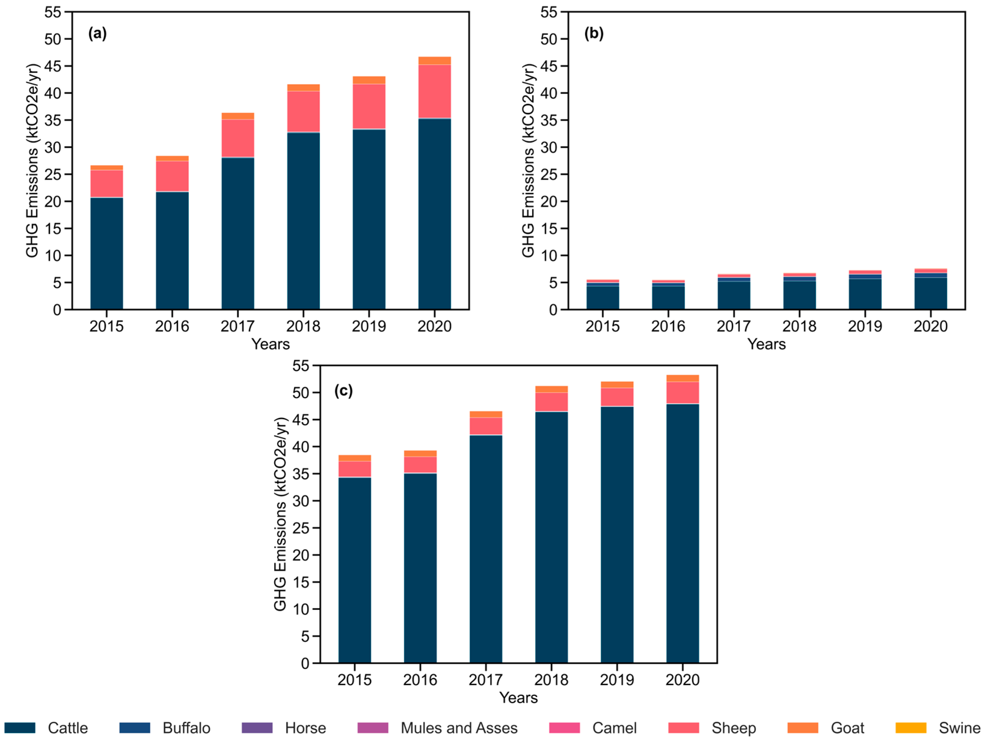
4.3. Amount of Greenhouse Gas Emissions from Enteric Fermentation

CH₄ emissions stemming from enteric fermentation in animals were assessed using the Tier 1 method, considering the animal species (Table S18). This approach was chosen due to the unavailability of gross energy intake data for animals in different categories specific to each country. As illustrated in Figure 5, emissions from this sector are most pronounced in Izmir and least in Istanbul. There has been a consistent increase in emissions across all cities from year to year. In Izmir, emissions from animal production constitute 46.6%, crop production accounts for 42.36%, and aquaculture contributes 11.04% to the overall emissions. Izmir boasts more productive land, a larger population of animals, and a more diverse array of crops compared to other cities. The dairy and dairy products sector stands out as the most significant contributor to the Izmir economy. In 2019, the city was home to 780 thousand cattle, 671 thousand sheep, and 242 thousand goats [139]. Emissions from cattle constitute 90% of the total emissions, followed by domestic sheep at 7%. Cattle in Izmir take the lead among all animals, commanding a 43% share, followed by domestic sheep with 41% and goats with 16% [64]. The elevated emissions from cattle can be attributed to their comprising 43% of the total animal population, and their enteric fermentation emissions surpass those of other animals. A comparable scenario is observed in Ankara, where cattle emissions contribute to 77% of the total, with sheep emissions constituting 19%. Despite a higher number of sheep in the city, cattle emissions take precedence due to the higher EF of the cattle species. In Istanbul, domestic sheep take the lead with a rate of 46%, while cattle follow closely with a rate of 37%. However, akin to other cities, the predominant emissions (78%) originate from cattle species, with buffalo species contributing 11% (Figure 5).

4.4. Amount of Carbon Accumulation in the Forest Land

Carbon sequestration in forests is predominantly observed in biomass, dead litter/wood, and soil. The foundational data for this study were obtained from comprehensive forest management plans encompassing the periods of 2010–2020 for Ankara, 2010–2020 for Izmir, and 2011–2021 for Istanbul. Through personal interviews with provincial forest directorates, the management plans for Ankara reveal a broadleaved productive forest stock of 1,044,248.2 m³, a coniferous productive forest stock of 23,498,967.9 m³, a broadleaved degraded forest stock of 511,000 m³, and a coniferous degraded forest stock of 475,000 m³. In Ankara, the dominant tree species is black pine, constituting 44%, followed by oak at 36%, and scotch pine at 10%. The volume increment in Ankara’s forests is 634,637 m³ for productive forests and 25,892 m³ for degraded forests. In Istanbul, the management plan indicates an 8,184,595 m³ stock for broadleaved productive forests, 5,741,289 m³ for coniferous productive forests, and 123,000 m³ for broadleaved degraded forests. The volume increment for productive forests in Istanbul is 643,620 m³, with a corresponding value of 2421 m³ for degraded forests. Throughout the province, oak trees dominate with a rate of 47%, followed by mixed-leaved trees at 33%, and maritime pine trees at 6%. While 44% of Istanbul’s area is covered by forests, the remaining 56% constitutes non-forested land [125]. In Izmir, the broadleaved productive forest stock is 919,000 m³, the coniferous productive forest stock is 47,407,220 m³, the broadleaved degraded forest stock is 1,290,186 m³, and the coniferous degraded forest stock is 839,714 m³. While 40% of Izmir is covered by forests, the remaining 60% constitutes non-forest land. İzmir’s forests are dominated by 46% Turkish pine, 37% other species, and 11% oak. The volume increment value in İzmir’s forests is 850,922 m³ for productive forests and 58,816 m³ for degraded forests. The results regarding the amount of carbon stored in urban forests are provided in

Table 8. Total biomass and carbon storage in metropolitan forests (t).

Carbon Pool	Tree Type	Ankara (2010)		Istanbul (2011)		Izmir (2010)
		Productive Forest	Degraded Forest	Productive Forest	Degraded Forest	Productive Forest	Degraded Forest
AGB	Coniferous	12,702,414.1	256,806.6	3,103,465.3	0	25,626,067.6	453,909.1
	Broadleaved	740,069.2	362,480.3	5,800,504.3	87,357.7	651,523.5	914,367.7
BGB	Coniferous	3,683,700.1	102,722.6	900,004.9	0	7,431,559.6	181,563.6
	Broadleaved	177,616.6	166,740.9	1,392,121.0	40,184.6	156,365.6	420,609.2
∆CAGB	Coniferous	6,478,231.2	130,971.4	1,582,767.3	0	13,069,294.5	231,493.6
	Broadleaved	355,233.2	173,990.5	2,784,242.1	41,931.7	312,731.3	438,896.5
∆CBGB	Coniferous	1,878,687.0	52,388.5	459,002.5	0	3,790,095.4	92,597.5
	Broadleaved	85,256.0	80,035.6	668,218.1	19,288.6	75,055.5	201,892.4
DWC	Coniferous	59,701.3	1207.0	14,586.3	0	120,442.5	2133.4
	Broadleaved	3478.3	1703.7	27,262.4	410.6	3062.2	4297.5
DLC	Coniferous	1,275,153.1	137,228.2	362,310.2	0	1,298,563.9	121,996.3
	Broadleaved	135,907.3	108,275.6	661,484.8	14,215.1	116,279.1	189,580.1
Organic carbon in soil	Coniferous	13,086,558.1	1,412,122.4	3,718,293.3	0	13,326,817.0	1,255,381.8
	Broadleaved	3,074,041.8	2,468,218.5	14,961,904.6	324,042	2,630,078.9	5,576,992.6
Total Carbon		30,998,388.8		25,639,959.4		41,602,300.1

, indicating that the highest carbon accumulation occurs in Izmir, followed by Ankara and Istanbul.

Carbon storage values between 2010–2020 were calculated using increment values (

Table 9. Total and annual carbon storage in metropolitan forests (t).

Years	Ankara		Istanbul		Izmir
	Total Carbon	Annual Stored Carbon	Total Carbon	Annual Stored Carbon	Total Carbon	Annual Stored Carbon
2020	37,409,350.9	260,065.9	27,958,836.1	253,345.4	49,217,307.3	905,359.3
2019	37,149,285.0	260,065.9	27,705,490.7	330,895.0	48,311,948.1	905,359.3
2018	36,889,219.1	338,271.6	27,374,595.7	330,895.0	47,406,588.8	635,747.2
2017	36,629,153.3	338,271.6	27,043,700.7	330,895.0	46,770,841.6	635,747.2
2016	36,369,087.4	338,271.6	26,712,805.8	188,827.7	46,135,094.4	635,747.2
2015	35,874,404.3	1,451,961.2	26,523,978.1	188,827.7	45,499,347.2	1,059,413.8
2014	35,614,338.4	1,451,961.2	26,335,150.3	188,827.7	44,439,933.4	1,059,413.8
2013	35,354,272.6	1,451,961.2	26,146,543.9	253,292.3	43,380,519.7	1,059,413.8
2012	31,518,520.6	260,065.9	25,893,251.6	253,292.3	42,321,105.9	359,402.9
2011	31,258,454.7	260,065.9	25,639,959.4		41,961,703.0	359,402.9
2010	30,998,388.8				41,602,300.1

). However, due to the unavailability of diameter values and increment values for each tree species, it is assumed that all tree diameters remained within the same diameter range, and thus, they experienced the same rate of growth over eleven years. These values do not precisely reflect the actual values since there is an increment in the total diameter. They are calculated solely to demonstrate the average amount of carbon that can be stored in one year. It is estimated that there will not be significant changes in forest areas in Istanbul over the years, and only minor differences in annual carbon storage values will be observed. In Ankara and Izmir, however, the area of productive forests has increased, and the area of degraded forests has decreased over the years. Particularly between 2012–2015, the area of productive forests had increased by 17%. Due to these changes, it is estimated that more carbon storage was achieved between 2012–2015.

4.5. Amount of Greenhouse Gas Emissions from Waste Sector

The emissions from the waste sector in Ankara, Istanbul, and Izmir were calculated based on CH₄ emissions from SWD sites and emissions from composting in Istanbul. The amount of emissions from SWD has shown minimal change over the years in Figure 6.

Istanbul exhibits the highest emissions among the three cities in Table S19. It is noteworthy that there is no unsanitary disposal in Istanbul. The CH₄ gas released from landfill gas in the sanitary landfill sites undergoes collection and is converted into electricity at the Electricity Energy Generation Facility from Landfill Gas. Istanbul Metropolitan Municipality (IMM) accrues carbon credits by generating electricity from landfill gas. Based on personal interviews with IMM, it was determined that the gas collection efficiency in the facilities in Istanbul is 75%, and the calculations are based on this rate. The results of the calculations reveal that the highest CH₄ emissions occurred in 2017, reaching 3466.3 ktCO₂e yr⁻¹. In Ankara, both unsanitary and sanitary landfill sites are in operation for solid waste disposal. Over the years, several solid waste transfer stations have been established to eliminate unsanitary disposal practices and facilitate the transportation of waste to modern recycling facilities located in the Mamak and Sincan districts [143]. Based on information obtained from the municipality, the gas collection efficiency in the facilities is reported to be 88%, and all calculations are grounded on this rate. Subsequent bilateral meetings with the municipality indicated that the annual quantity of generated waste has not undergone significant changes. The calculations suggest that the highest emissions were estimated to occur in 2016, reaching 533 ktCO₂e yr⁻¹. In Izmir, the waste management infrastructure includes the Harmandali Solid Waste Landfill Site, Bergama SWD, and the Medical Waste Sterilization Facility. The sanitary landfill sites account for over 90% of solid waste disposal, with the remaining portion being disposed of in uncontrolled dumping sites. In 2019, the Harmandali Solid Waste Landfill Site in Izmir initiated electricity production from landfill gas [143]. The gas collection efficiency in the facilities is reported to be 90%, forming the basis for all calculations. The estimations indicate that the highest emissions were observed in 2020, reaching 470 ktCO₂e yr⁻¹. Similar to Ankara, there was minimal fluctuation observed in the volume of emissions from SWD over the years.

It has been determined that compost production was not conducted in Ankara during the years of the study. Similarly, In Izmir, a compost unit was established at the Harmandali Facility starting in 2020. Consequently, the emission related to composting was not included in the study for Izmir. In Istanbul, compost has been generated from organic waste sourced from markets, kitchens, parks, and gardens at the Kemerburgaz Recycling and Composting Plant and Şile-Kömürcüoda Integrated Mechanical Biological Treatment and Recycling Facilities since 2001 [143]. Assessing emissions from composting requires consideration of both the incoming waste volume and the recovered waste amount. In 2017, lower CH₄ and N₂O emissions were recorded due to a reduction in the waste entering the facility compared to other years and an increase in the amount of waste recovered. When analyzed in terms of CO₂e, CH₄ emissions account for 64%, while N₂O emissions constitute 36% across all years (

Table 10. Emissions from composting in Istanbul (ktCO₂e yr⁻¹).

Years	CH4	N2O	Total
2020	12.16	6.90	19.06
2019	11.50	6.53	18.03
2018	13.53	7.69	21.22
2017	8.99	5.10	14.09
2016	14.25	8.09	22.34
2015	14.35	8.15	22.5

).

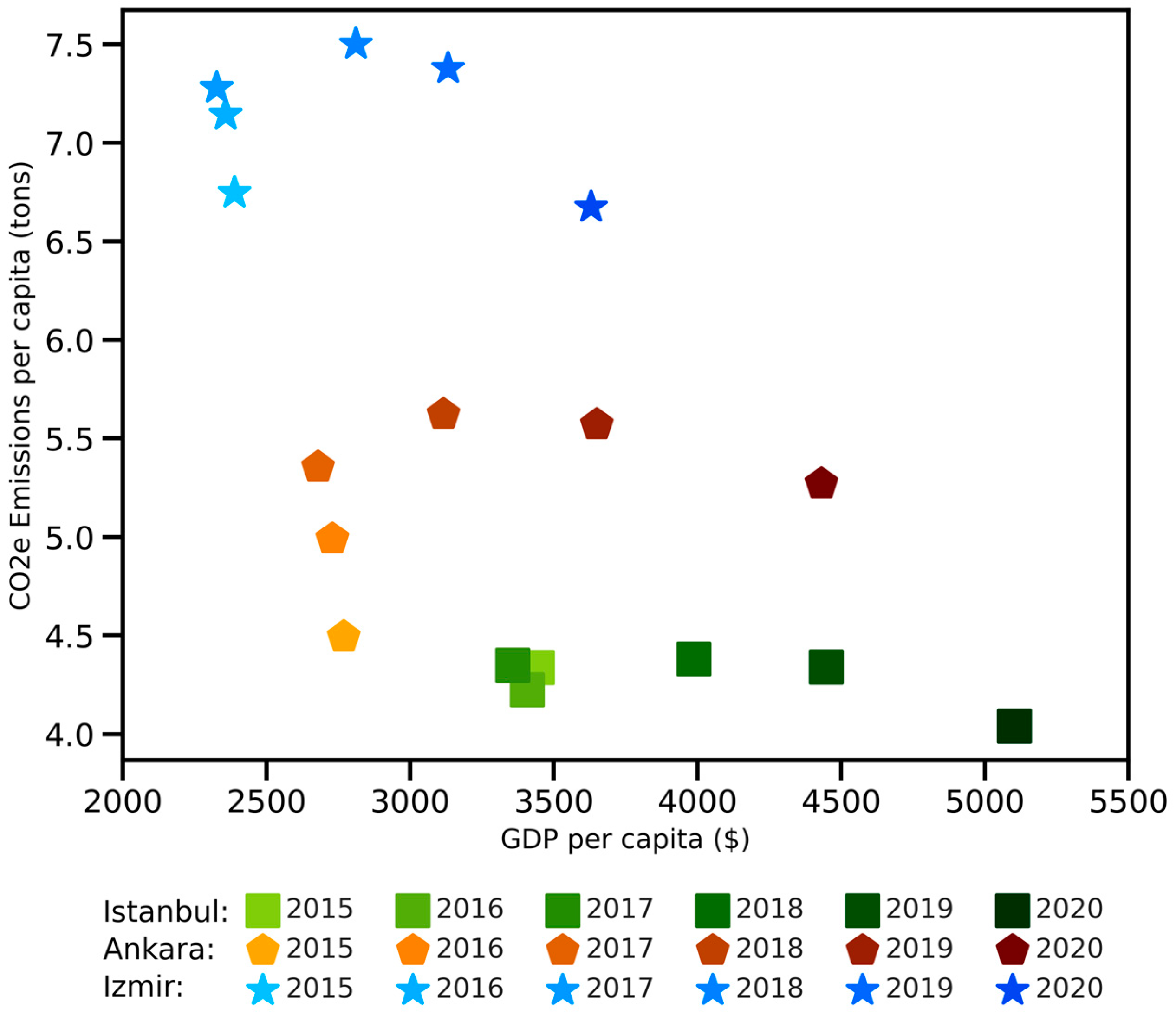
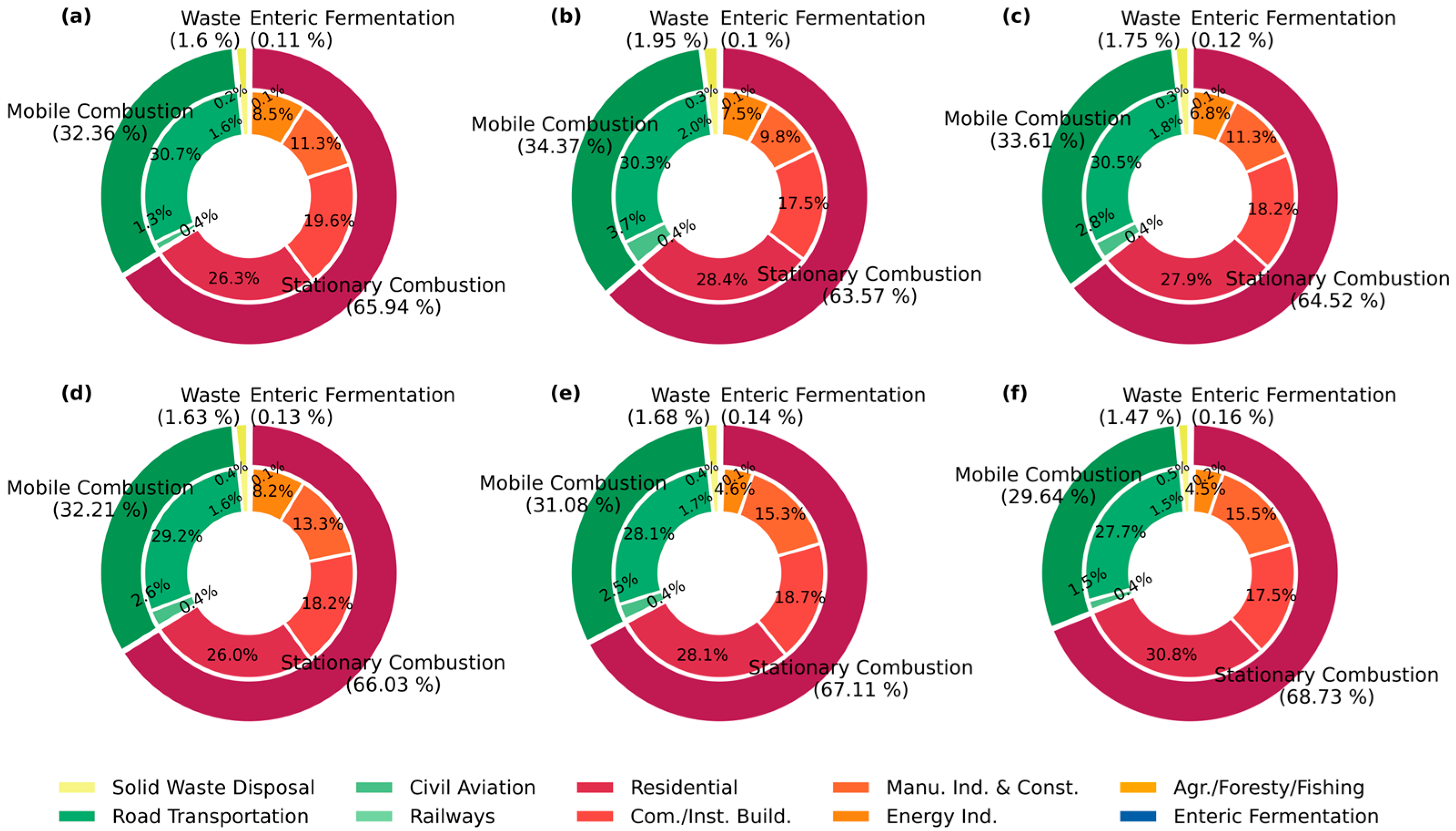
4.6. City-Based Comparisons

According to the Tier 1 approach calculations, it is evident that the predominant source of total emissions is Istanbul, while the annual total emissions from Ankara and Izmir exhibit similarities (Table S20). GHG emissions are influenced by factors such as population and economic activities. A comparative analysis of emission calculations was conducted for the three largest cities in Türkiye based on population and GDP, and the results are depicted in Figure 7. Per capita emission levels in Istanbul, leading in terms of GDP in Türkiye, are consistently lower than those in the other cities for each year. Conversely, in Izmir, characterized by a lower population and GDP, per capita GHG emissions are higher compared to the other cities (Table S21).

The contribution of different sectors to total emissions exhibits variation across all cities as given in Figure 8, Figure 9 and Figure 10. Figure 8, generated using Tier 1 results, illustrates that stationary combustion consistently emerges as the dominant sector when analyzing Ankara for all years. For instance, the sector, which had a 65.94% impact in 2015, increased to 68.73% in 2020. Following this sector, mobile combustion, waste, and enteric fermentation contribute to the emissions profile. In Ankara, the energy sector is a primary source of emissions compared to other sectors, while emissions attributed to waste and enteric fermentation remain comparatively lower. Similar to Ankara, in Istanbul, it is apparent that emissions from stationary combustion constitute the predominant sector, as illustrated in Figure 9. In comparison to Ankara, the proportion of emissions from stationary sources and waste is higher in Istanbul, while mobile sources and enteric fermentation contribute to a lesser extent. The impact of mobile sources, which accounted for a 28.98% share in 2015, decreased to 24.06% in 2020. Conversely, stationary sources increased from 66.32% in 2015 to 71.21% in 2020.

In Figure 10, an analysis of the influence of various sectors on overall emissions in Izmir reveals that stationary sources, particularly the industrial sector, contribute significantly more than other sectors and even exceed the contributions observed in other cities. For instance, the impact of the industrial sector on emissions, with a share of 37% in 2015, escalated to 39.5% in 2020. Consistent with trends in other cities, the impact of mobile sources, waste, and enteric fermentation follows stationary sources in order.

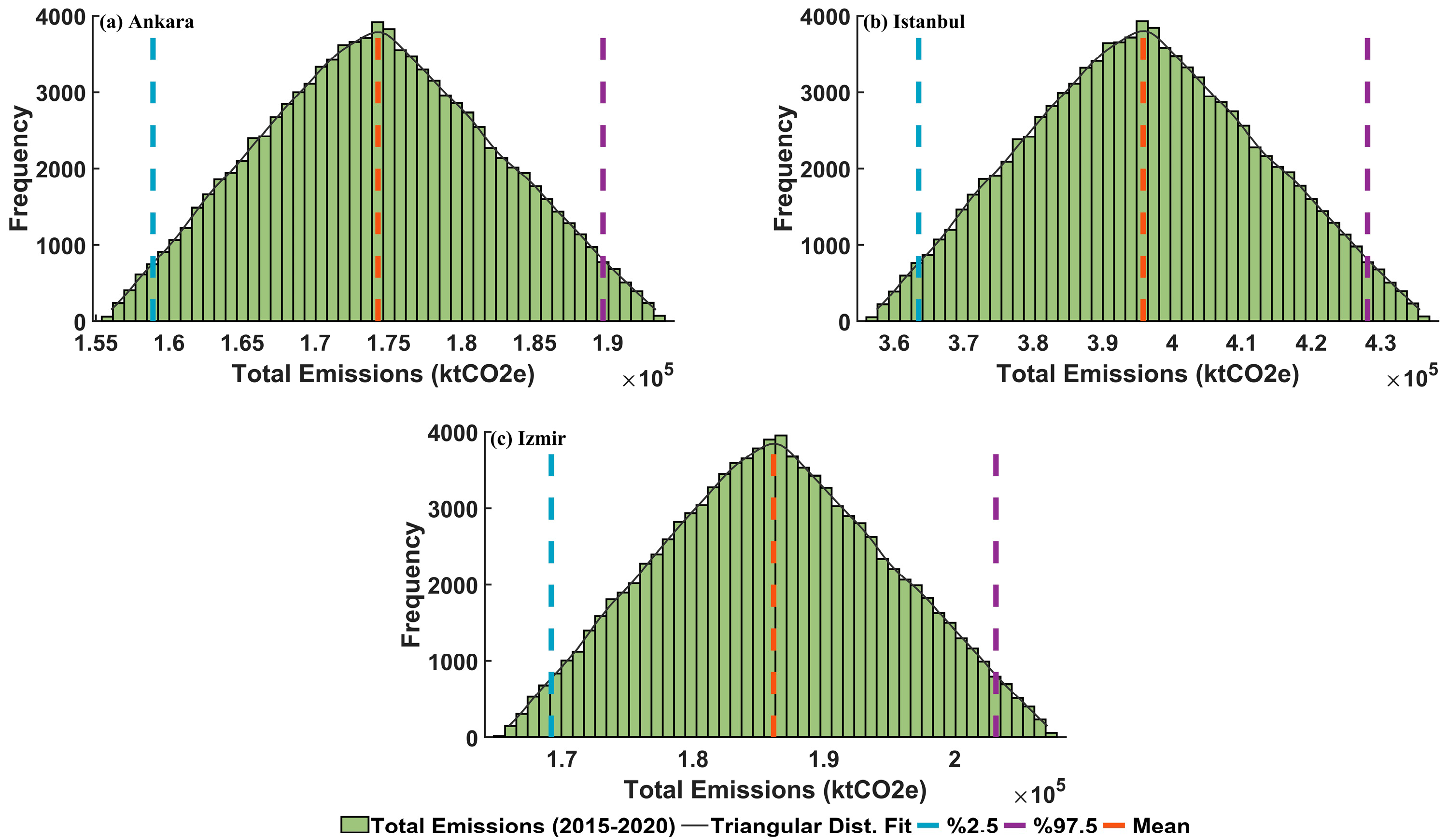
4.7. Monte Carlo Simulation

In the process of creating GHG inventories, uncertainties arise from assumptions made, double counting, some conceptual errors, or uncertainties resulting from a lack of information. Reducing these uncertainties is crucial for inventory results because the accuracy and reliability of inventory results are essential for future studies and climate change mitigation efforts. The main reason for uncertainties in the inventory process is variability in activity data and EFs. Activity data for different sectors such as stationary and mobile combustion, SWD in landfills, composting, and enteric fermentation have different uncertainty rates. Uncertainty rates for activity data were assumed to be ±10% for the stationary combustion sub-sector, ±5% for the mobile combustion sub-sector, and ±20% for the enteric fermentation sub-sector [113]. Additionally, different fuel consumptions (coal, natural gas, fuel oil, diesel, gasoline, etc.) exist for stationary and mobile combustion sectors. Emissions of CO₂, CH₄, and N₂O to the atmosphere due to these consumptions were calculated using an average EF value provided by the IPCC. Only country-specific CO₂ EFs were obtained for some natural gas and coal. Additionally, when calculating emissions from composting, IPCC’s CH₄ and N₂O EFs were used (Table S8). For this reason, it is felt that the results of these calculations will yield a result close to the actual emission quantities rather than being exact. As long as there are no specific EFs for the country or even the city, providing emission ranges will be more reliable as it would yield results close to actual emissions. Hence, in this study, MCS has been employed for this purpose.

The MCS was exclusively conducted for emissions derived from the Tier 1 method due to the unavailability of data for Tier 2 in most sectors. To enhance sensitivity, a simulation comprising 100,000 iterations was executed to address emission uncertainties. Triangular distribution was employed for uncertainties, with data defined within the 95% confidence interval recommended by the IPCC. The comprehensive results, encompassing the total mean, maximum, and minimum emission amounts that Ankara, Istanbul, and Izmir could potentially release into the atmosphere during the years 2015–2020, within a 95% confidence interval, are visually represented in Figure 11. Based on calculations that consider uncertainties and error margins, the total atmospheric emissions for the years 2015–2020 were estimated to average 174,289.3 ktCO₂e in Ankara, 395,816.8 ktCO₂e in Istanbul, and 186,168.3 ktCO₂e in Izmir. Within a 95% confidence interval, it is projected that in Ankara, the minimum emissions for the years 2015–2020 will be 158,905.7 ktCO₂e, and the maximum emissions will be 189,673 ktCO₂e. In Istanbul, the minimum emissions are estimated to be 363,532.8 ktCO₂e, and the maximum emissions are estimated to be 428,100.7 ktCO₂e. In Izmir, the minimum emissions are projected to be 169,188.1 ktCO₂e, while the maximum emissions are expected to be 203,148.4 ktCO₂e.

The results of the MCS presented in Table S22 indicate that Istanbul consistently has the highest emissions for all years, followed by Izmir until the year 2020. Surprisingly, in the year 2020, the average emission amount in Ankara surpassed that of Izmir. While there is an overall increasing trend in the emission amount from year to year in Ankara and Izmir, there was a notable decrease in Izmir in 2019 and 2020, and in Ankara in 2020. Conversely, in Istanbul, lower emissions were observed in both 2016 and 2020 compared to the previous year. When considering all the years, the highest emissions in Ankara were observed in 2019. According to the 95% confidence interval, it is projected that in 2019, emissions in Ankara will vary between a minimum of 29,037.8 ktCO₂e and a maximum of 34,587 ktCO₂e. Similarly, Istanbul exhibited the highest emissions in 2019, with an estimated range from a minimum of 63,570.9 ktCO₂e to a maximum of 74,825.3 ktCO₂e. The peak emissions in Izmir were recorded in 2018, and within a 95% confidence interval, it is predicted that emissions in Izmir during that year will fall within a range from a minimum of 29,780.6 ktCO₂e to a maximum of 35,716.6 ktCO₂e. A comparative analysis with the findings presented in Table S20 reveals that the total emission quantities derived from the study consistently fall below the average results obtained from the MCS across all cities for all years. Throughout the study, it is thought that employing EFs specific to Türkiye, in lieu of default EFs utilized in the Tier 1 method, and addressing all uncertainties in activity data through robust calculations based on reliable data, would contribute to the establishment of a more accurate emission inventory for cities in Türkiye. However, even in this current study, MCS demonstrates that the obtained results consistently fall within the 95% confidence interval.

5. Conclusions

This study calculated GHG emissions from various sectors and carbon sequestration in trees for Ankara, Istanbul, and Izmir from 2015 to 2020. Upon scrutiny of the cumulative emission levels during the mentioned period, Istanbul had the highest emissions (387.3 thousand ktCO₂e), followed by Ankara (171.7 thousand ktCO₂e) and Izmir (183.4 ktCO₂e). A noteworthy observation across all regions experienced decreased emissions in year 2020 due to the COVID-19 pandemic. When analyzing all calculations by sector:

Stationary combustion emissions, assessed using Tier 1, surpass Tier 2 outcomes across all years and cities, with Istanbul demonstrating the highest emissions. Notably, in Istanbul, 26% of emissions are linked to electricity consumption in commercial and institutional buildings, while the lowest emissions stem from electricity used for agricultural irrigation. This emission pattern aligns with the city’s commercial prominence and numerous official institutions. Despite having fertile agricultural lands, the prevalence of service and industrial sectors has curtailed agricultural activities, leading to lower emissions from agricultural production compared to other sectors. In comparison to Ankara, Izmir demonstrated higher emissions from stationary combustion. The primary reason for this discrepancy is the higher consumption of natural gas and electricity in the industrial sector of Izmir. Additionally, Izmir exhibits the highest emission levels attributed to agricultural irrigation. Despite its agricultural productivity, Izmir experiences insufficient or irregular rainfall during the summer months, necessitating increased irrigation and consequently raising the consumption of water and energy. Emissions originating from residential areas, directly correlated with population density, are most pronounced in Istanbul, followed by Ankara. In Izmir, characterized by comparatively warmer climate conditions, emissions related to heating during winter are notably lower than in other cities. The trend indicates an increase in emissions from this sector between 2015 and 2019, with a subsequent decrease in 2020, primarily attributed to the impact of the pandemic.

In Tier 1 calculations, Istanbul exhibits the highest mobile combustion emissions, with Ankara following closely. Road transportation emerges as the predominant source of emissions in all cities, followed by air, railway, and maritime transportation. The three cities, particularly Istanbul, have advanced railway networks, encompassing diesel consumption in intercity railways and electric usage in intracity vehicles. Tier 2 results corroborate the dominance of road transportation emissions. The growing number of road vehicles in all three cities has led to an escalation in emissions within this sector. Assessing aviation emissions reveals the B738 aircraft type, with the highest number of takeoffs and landings, has lower fuel consumption and GHG emissions during operations. While relatively eco-friendly, the B738’s disproportionately high number of LTO contributes to about 50% of total emissions. Similar to stationary combustion trends, mobile combustion emissions also declined in 2020 due to pandemic-related travel restrictions and lockdowns.

Emissions from the waste sector, specifically derived from SWD and composting, have undergone calculation. The absence of composting practices in Ankara and Izmir from 2015 to 2020 has been established. Discrepancies in emissions related to the disposal of solid waste in sanitary landfills are attributable to variances in population, solid waste composition, and gas collection efficiencies within disposal facilities among the cities. Notably, Istanbul has been identified as the city with the highest emission levels. CH₄ emissions in Ankara and Izmir exhibited similarity. Moreover, emissions from composting activities in Istanbul are 99% lower than those emanating from SWD.

Emissions from enteric fermentation were found to be higher in Izmir, owing to its more productive soil, larger livestock population, and greater variety of products compared to other cities. Conversely, Istanbul exhibited the lowest emissions in this regard. Across all cities, there was a year-by-year increase in emissions, with cattle identified as the primary contributor to the highest emission levels.

The carbon storage of trees was assessed using data from the 2010–2020 management plans. The estimations indicate that up to 2010, the forests in Ankara sequestered a total of 31 million tons, while in Izmir, the figure was 41.6 million tons, and in Istanbul, it reached 25.6 million tons. Notably, in Izmir, the presence of more productive forest areas and a higher increment value compared to other cities is anticipated to result in greater carbon sequestration capabilities, surpassing those of other provinces.

The variability in activity data and EFs introduces uncertainties into the emission inventory process. Due to the absence of EFs specific to countries or even cities, presenting emission quantities as a range would be more accurate. To enhance the sensitivity of this study, a MCS with 100,000 iterations was conducted to address uncertainties in emissions. The study provides the total emissions that Ankara, Istanbul, and Izmir could release into the atmosphere within a 95% confidence interval for the years 2015–2020. The results suggest that emissions calculated using the Tier 1 method are lower than the average emissions obtained from the MCS results.

The study on Türkiye’s three major cities is expected to aid local administrations and policymakers in their climate change mitigation efforts. Given Türkiye’s commitment to agreements like the Paris Agreement and its emission reduction obligations, conducting accurate emission calculations becomes crucial. The authentic data-based calculations will enhance awareness of GHG emission challenges in these urban centers, providing strategic guidance to policymakers. The sector-specific results of this study can help prioritize sectors for emission reduction initiatives, contributing to a more realistic approach in the global fight against climate change.

References

1. Rahman, M.I. Climate change: A theoretical review. Interdiscip. Descr. Complex Syst. 2023, 11, 1–13. [Google Scholar] [CrossRef]
2. Fanelli, C. Climate Change: ‘The Greatest Challenge of Our Time’. Altern. Routes A J. Crit. Soc. Res. 2014, 25, 15–31. [Google Scholar]
3. Hasbach, P.H. Therapy in the face of climate change. Ecopsychology 2015, 7, 205–210. [Google Scholar] [CrossRef]
4. Cianconi, P.; Betrò, S.; Janiri, L. The impact of climate change on mental health: A Systematic Descriptive Review. Front. Psychiatry 2020, 11, 74. [Google Scholar] [CrossRef]
5. Dodman, D. Blaming cities for climate change? an analysis of urban greenhouse gas emissions inventories. Environ. Urban. 2009, 21, 185–201. [Google Scholar] [CrossRef]
6. Satterthwaite, D. The implications of population growth and urbanization for climate change. Environ. Urban. 2009, 21, 545–567. [Google Scholar] [CrossRef]
7. Madlener, R.; Sunak, Y. Impacts of urbanization on urban structures and energy demand: What can we learn for urban energy planning and urbanization management? Sustain. Cities Soc. 2011, 1, 45–53. [Google Scholar] [CrossRef]
8. Solecki, W.; Seto, K.C.; Marcotullio, P.J. It’s time for an urbanization science. Environ. Sci. Policy Sustain. Dev. 2013, 55, 12–17. [Google Scholar] [CrossRef]
9. Lamb, W.F.; Creutzig, F.; Callaghan, M.W.; Minx, J.C. Learning about urban climate solutions from case studies. Nat. Clim. Chang. 2019, 9, 279–287. [Google Scholar] [CrossRef]
10. Bhardwaj, G.; Esch, T.; Lall, S.V.; Marconcini, M.; Soppelsa, M.E.; Wahba, S. Cities, Crowding, and the Coronavirus: Predicting Contagion Risk Hotspots; World Bank: Washington, DC, USA, 2020. [Google Scholar] [CrossRef]
11. Nieuwenhuijsen, M.J. Urban and Transport Planning Pathways to Carbon Neutral, livable and healthy cities; a review of the current evidence. Environ. Int. 2020, 140, 105661. [Google Scholar] [CrossRef]
12. UN DESA. Available online: https://population.un.org/wup/default.aspx?aspxerrorpath=/wup/index.htm (accessed on 25 January 2023).
13. Wang, Q.; Su, M.; Li, R.; Ponce, P. The effects of energy prices, urbanization and economic growth on energy consumption per capita in 186 countries. J. Clean. Prod. 2019, 225, 1017–1032. [Google Scholar] [CrossRef]
14. Liang, W.; Yang, M. Urbanization, economic growth and environmental pollution: Evidence from China. Sustain. Comput. Inform. Syst. 2019, 21, 1–9. [Google Scholar] [CrossRef]
15. Chen, Z.; Avraamidou, S.; Liu, P.; Pistikopoulos, E.N. Optimal design of Integrated Urban Energy System under uncertainty and Sustainability Requirements. Comput. Aided Chem. Eng. 2020, 48, 1423–1428. [Google Scholar] [CrossRef]
16. IEA. Available online: https://iea.blob.core.windows.net/assets/89d1f68c-f4bf-4597-805f-901cfa6ce889/weo2008.pdf (accessed on 13 February 2023).
17. Sovacool, B.K.; Brown, M.A. Twelve metropolitan carbon footprints: A preliminary comparative global assessment. Energy Policy 2010, 38, 4856–4869. [Google Scholar] [CrossRef]
18. Kober, T.; Schiffer, H.W.; Densing, M.; Panos, E. Global Energy Perspectives to 2060—WEC’s World Energy scenarios 2019. Energy Strategy Rev. 2020, 31, 100523. [Google Scholar] [CrossRef]
19. UN HABITAT. Available online: https://unhabitat.org/topic/urban-energy (accessed on 30 January 2023).
20. Liu, Y.; Gao, C.; Lu, Y. The impact of urbanization on GHG emissions in China: The role of population density. J. Clean. Prod. 2017, 157, 299–309. [Google Scholar] [CrossRef]
21. Driga, A.M.; Drigas, A.S. Climate change 101: How everyday activities contribute to the ever-growing issue. Int. J. Recent Contrib. Eng. Sci. IT IJES 2019, 7, 22. [Google Scholar] [CrossRef]
22. Siddik, M.A.; Islam, M.T.; Zaman, A.K.M.M.; Hasan, M.M. Current status and correlation of fossil fuels consumption and greenhouse gas emissions. Int. J. Energy Environ. Econ. Hauppauge 2020, 28, 103–118. [Google Scholar]
23. Atmaca, A.; Atmaca, N. Carbon footprint assessment of residential buildings, a review and a case study in Turkey. J. Clean. Prod. 2022, 340, 130691. [Google Scholar] [CrossRef]
24. Wigley, T.M. The pre-industrial carbon dioxide level. Clim. Chang. 1983, 5, 315–320. [Google Scholar] [CrossRef]
25. Neftel, A.; Moor, E.; Oeschger, H.; Stauffer, B. Evidence from polar ice cores for the increase in atmospheric CO2 in the past two centuries. Nature 1985, 315, 45–47. [Google Scholar] [CrossRef]
26. NASA. Available online: https://climate.nasa.gov/vital-signs/carbon-dioxide/ (accessed on 22 February 2023).
27. IPCC. Climate Change 2022: Mitigation of Climate Change. Contribution of Working Group III to the Sixth Assessment Report of the Intergovernmental Panel on Climate Change; Cambridge University Press: Cambridge, UK; New York, NY, USA, 2022. [Google Scholar]
28. Gurney, K.R.; Romero-Lankao, P.; Seto, K.C.; Hutyra, L.R.; Duren, R.; Kennedy, C.; Grimm, N.B.; Ehleringer, J.R.; Marcotullio, P.; Hughes, S.; et al. Climate change: Track urban emissions on a human scale. Nature 2015, 525, 179–181. [Google Scholar] [CrossRef] [PubMed]
29. Jacobs, J. The Economy of Cities; Vintage Books: New York, NY, USA, 1969. [Google Scholar]
30. Özsoy, C.E. Düşük karbon ekonomisi ve Türkiye’nin karbon ayak izi. Hak İş Uluslararası Emek Ve Toplum Derg. 2015, 4, 198–215. [Google Scholar]
31. Wiedmann, T.O.; Minx, J.C. A Definition of Carbon Footprint, Ecological Economics Research Trends; Pertsova, C.C., Ed.; Nova Science Publishers: Hauppauge, NY, USA, 2008; pp. 1–11. [Google Scholar]
32. Chen, R.; Zhang, R.; Han, H. Where has carbon footprint research gone? Ecol. Indic. 2021, 120, 106882. [Google Scholar] [CrossRef]
33. Peters, G.P. Carbon footprints and embodied carbon at multiple scales. Curr. Opin. Environ. Sustain. 2010, 2, 245–250. [Google Scholar] [CrossRef]
34. Plassmann, K.; Edwards-Jones, G. Carbon Footprinting and Carbon Labelling of Food Products; Environmental Assessment and Management in the Food Industry; Woodhead Publishing: Cambridge, UK, 2010; pp. 272–296. [Google Scholar]
35. Pandey, D.; Agrawal, M. Carbon footprint estimation in the agriculture sector. Assess. Carbon Footpr. Differ. Ind. Sect. 2014, 1, 25–47. [Google Scholar] [CrossRef]
36. Akyol, M.; Uçar, E. Carbon footprint forecasting using time series data mining methods: The case of Turkey. Environ. Sci. Pollut. Res. 2021, 28, 38552–38562. [Google Scholar] [CrossRef] [PubMed]
37. Paravantis, J.A.; Tasios, P.D.; Dourmas, V.; Andreakos, G.; Velaoras, K.; Kontoulis, N.; Mihalakakou, P. A regression analysis of the carbon footprint of megacities. Sustainability 2021, 13, 1379. [Google Scholar] [CrossRef]
38. Hachaichi, M.; Baouni, T. Virtual carbon emissions in the big cities of middle-income countries. Urban Clim. 2021, 40, 100986. [Google Scholar] [CrossRef]
39. Baynes, T.M.; Wiedmann, T. General approaches for assessing urban environmental sustainability. Curr. Opin. Environ. Sustain. 2012, 4, 458–464. [Google Scholar] [CrossRef]
40. Ramachandra, T.V.; Aithal, B.H.; Sreejith, K. GHG footprint of major cities in India. Renew. Sustain. Energy Rev. 2015, 44, 473–495. [Google Scholar] [CrossRef]
41. Banerjee, A.; Jhariya, M.K.; Raj, A.; Yadav, D.K.; Khan, N.; Meena, R.S. Energy and climate footprint towards the environmental sustainability. In Agroecological Footprints Management for Sustainable Food System; Springer: Singapore, 2020; pp. 415–443. [Google Scholar] [CrossRef]
42. Ramaswami, A.; Hillman, T.; Janson, B.; Reiner, M.; Thomas, G. A demand-centered, hybrid life-cycle methodology for city-scale greenhouse gas inventories. Environ. Sci. Technol. 2008, 42, 6455–6461. [Google Scholar] [CrossRef]
43. Carloni, F.; Green, V. Managing Greenhouse Gas Emissions in Cities: The Role of Inventories and Mitigation Action Planning. Creating Low Carbon Cities; Springer: Cham, Switzerland, 2017; pp. 129–143. [Google Scholar] [CrossRef]
44. Lombardi, M.; Laiola, E.; Tricase, C.; Rana, R. Assessing the urban carbon footprint: An overview. Environ. Impact Assess. Rev. 2017, 66, 43–52. [Google Scholar] [CrossRef]
45. Ohnishi, S.; Dong, H.; Geng, Y.; Fujii, M.; Fujita, T. A comprehensive evaluation on industrial & urban symbiosis by combining MFA, carbon footprint and emergy methods—Case of Kawasaki, Japan. Ecol. Indic. 2017, 73, 513–524. [Google Scholar] [CrossRef]
46. Balouktsi, M. Carbon metrics for cities: Production and consumption implications for policies. Build. Cities 2020, 1, 233–259. [Google Scholar] [CrossRef]
47. ICLEI. Available online: https://e-lib.iclei.org/wp-content/uploads/2016/03/IEAP_October2010_Color.pdf (accessed on 22 February 2023).
48. Bertoldi, P.; Bornás Cayuela, D.; Monni, S.; Piers de Raveschoot, R. Guidebook “How to Develop a Sustaınable Energy Action Plan (SEAP)”; EUR 24360 EN; Publication Office of the European Union: Luxembourg. Available online: https://publications.jrc.ec.europa.eu/repository/handle/JRC57789 (accessed on 13 March 2023).
49. UN-HABITAT & World Bank. Available online: https://www.citiesalliance.org/sites/default/files/CA_Images/GHG%20Global%20Standard%20-%20Version%20June%202010.pdf (accessed on 28 March 2023).
50. BSI. Available online: https://shop.bsigroup.com/products/specification-for-the-assessment-of-greenhouse-gas-emissions-of-a-city-direct-plus-supply-chain-and-consumption-basedmethodologies/standard/ (accessed on 13 March 2023).
51. WRI; C40; ICLEI. Available online: https://www.wri.org/research/global-protocol-community-scale-greenhouse-gas-emission-inventories (accessed on 6 March 2023).
52. Wiedmann, T. A review of recent multi-region input–output models used for consumption-based emission and resource accounting. Ecol. Econ. 2009, 69, 211–222. [Google Scholar] [CrossRef]
53. Steininger, K.; Lininger, C.; Droege, S.; Roser, D.; Tomlinson, L.; Meyer, L. Justice and cost effectiveness of consumption-based versus production-based approaches in the case of unilateral climate policies. Glob. Environ. Change 2014, 24, 75–87. [Google Scholar] [CrossRef]
54. EPA. Available online: https://www.epa.gov/ghgemissions/inventory-us-greenhouse-gas-emissions-and-sinks-1990-2014 (accessed on 6 March 2023).
55. Işık, Ş. Türkiye’de kentleşme ve kentleşme modelleri. Aegean Geogr. J. 2005, 14, 57–71. [Google Scholar]
56. The World Bank. Available online: https://data.worldbank.org/indicator/SP.POP.TOTL?locations=TR (accessed on 3 February 2003).
57. MENR. Available online: http://www.worldenergy.org.tr (accessed on 5 February 2023).
58. BP. Available online: https://www.bp.com/content/dam/bp/business-sites/en/global/corporate/pdfs/energy-economics/statistical-review/bp-stats-review-2022-full-report.pdf (accessed on 5 February 2023).
59. Sahin, A.D. A review of research and development of wind energy in Turkey. Clean 2008, 36, 734–742. [Google Scholar] [CrossRef]
60. Kennedy, C.A.; Stewart, I.; Facchini, A.; Cersosimo, I.; Mele, R.; Chen, B.; Uda, M.; Kansal, A.; Chiu, A.; Kim, K.; et al. Energy and material flows of megacities. Proc. Natl. Acad. Sci. USA 2015, 112, 5985–5990. [Google Scholar] [CrossRef]
61. Bulut, U.; Muratoglu, G. Renewable energy in Turkey: Great potential, low but increasing utilization, and an empirical analysis on renewable energy-growth nexus. Energy Policy 2018, 123, 240–250. [Google Scholar] [CrossRef]
62. Kayişoğlu, B.; Diken, B. Türkiye’de yenilenebilir enerji kullanımının mevcut durumu ve sorunları. J. Agric. Mach. Sci. 2019, 15, 61–65. [Google Scholar]
63. GCA. Available online: http://www.globalcarbonatlas.org/en/CO2-emissions (accessed on 16 February 2023).
64. TSI. Available online: https://www.tuik.gov.tr/ (accessed on 20 March 2023).
65. UN. Available online: https://unfccc.int/documents/627743 (accessed on 3 February 2023).
66. GCoM. Available online: https://www.globalcovenantofmayors.org/what-is-our-mission/ (accessed on 4 February 2023).
67. C40 Cities. Available online: https://www.c40.org/cities/ (accessed on 4 February 2003).
68. Arora, T.; Reddy, C.S.; Sharma, R.; Kilaparthi, S.D.; Gupta, L. Greenhouse gas emissions of Delhi, India: A trend analysis of sources and sinks for 2017–2021. Urban Clim. 2023, 51, 101634. [Google Scholar] [CrossRef]
69. World Population Review. Available online: https://worldpopulationreview.com/world-cities (accessed on 5 February 2023).
70. Hertwich, E.G.; Peters, G.P. Carbon footprint of nations: A global, trade-linked analysis. Environ. Sci. Technol. 2009, 43, 6414–6420. [Google Scholar] [CrossRef] [PubMed]
71. Peters, G.P.; Minx, J.C.; Weber, C.L.; Edenhofer, O. Growth in emission transfers via international trade from 1990 to 2008. Proc. Natl. Acad. Sci. USA 2011, 108, 8903–8908. [Google Scholar] [CrossRef] [PubMed]
72. Desjardins, R.; Worth, D.; Vergé, X.; Maxime, D.; Dyer, J.; Cerkowniak, D. Carbon footprint of beef cattle. Sustainability 2012, 4, 3279–3301. [Google Scholar] [CrossRef]
73. Miehe, R.; Scheumann, R.; Jones, C.M.; Kammen, D.M.; Finkbeiner, M. Regional Carbon Footprints of households: A German case study. Environ. Dev. Sustain. 2015, 18, 577–591. [Google Scholar] [CrossRef]
74. López, L.A.; Arce, G.; Morenate, M.; Monsalve, F. Assessing the inequality of Spanish households through the carbon footprint: The 21st Century great recession effect. J. Ind. Ecol. 2016, 20, 571–581. [Google Scholar] [CrossRef]
75. Reisinger, A.; Ledgard, S.F.; Falconer, S.J. Sensitivity of the carbon footprint of New Zealand milk to greenhouse gas metrics. Ecol. Indic. 2017, 81, 74–82. [Google Scholar] [CrossRef]
76. Jamshidi, A.; Kurumisawa, K.; Nawa, T.; Mao, J.; Li, B. Characterization of effects of thermal property of aggregate on the carbon footprint of asphalt industries in China. J. Traffic Transp. Eng. Engl. Ed. 2017, 4, 118–130. [Google Scholar] [CrossRef]
77. Aguilera, E.; Guzmán, G.I.; González de Molina, M.; Soto, D.; Infante-Amate, J. From animals to machines. The impact of mechanization on the carbon footprint of traction in Spanish agriculture: 1900–2014. J. Clean. Prod. 2019, 221, 295–305. [Google Scholar] [CrossRef]
78. López, L.A.; Arce, G.; Serrano, M. Extreme inequality and carbon footprint of Spanish households. In Carbon Footprints; Springer: Singapore, 2019; pp. 35–53. [Google Scholar] [CrossRef]
79. Anwar, A.; Younis, M.; Ullah, I. Impact of urbanization and economic growth on CO2 Emission: A case of Far East Asian countries. Int. J. Environ. Res. Public Health 2020, 17, 2531. [Google Scholar] [CrossRef]
80. Zib, L.; Byrne, D.M.; Marston, L.T.; Chini, C.M. Operational carbon footprint of the U.S. water and wastewater sector’s energy consumption. J. Clean. Prod. 2021, 321, 128815. [Google Scholar] [CrossRef]
81. Minx, J.; Baiocchi, G.; Wiedmann, T.; Barrett, J.; Creutzig, F.; Feng, K.; Förster, M.; Pichler, P.P.; Weisz, H.; Hubacek, K. Carbon footprints of cities and other human settlements in the UK. Environ. Res. Lett. 2013, 8, 035039. [Google Scholar] [CrossRef]
82. Zhao, R.; Huang, X.; Liu, Y.; Zhong, T.; Ding, M.; Chuai, X. Urban carbon footprint and carbon cycle pressure: The case study of Nanjing. J. Geogr. Sci. 2013, 24, 159–176. [Google Scholar] [CrossRef]
83. Dasgupta, A. Available online: https://www.wri.org/insights/cop-21-opportunity-put-cities-squarely-climate-agenda (accessed on 20 February 2023).
84. Chavez, A.; Sperling, J. Key drivers and trends of urban greenhouse gas emissions. In Creating Low Carbon Cities; Springer: Cham, Switzerland, 2017; pp. 157–168. [Google Scholar] [CrossRef]
85. Fry, J.; Lenzen, M.; Jin, Y.; Wakiyama, T.; Baynes, T.; Wiedmann, T.; Malik, A.; Chen, G.; Wang, Y.; Geschke, A.; et al. Assessing carbon footprints of cities under limited information. J. Clean. Prod. 2018, 176, 1254–1270. [Google Scholar] [CrossRef]
86. Moran, D.; Kanemoto, K.; Jiborn, M.; Wood, R.; Többen, J.; Seto, K.C. Carbon footprints of 13000 cities. Environ. Res. Lett. 2018, 13, 064041. [Google Scholar] [CrossRef]
87. Ottelin, J.; Heinonen, J.; Junnila, S. Carbon footprint trends of metropolitan residents in Finland: How strong mitigation policies affect different urban zones. J. Clean. Prod. 2018, 170, 1523–1535. [Google Scholar] [CrossRef]
88. Lee, J.; Taherzadeh, O.; Kanemoto, K. The scale and drivers of carbon footprints in households, cities and regions across India. Glob. Environ. Chang. 2021, 66, 102205. [Google Scholar] [CrossRef]
89. Sun, X.; Mi, Z.; Sudmant, A.; Coffman, D.M.; Yang, P.; Wood, R. Using crowdsourced data to estimate the carbon footprints of global cities. Adv. Appl. Energy 2022, 8, 100111. [Google Scholar] [CrossRef]
90. Scopus. Available online: https://www.scopus.com/search/form.uri?display=basic (accessed on 20 February 2023).
91. Pang, M.; Meirelles, J.; Moreau, V.; Binder, C. Urban carbon footprints: A consumption-based approach for Swiss households. Environ. Res. Commun. 2019, 2, 011003. [Google Scholar] [CrossRef]
92. Gill, B.; Moeller, S. GHG Emissions and the Rural-Urban Divide. A Carbon Footprint Analysis Based on the German Official Income and Expenditure Survey. Ecol. Econ. 2018, 145, 160–169. [Google Scholar] [CrossRef]
93. Baiocchi, G.; Minx, J.; Hubacek, K. The Impact of Social Factors and Consumer Behavior on Carbon Dioxide Emissions in the United Kingdom. J. Ind. Ecol. 2010, 14, 50–72. [Google Scholar] [CrossRef]
94. Druckman, A.; Jackson, T. The carbon footprint of UK households 1990–2004: A socio-economically disaggregated, quasi-multi-regional input–output model. Ecol. Econ. 2009, 68, 2066–2077. [Google Scholar] [CrossRef]
95. Brown, M.A.; Southworth, F.; Sarzynski, A. Shrinking the Carbon Footprint of Metropolitan America; Brookings: Washington, DC, USA, 2008. [Google Scholar]
96. Argun, M.E.; Ergüç, R.; Sarı, Y. Konya/Selçuklu ilçesi karbon ayak izinin belirlenmesi. Selcuk Univ. J. Eng. Sci. Technol. 2019, 7, 287–297. [Google Scholar] [CrossRef]
97. Singh, S.; Kennedy, C. Estimating future energy use and CO2 emissions of the world’s cities. Environ. Pollut. 2015, 203, 271–278. [Google Scholar] [CrossRef] [PubMed]
98. Rybski, D.; Reusser, D.; Winz, A.; Fichtner, C.; Sterzel, T.; Kropp, J. Cities as nuclei of sustainability? Environ. Plan. B Urban Anal. City Sci. 2016, 44, 425–440. [Google Scholar] [CrossRef]
99. Wiedmann, T.O.; Chen, G.; Barrett, J. The concept of city carbon maps: A case study of Melbourne, Australia. J. Ind. Ecol. 2016, 20, 676–691. [Google Scholar] [CrossRef]
100. Chen, G.; Wiedmann, T.; Hadjikakou, M.; Rowley, H. City Carbon Footprint Networks. Energies 2016, 9, 602. [Google Scholar] [CrossRef]
101. Kennedy, C.; Steinberger, J.; Gasson, B.; Hansen, Y.; Hillman, T.; Havránek, M.; Pataki, D.; Phdungsilp, A.; Ramaswami, A.; Mendez, G.V. Greenhouse Gas Emissions from Global Cities. Environ. Sci. Technol. 2009, 43, 7297–7302. [Google Scholar] [CrossRef]
102. Ottelin, J.; Heinonen, J.; Nässén, J.; Junnila, S. Household carbon footprint patterns by the degree of urbanisation in Europe. Environ. Res. Lett. 2019, 14, 114016. [Google Scholar] [CrossRef]
103. Chen, C.; Liu, G.; Meng, F.; Hao, Y.; Zhang, Y.; Casazza, M. Energy consumption and carbon footprint accounting of urban and rural residents in Beijing through Consumer Lifestyle Approach. Ecol. Indic. 2019, 98, 575–586. [Google Scholar] [CrossRef]
104. Connolly, M.; Shan, Y.; Bruckner, B.; Li, R.; Hubacek, K. Urban and rural carbon footprints in developing countries. Environ. Res. Lett. 2022, 17, 084005. [Google Scholar] [CrossRef]
105. Bhoyar, S.P.; Dusad, S.; Shrivastava, R.; Mishra, S.; Gupta, N.; Rao, A.B. Understanding the Impact of Lifestyle on Individual Carbon-footprint. Procedia—Soc. Behav. Sci. 2014, 133, 47–60. [Google Scholar] [CrossRef]
106. Wei, T.; Wu, J.; Chen, S. Keeping track of greenhouse gas emission reduction progress and targets in 167 cities worldwide. Front. Sustain. Cities 2021, 3, 696381. [Google Scholar] [CrossRef]
107. Bozdag, A. Local-based mapping of carbon footprint variation in Turkey using artificial neural networks. Arab. J. Geosci. 2021, 14, 481. [Google Scholar] [CrossRef]
108. Kırbaş, İ.; Kocakulak, T. Burdur İli karbon ayak izinin belirlenmesi. J. Sci. Eng. 2022, 24, 317–327. [Google Scholar] [CrossRef]
109. The Governorship of Ankara. Ankara. Available online: http://www.ankara.gov.tr/ilcelerimiz (accessed on 13 March 2023).
110. Meteorological Servise. Available online: https://www.mgm.gov.tr (accessed on 3 April 2023).
111. The Governorship of Istanbul. Available online: http://www.istanbul.gov.tr/ilcelerimiz (accessed on 17 March 2023).
112. The Governorship of Izmir. Izmir. Available online: http://www.izmir.gov.tr/ilcelerimiz (accessed on 17 March 2023).
113. IPCC. IPCC Guidelines for National Greenhouse Gas Inventories; IGES: Kanagawa, Japan, 2006. [Google Scholar]
114. Li, J.; Li, S. Energy investment, economic growth and carbon emissions in China—Empirical analysis based on Spatial Durbin model. Energy Policy 2020, 140, 111425. [Google Scholar] [CrossRef]
115. Brander, M.; Sood, A.; Wylie, C.; Haughton, A.; Lovell, J. Electricity-Specific Emission Factors for Grid Electricity. Ecometrica. 2011. Available online: https://ecometrica.com/assets/Electricity-specific-emission-factors-for-grid-electricity.pdf (accessed on 20 March 2023).
116. KMM. Kocaeli Green House Gas Inventory and Climate Change Action Plan; Resources, Environment, Climate (REC) Türkiye: Ankara, Turkey; Available online: https://rec.org.tr/2018/09/18/kocaeli-iklim-degisikligi-eylem-plani/ (accessed on 20 March 2023).
117. MENR. Available online: https://enerji.gov.tr/evced-cevre-ve-iklim-turkiye-ulusal-elektrik-sebekesi-emisyon-faktoru (accessed on 20 March 2023).
118. Pekin, M.A. Ulaştırma Sektöründen Kaynaklanan Sera Gazı Emisyonları. Master’s Thesis, Istanbul Technical University, Istanbul, Turkey, 2006. [Google Scholar]
119. IPCC. Available online: https://www.ipcc-nggip.iges.or.jp/EFDB/main.php (accessed on 22 March 2023).
120. IPCC. Revised 1996 IPCC Guidelines for National Greenhouse Gas Inventories; IPCC/OECD/IEA: Paris, France, 1997; Volume 2–3. [Google Scholar]
121. Çetinoğlu, H.; Dalyancı, L. Cumhuriyetin 100. yılında Türkiye’de demiryolu ulaşımı. J. Interdiscip. Innov. Stud. 2021, 1, 42–53. [Google Scholar]
122. Koday, Z.; Koday, S.; Kaymaz, Ç.K. Dünyadaki bazı önemli boğazlar ile kanalların coğrafi özellikleri ve jeopolitik önemleri. J. Grad. Sch. Soc. Sci. 2017, 21, 879–910. [Google Scholar]
123. IPCC. Good Practice Guidance for Land Use, Land-Use Change and Forestry; IGES: Kanagawa, Japan, 2003; Chapter 3. [Google Scholar]
124. Tolunay, D. Türkiye’de Ağaç Servetinden Bitkisel Kütle Ve Karbon Miktarlarının Hesaplamasında Kullanılabilecek Katsayılar. In Ormancılıkta Sektörel Planlamanın 50; Yılı Uluslararası Sempozyumu Bildiriler: Antalya, Türkiye, 2013. [Google Scholar]
125. Ministry of Agriculture and Forestry. Available online: https://www.ogm.gov.tr/tr/e-kutuphane/mevzuat/tebligler (accessed on 20 March 2023).
126. FRA. Global Forest Resources Assessment 2010—Country Report—Turkey; FRA: Roma, Italy, 2010. [Google Scholar]
127. Tolunay, D.; Çömez, A. Türkiye Ormanlarında Toprak Ve Ölü Örtüde Depolanmış Organik Karbon Miktarları, In Hava Kirliliği Ve Kontrolü Ulusal Sempozyumu Bildiriler; İstanbul Üniversitesi: Hatay, Turkey, 2008; pp. 750–765. [Google Scholar]
128. EPA. Available online: https://www.epa.gov/air-emissions-factors-and-quantification/greenhouse-gas-emissions-estimation-methodologies-biogenic (accessed on 29 March 2023).
129. CFR. Available online: https://www.ecfr.gov/current/title-40/chapter-I/subchapter-C/part-98 (accessed on 29 March 2023).
130. Baştan Töke, L. Kompost Ve Biyogaz Tesislerinde Veri Zarflama Analizi Ile Etkinlik Ölçümü. Master’s Thesis, Necmettin Erbakan University, Konya, Turkey, 2020. [Google Scholar]
131. Öztürk, İ.; Koyuncu, İ.; Yangın Gömeç, Ç.; Karpuzcu, M.E.; Erşahin, M.E.; Timur, H.; Özgün, H.; Dereli, R.K.; Koşkan, U.; Gülhan, H.; et al. Atıksu Mühendisliği; İSKİ: Istanbul, Turkey, 2017. [Google Scholar]
132. Muralidhar, K. Monte Carlo Simulation. In Encyclopedia of Information Systems; Bidgoli, H., Ed.; Elsevier: New York, NY, USA, 2003; pp. 193–201. [Google Scholar]
133. Gentle, J.E. Computational Statistics. In International Encyclopedia of Education, 3rd ed.; Elsevier: Oxford, UK, 2010; pp. 93–97. [Google Scholar]
134. Johansen, A.M. Monte Carlo Methods. In International Encyclopedia of Education, 3rd ed.; Elsevier: Oxford, UK, 2010; pp. 296–303. [Google Scholar]
135. Ruan, K. Chapter 4—Cyber Risk Measurement in the Hyperconnected World. In Digital Asset Valuation and Cyber Risk Measurement; Academic Press: Cambridge, MA, USA, 2019; pp. 75–86. [Google Scholar]
136. Kissell, R.; Poserina, J. Advanced math and statistics. In Optimal Sports Math, Statistics, and Fantasy; Academic Press: Cambridge, MA, USA, 2017; pp. 103–135. [Google Scholar] [CrossRef]
137. EMRA. Available online: https://www.epdk.gov.tr/ (accessed on 3 April 2023).
138. Yakut, S.E. Ankara, İstanbul ve İzmir Illerine Ait Karbon Ayak Izi Hesaplaması ve Monte Carlo Simülasyonu ile Belirsizlik Analizi. Master’s Thesis, Istanbul Technical University, Istanbul, Turkey, 2022. [Google Scholar]
139. IZCC. Available online: https://www.izto.org.tr/en (accessed on 3 April 2023).
140. TUSIAD. Available online: https://tusiad.org/tr/basin-bultenleri/item/10586-covid-19-krizinin-i-sletmeler-uzerindeki-etkilerinin-anket-sonuclari-aciklandi (accessed on 3 April 2023).
141. TCDD. Available online: https://www.tcdd.gov.tr/ (accessed on 6 April 2023).
142. Tekemen Altıntaş, E. XIX. Yüzyılın son çeyreğinde Ankara’da demiryolu ulaşımı. Ank. Hacı Bayram Veli Üniversitesi Edeb. Fakültesi Derg. 2021, 1, 21–32. [Google Scholar]
143. MEUCC. Available online: https://ced.csb.gov.tr/en (accessed on 6 April 2023).
Figure 1. ‘Carbon Footprint’ and ‘City’ and ‘Carbon Footprint’ studies by (a) year and (b) country.
Sustainability 16 01730 g001
Figure 2. Land use in Ankara, Istanbul, and Izmir.
Sustainability 16 01730 g002
Figure 4. GHG emissions (ktCO2e yr−1) from mobile combustion for (a) Ankara, (b) Istanbul, and (c) Izmir.
Sustainability 16 01730 g004
Figure 5. GHG emissions (ktCO2e yr−1) from enteric fermentation for (a) Ankara, (b) Istanbul, and (c) Izmir.
Sustainability 16 01730 g005
Figure 6. GHG emissions (ktCO2e yr−1) from waste for (a) Ankara, (b) Istanbul, and (c) Izmir.
Sustainability 16 01730 g006
Figure 7. Per capita emissions (tCO2e/capita) compared to per capita GDP (GDP/capita) for Istanbul, Ankara, and Izmir.
Sustainability 16 01730 g007
Figure 8. Percentages of sectoral emissions in Ankara in (a) 2015, (b) 2016, (c) 2017, (d) 2018, (e) 2019, and (f) 2020.
Sustainability 16 01730 g008
Figure 9. Percentages of sectoral emissions in Istanbul in (a) 2015, (b) 2016, (c) 2017, (d) 2018, (e) 2019, and (f) 2020.
Sustainability 16 01730 g009
Figure 10. Percentages of sectoral emissions in Izmir in (a) 2015, (b) 2016, (c) 2017, (d) 2018, (e) 2019, and (f) 2020.
Sustainability 16 01730 g010
Figure 11. Results of MCS (ktCO2e).
Sustainability 16 01730 g011