Article

Impact of Probabilistic Modeling Alternatives on the Seismic Fragility Analysis of Reinforced Concrete Dual Wall–Frame Buildings towards Resilient Designs

by
Ivanna Martinez
1,
Marco F. Gallegos
1,2,
Gerardo Araya-Letelier
3,4,* and
Diego Lopez-Garcia
1,5,*
1
Department of Structural & Geotechnical Engineering, Pontificia Universidad Catolica de Chile, Santiago 8320165, Chile
2
Department of Civil & Environmental Engineering, Universidad del Bio-Bio, Concepcion 4051381, Chile
3
School of Civil Construction, Faculty of Engineering, Pontificia Universidad Catolica de Chile, Santiago 8320165, Chile
4
Concrete Innovation Hub UC (CIHUC), Pontificia Universidad Catolica de Chile, Santiago 8320165, Chile
5
Research Center for Integrated Disaster Risk Management (CIGIDEN) ANID FONDAP 1522A0005, Santiago 8940000, Chile
*
Authors to whom correspondence should be addressed.
Sustainability 2024, 16(4), 1668; https://doi.org/10.3390/su16041668
Submission received: 31 December 2023 / Revised: 7 February 2024 / Accepted: 10 February 2024 / Published: 18 February 2024
(This article belongs to the Special Issue Seismic Resilience of Urban Environments)

Abstract

:
Demands to advance toward more resilient and sustainable cities in terms of reducing casualties, economic losses, downtime, and environmental impacts derived from earthquake-induced damage are becoming more frequent. Indeed, accurate evaluations of the seismic performance of buildings via numerical simulations are crucial for the sustainable development of the built environment. Nevertheless, performance estimations could be influenced by alternative probabilistic methods that can be chosen throughout the procedure of building-specific risk assessment, specifically in the construction and validation of fragility functions. This study evaluates the numerical impacts of selecting different probabilistic models on seismic risk metrics for reinforced concrete dual wall–frame buildings. Specifically, alternative probabilistic models are implemented and evaluated for (i) the identification and elimination of unusual observations within the simulated data (i.e., outliers); (ii) the selection and implementation of different Probability Distribution Functions (PDFs) to estimate fragility functions at different limit states (LSs); and (iii) the application of goodness-of-fit tests and information criteria to assess the validity of proposed PDFs. According to the results, the risk measures showed large variability at the extreme building LS (collapse). On the other hand, for a lower LS (service level), the measures remain similar in all the cases despite the methods selected. Further, the variability observed in the collapse response is up to two times that after eliminating data outliers. Finally, the large variability obtained with the evaluated alternative probabilistic modeling methods suggests re-opening the technical discussion over the state of the practice often used in earthquake engineering to improve the decision-making process, mitigating earthquake-induced consequences in an environmentally, economically, and socially beneficial manner.

1. Introduction

Natural hazards such as earthquakes have struck and damaged the built environment for millennia. Until the first half of the last century, major earthquakes caused significant damage and collapse to a large fraction of man-made constructions. As a result, massive tolls of victims, huge costs, downtime, and environmental impacts were routinely caused by significant seismic events [1]. However, modern societies demand more resilient and sustainable cities with limited casualties, environmental impacts and losses due to earthquake-induced damage in buildings. Achieving a sustainable building that is resilient against earthquake damage (i.e., a building with higher levels of seismic performance) involves integrating seismic design principles and assessment methodologies with sustainability goals.
Indeed, there is a need for more accurate and refined methodologies, either experimental or numerical, to evaluate the seismic behavior of structures [2,3]. Particularly in the case of numerical methods, there has been significant research on developing and applying sophisticated procedures such as detailed finite element models, refined seismic hazard analysis, and numerical approaches to perform accurate nonlinear response evaluations [1]. All these methodologies address inherently probabilistic issues. However, the application of these methodologies has been commonly simplified by considering determinist scenarios, and there was no fully probabilistic framework to perform seismic assessment of structures until the emergence of the Performance-Based Earthquake Engineering (PBEE) framework developed by the Pacific Earthquake Engineering Research (PEER) Center through the implementation of the FEMA P-58 methodology [4].
The PBEE framework considers several sources of uncertainty (both aleatory and epistemic), and results are expressed in terms of the following four decision variables: (i) casualties, (ii) direct economic losses, (iii) downtime, and (iv) environmental impacts. A critical step in this framework is the generation of fragility functions (whose graphical representations are called fragility curves) that, in the case of building-specific assessments, are defined as the conditional probability of reaching a particular Damage State (DS) as a function of a given Engineering Demand Parameter (EDP) such as Peak Story Drift Ratio (PSDR) or Peak Floor Acceleration (PFA) [5,6]. Additionally, fragility functions are also used to probabilistically represent the collapse performance of a given building (called in this case, collapse fragility functions), where the conditional probability that a particular building collapses is expressed as a function of an Intensity Measure (IM) such as the pseudo-spectral acceleration at the fundamental period of the building (Sa(T1)).
To develop fragility functions, FEMA P-58 initially recommends that the quality of data be evaluated by identifying doubtful observations (i.e., outliers) through the application of a statistical method called Peirce’s criterion, but there are other outlier detection methods (e.g., leverage criterion) that can also be implemented. Naturally, the application or lack thereof of an outlier detection method (or different methods) might lead to non-negligible differences in the fragility functions. For example, a recent study [7] showed that outlier replacement might halve the 50-year collapse probability of some particular Reinforced Concrete (RC) buildings.
After identifying and eventually removing/replacing possible outliers from the data, FEMA P-58 indicates that fragility functions are expressed in terms of lognormal distribution functions, which are fully defined by only two parameters (i.e., the median and the logarithmic standard deviation). However, some studies [7,8] have demonstrated that fragility estimations could be significantly influenced by the choice of different probability distributions (e.g., Weibull or Gamma instead of lognormal). It is worth noticing that even though there are alternative statistical methods to estimate the parameters of an assumed probability distribution function, such as the method of moments or the Maximum Likelihood Method (MLM) [9], the consensus is that MLM is the most reliable and appropriate method to estimate parameters of fragility functions based on observed data (experimental or simulated). Once the parameters have been estimated and the fragility functions have been generated, FEMA P-58 suggests that the agreement between the observed data and the generated fragility function be evaluated by applying a specific goodness-of-fit-test (i.e., the Lilliefors test [10]), but again there is no consensus on this issue, and other goodness-of-fit-tests (e.g., the Kolmogorov–Smirnov test [11]) have also been used.
In summary, FEMA P-58 suggests a series of probabilistic methodologies to generate fragility functions. However, applying alternative (still technically valid) probabilistic methodologies could significantly impact the fragility functions and, consequently, the global seismic performance assessment of a particular building, but this impact has not been evaluated thoroughly. Moreover, novel Probability Distribution Functions (PDFs) are seldom utilized in earthquake engineering applications to characterize building-specific fragilities. For example, a combined PDF based on a stochastic approach of two weighted distributions could be suitable to describe a seismic response phenomenon where a first interval of data fits a specific distribution and a second interval fits an entirely different distribution. Lastly, PBEE and sustainability development of the built environment are closely interconnected, reflecting the integration of engineering, environmental, economic, and social concerns in the quest for resilience and sustainability of modern cities. An accurate quantitative assessment of the performance of buildings over their lifecycle promotes sustainability, reducing the need for extensive repairs or reconstruction after seismic events, thereby conserving resources and minimizing waste.
Therefore, this study aims to evaluate and discuss the impact of alternative probabilistic/statistical methodologies on building-specific seismic fragility functions. As a case study, simulated performance data of a set of eight archetype office RC dual wall–frame buildings representative of the Chilean design and construction practice are considered. These archetype buildings are defined based on the multifactorial combination of two building heights (mid- and high-rise), two hazard sites (medium and high seismic risk), and two soil types (stiff soil B and moderately stiff soil D as defined in the Chilean seismic design regulations). Although extremely valuable, city or regional risk assessments [12,13] that require more flexible PBEE methods to capture generalized average values are outside the scope of this study. This study is organized as follows: Section 2 presents a review of common PDFs, which can be adequate candidates as alternatives for the generation of fragility functions. The methodology adopted to develop fragility functions is discussed in Section 3, including alternative outlier detection methodologies. Section 4 shows the estimation of risk metrics obtained by combining alternative fragility functions with the specific seismic hazard. These are relevant because they might be susceptible to misestimations of seismic fragilities. Finally, conclusions and closing remarks are discussed in Section 5.

2. Alternative PDFs to Generate Fragility Functions

A PDF model can be defined as a mathematical abstraction that describes the randomness of observations (data) of a particular physical phenomenon and makes it possible to predict the potential occurrence of future outcomes [14]. A specific PDF is initially selected as an adequate alternative based on analyzing a particular data set. Then, the data (simulated data in most of the cases of PBEE) are used to estimate the parameters that define the selected PDF via some estimation method, such as the method of moments or the MLM (which is the most widely used in engineering applications [9] due to its consistency and robustness). Based on the particularities of each engineering application and the specific properties of given PDFs, there are preferred PDFs for each particular engineering application. In the case of PBEE, it is expected to observe that simulated data (building responses in this case) are always positively defined and non-symmetrically distributed and exhibit a long tail at upper values (i.e., positive-skewed distribution) [15]. These characteristics have been confirmed by formal analyses [16,17,18,19,20]. Thus, the lognormal distribution, fully described by just two parameters, is the most widely used PDF in seismic fragility assessments. However, it is not the only PDF that exhibits the abovementioned characteristics [21]; alternative PDFs exist that also fulfill such characteristics and could, in principle, be used instead of the lognormal.

2.1. Lognormal Distribution

When a phenomenon is the result of the product of a large number of variables, it usually follows a lognormal distribution. A continuous positive random variable is lognormally distributed if its natural logarithm is normally distributed. This PDF is defined by two parameters, θ and β, which are the expected value (i.e., median) and the logarithmic standard deviation, respectively. Compared with a normal distribution, the lognormal PDF has a skewed shape and avoids nonzero probabilities of negative values [14]. The lognormal PDF has a long history in civil engineering applications [22]. As mentioned previously, the lognormal distribution is, by far, the most used PDF within PBEE, particularly for generating fragility functions [4].

2.2. Weibull Distribution

One of the main characteristics of the Weibull distribution is its flexibility in modeling different distribution shapes. Just two parameters (scale and shape) are needed to define this PDF [14], which provides an excellent model for failure data, such as the lifetime of components and systems [23]. In the context of PBEE, it has been adopted for fragility functions of concrete gravity dams [24] and precast concrete frames with concrete shear walls cast in situ [25].

2.3. Gumbel Distribution

When a phenomenon is related to extreme values of random variables, it can usually be adequately modeled by the Gumbel PDF. There are three types of Gumbel distribution for large populations (i.e., above thirty observations), but these are not exhaustive [22]. The Gumbel PDF has been adopted in many civil engineering applications, such as structural safety, flood control programs, and predictive models of future conditions. It has also been applied in PBEE to generate fragility models sensitive to extreme values [26].

2.4. Gamma Distribution

The Gamma PDF is similar to the Weibull distribution. If an event occurs after “n” exponentially distributed events that have occurred sequentially, the resulting random variable follows a Gamma PDF [14]. Its application in PBEE-related fragility functions has also been considered [26].

2.5. Cauchy Distribution

The Cauchy PDF is heavy-tailed and is symmetric about the median value, resulting in S-shaped curves [14]. The Cauchy PDF is recommended to model phenomena such as the thermal conductivity of certain materials [14].

2.6. Inverse Weibull Distribution

The generalized form of the Inverse Weibull PDF was obtained by Keller et al. (1985) while investigating failures of mechanical components subjected to degradation. This distribution was proposed to limit the most prominent order statistic [27], i.e., Type II asymptotic distribution of the most significant extreme [28,29]. The parameters of this PDF are equal to those of the Weibull distribution. It applies to specific probabilistic problems related to the lifetime of components, devices, or systems [30].

2.7. Inverse Gamma Distribution

The Inverse Gamma PDF has different forms and expressions, but the regularized-inverted Gamma distribution is recommended for some risk analysis applications [31]. The main characteristic of this PDF is that the principal inverse is a Pick function that tends to increase or decrease in certain intervals depending on the parameters of the mapping function [32].

3. Development of Fragility Functions of RC Buildings

This study evaluates the impact of alternative PDFs on the analytical seismic fragility of a set of eight archetype RC buildings representative of the Chilean state of design and construction practice. It is worth noting that the seismic performance of Chilean buildings is of high interest worldwide because Chile is one of the most seismically active countries in the world. The vast majority of Chilean mid- and high-rise buildings are RC structures. The characteristics of the archetype buildings are defined based on data from the inventory of RC buildings constructed in Chile between 2002 and 2020. More details can be found in previous studies [33,34]. The set of archetypes accounts for different building heights, hazard sites, and soil types. The mid-rise archetypes are 7-story buildings, and the high-rise archetypes are 16-story buildings. The archetypes are assumed to be located in seismic zones 2 (moderate seismicity) and 3 (high seismicity) on soil types B (stiff soil) and D (moderately stiff soil), as defined by the Chilean seismic design regulations [35,36]. Full details of the archetypes can be found in previous studies [33,34]. The archetypes were designated as “Bnxy”, where “B” indicates building, “n” indicates the number of stories (i.e., 7 or 16), “x” represents the seismic zone (i.e., 2 or 3), and “y” expresses the soil type (i.e., B or D); for instance, B073D denotes the 7-story archetype building located in seismic zone 3 on soil type D. Finally, fragility functions were developed for the following two LSs: an ultimate LS (collapse) and a Service Level (SL) LS, defined as PSDR ≥ 0.004 at any story (i.e., when a 0.4% threshold of PSDR is reached at any story).
The development of the fragility functions follows the methodology proposed by FEMA P-58 [4]. Fragility functions are conditional probabilities expressed in terms of Cumulative Distribution Functions (CDFs) that describe the likelihood that a real-value random variable takes a value that is less than (or at most equal to) a determined value within the domain of the variable [37]. For the specific case of PBEE, as mentioned before, fragility functions (whose graphical representations are called fragility curves) are defined as the conditional probability of reaching or exceeding a particular DS (or a specific LS) [38] as a function of a given EDP such as PSDR or PFA. Additionally, fragility functions are also used to probabilistically represent the collapse performance of a given building structure (called in this case, collapse fragility functions), where the conditional probability of collapse of a particular building is expressed as a function of an IM such as Sa(T1) [34].

3.1. Fitting of Fragility Functions Procedure

The observations used in this study to develop the fragility functions were obtained from the results of Incremental Dynamic Analyses (IDAs). The simulated data represent the response of 3D nonlinear models subjected to a suit of Chilean subduction ground motions. For brevity, details about the probabilistic seismic hazard analysis, ground motion selection, 3D nonlinear models, collapse criteria, IDA results, etc., are not provided here but can be found in [33,34]. In order to limit the amount of bias, the Hazen formulation was adopted to calculate percentiles of the observations [39]. Then, the alternative PDFs were fitted to the data. The parameters of each alternative PDF were calculated by the MLM because of its already-described advantages [40].
Based on a literature review on performance-based procedures, four main PDFs were identified as follows: (i) Lognormal, (ii) Weibull, (iii) Gumbel, and (iv) Gamma. These PDFs are represented by Equations (1)–(4), respectively. Further, based on a literature review on probability theory, three other extreme-value PDFs were also identified as possible alternatives as follows: (v) Cauchy, (vi) Inverse Weibull, and (vii) Inverse Gamma. The latter PDFs are represented by Equations (5)–(7), respectively. Finally, this study also explores a combination of Lognormal and Weibull PDFs, which, to the best of the authors’ knowledge, has never been implemented in PBEE applications.
In Equation (1), i.e., Lognormal PDF, Φ is the standard normal CDF. In Equation (4), i.e., the Gamma PDF, γ ( a i , b i x ) is the lower incomplete Gamma function, and Γ ( a i ) is the Gamma function. In Equation (7), i.e., Inverse Gamma PDF, Γ ( a i , 1 / b i x ) is the upper incomplete Gamma function, and Γ ( a i ) is the Gamma function. The two parameters of each PDF are defined in Table 1.
Regarding the innovative mixture PDF proposed in this study, empirical observations suggest that the data may fit better a PDF #1 at a given interval and a different PDF #2 at another interval, where PDF #1 and PDF #2 are identified as marginal PDFs [41]. This study proposes to assume that the Lognormal PDF fits better at probabilities between 0% and 50% and that the Weibull PDF fits better at probabilities between 50% and 100%. For this purpose, a stochastic approach of weighted distributions is adopted as follows:
F S a ( T 1 ) w ( x , θ i ) = j = 1 2 w j x , θ i F S a ( T 1 ) j ( x ) E ( w j X , θ i ) ,
where the mixture PDF F S a ( T 1 ) w depends on the weight function w j x , θ i of each j marginal PDF, given an expectation E ( w j X , θ i ) [41]. To achieve a smooth transition between the marginal PDFs, w j x , θ i is defined based on the distance from the median value θ i and in such a way that a constant rate of transition is kept so that E w j X , θ i = 1 [42]. Figure 1 shows an example of a mixture PDF, where it can be observed that the mixture PDF is similar to the Lognormal at the lower tail and similar to the Weibull PDF at the upper tail. It must be noticed that the mixture CDF does not have parameters of its own (its parameters are in fact the parameters of the marginal PDFs).
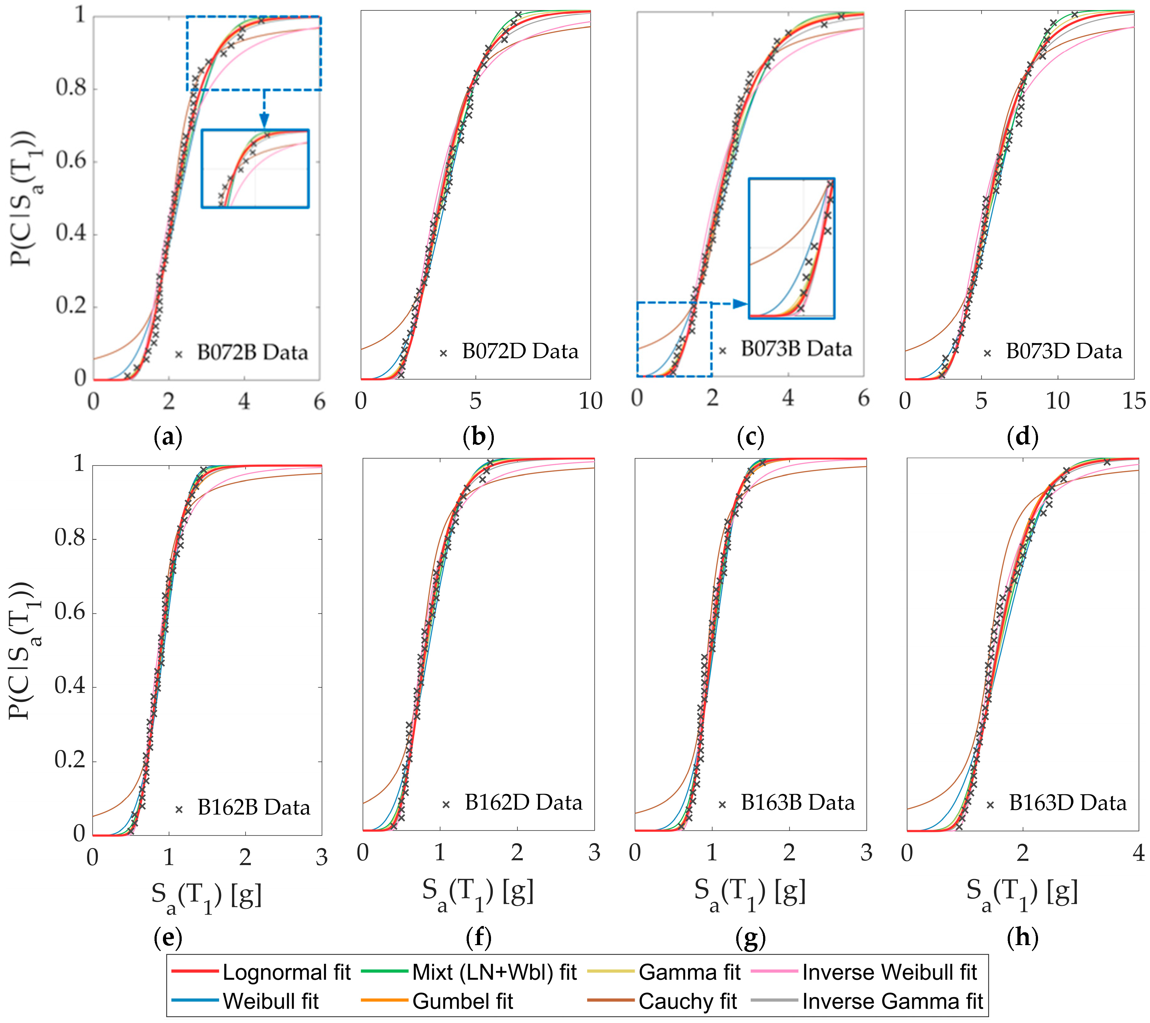
Figure 2 shows the collapse fragility functions of the eight archetypes. It is notable that, at small values of S a ( T 1 ) , the lower tails of some PDFs (mostly the Weibull and Cauchy) are well above the data, whereas at large values of S a ( T 1 ) the upper tails of other PDFs (mostly the Inverse Weibull and Inverse Gamma) are well below the data.
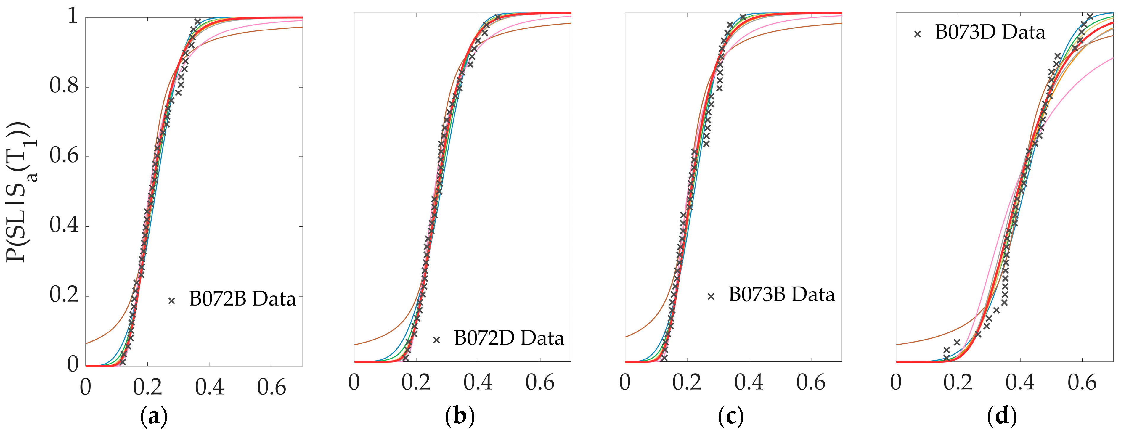
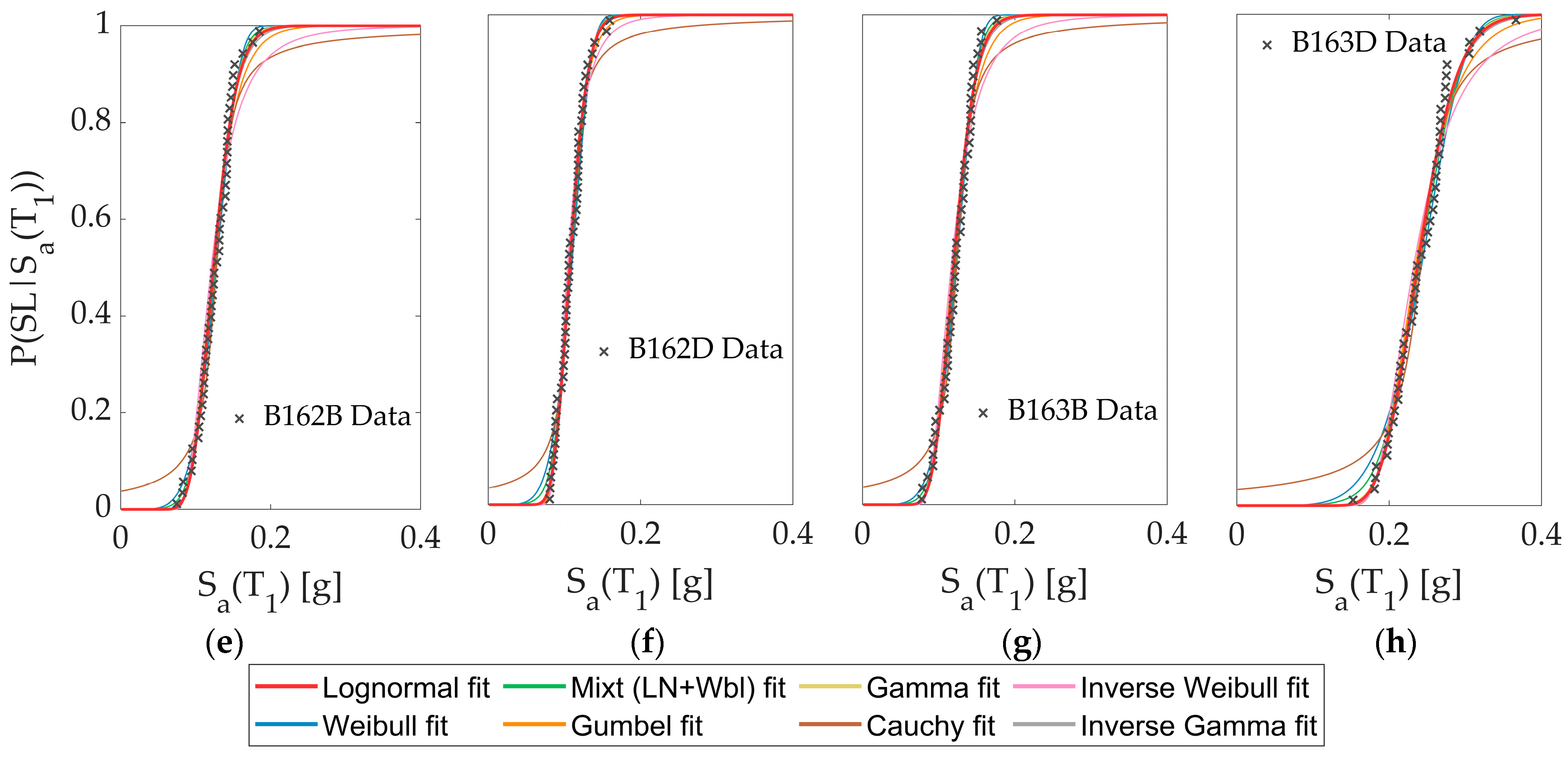
Figure 3 shows the SL fragility functions. Notably, the abovementioned observations on the collapse fragility functions also apply in this case.

3.2. Assessment of the Quality of the Fragility Functions

The procedure is briefly described in FEMA P-58. The objective is to assign a quality level to a fragility function according to the criteria of Table H-5 of FEMA P-58 [4]. In order to obtain high-quality fragility functions, the data must satisfy all the requirements summarized in Table 2.
Table 2 shows that the data used in this study do comply with the requirements of FEMA P-58. In other words, the data are adequate to obtain high-quality fragility functions. Table 2 also shows that, as explained in the next subsections, alternative and more conservative goodness-of-fit tests were also considered in this study, as well as an alternative criterion to identify outliers.

3.2.1. Goodness-of-Fit Tests

The FEMA P-58 methodology suggests that fragility functions should pass a Lilliefors test at a 5% significance level. However, FEMA P-58 also indicates that higher (15%) or lower (2.5%) significance levels are also possible. This study’s most conservative testing criterion (2.5% significance level) was also considered to reduce the probability of a “false negative”. More negligible significance levels minimize the likelihood of rejecting the null hypothesis when true.
Although FEMA P-58 requires the Lilliefors (Lill) test only, alternative methods such as the Kolmogorov–Smirnoff (K–S) and the Anderson–Darling (A–D) tests have also been widely used in PBEE studies. For this reason, both methods are also considered in this section.
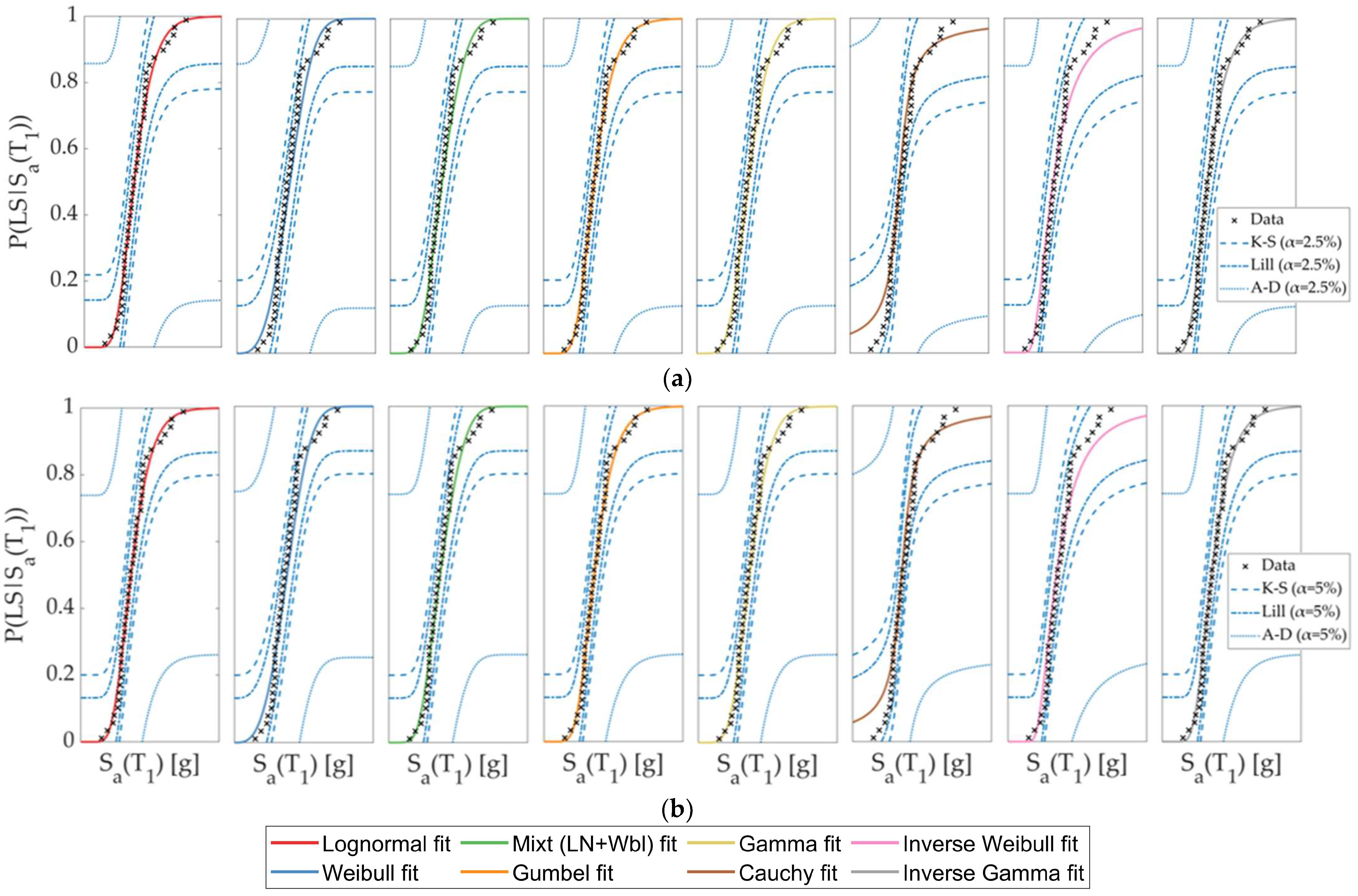
Figure 4 shows the results of all the goodness-of-fit tests (i.e., the Lill., K–S, and A–D methods at both 2.5% and 5% significance levels) applied to the collapse fragility data of archetype B072D. Results for all the other archetypes are qualitatively identical to those shown in Figure 4 and are not offered for brevity.
As seen in Figure 4, the most conservative method is the Lilliefors test, and the most unconservative is the A–D test. It is also observed that all the PDFs pass the goodness-of-fit tests, even at the more conservative 2.5% significance level. Consequently, the quality of the fragility functions is not sensitive to the significance level of either the test proposed by FEMA P-58 (i.e., the Lill) or the other tests considered in this study (i.e., the K–S and A–D tests). Still, these tests might give different results when applied to low-quality data; in such a case, the fragility functions might end up being rejected by the Lill test but being accepted by the A–D test.

3.2.2. Identification of Data Outliers

Data outliers or spurious data may be present when fragility functions are derived from data affected by experimental or numerical errors, [4] because, in such scenarios, each observation is altered by random and systematic errors [43]. It is important to remark that data outliers can significantly impact the value of the estimated parameters of the assumed PDF [43].
Fragility functions, especially in the case of LS, such as collapse, usually exhibit a nonlinear trend, and it is not always evident whether suspicious observations exist or not. Hence, an objective outlier identification criterion is needed to avoid confusion between discordant random observations and suspicious observations [44]. In this context, this study adopts Peirce’s criterion suggested by FEMA P-58 [4] and the leverage criterion proposed in the primary probability literature [44]. Previous studies have suggested both methods for collapse assessment [7].
The FEMA P-58 methodology adopts Peirce’s criterion to detect data outliers in the general case where the quantity of suspicious data is unknown [43]. The iterative procedure to implement Peirce’s criterion is described in detail in FEMA P-58. Even though FEMA P-58 indicates that Peirce’s criterion “should be applied”, it is known that other methods to detect data outliers may or may not give different results. Further, in seismic fragility analysis, the elimination of data outliers at the S a T 1 θ i range is more important than at the S a T 1 > θ i range because IM levels associated with the former are much more frequent than IM levels related to the latter. Therefore, the influence of data outliers at the S a T 1 θ i range on risk metrics is much more important than that of data outliers at the S a T 1 > θ i range.
On the other hand, the leverage criterion quantifies how far away the value of an individual observation is from the others [44]. Thus, the leverage statistic value h i is computed for each ith observation as follows [45]:
h i x i = 1 n + ( x i x ¯ ) 2 i = 1 n ( x i x ¯ ) 2 ,
where x = ln( S a ( T 1 ) ), x ¯ is the mean of the independent variable x, and n is the sample size. A high-leverage observation has an unusual value of x i , which suggests an outlier [8]. The warning threshold suggested for collapse assessment is 2.5 of the average leverage h avg [7].
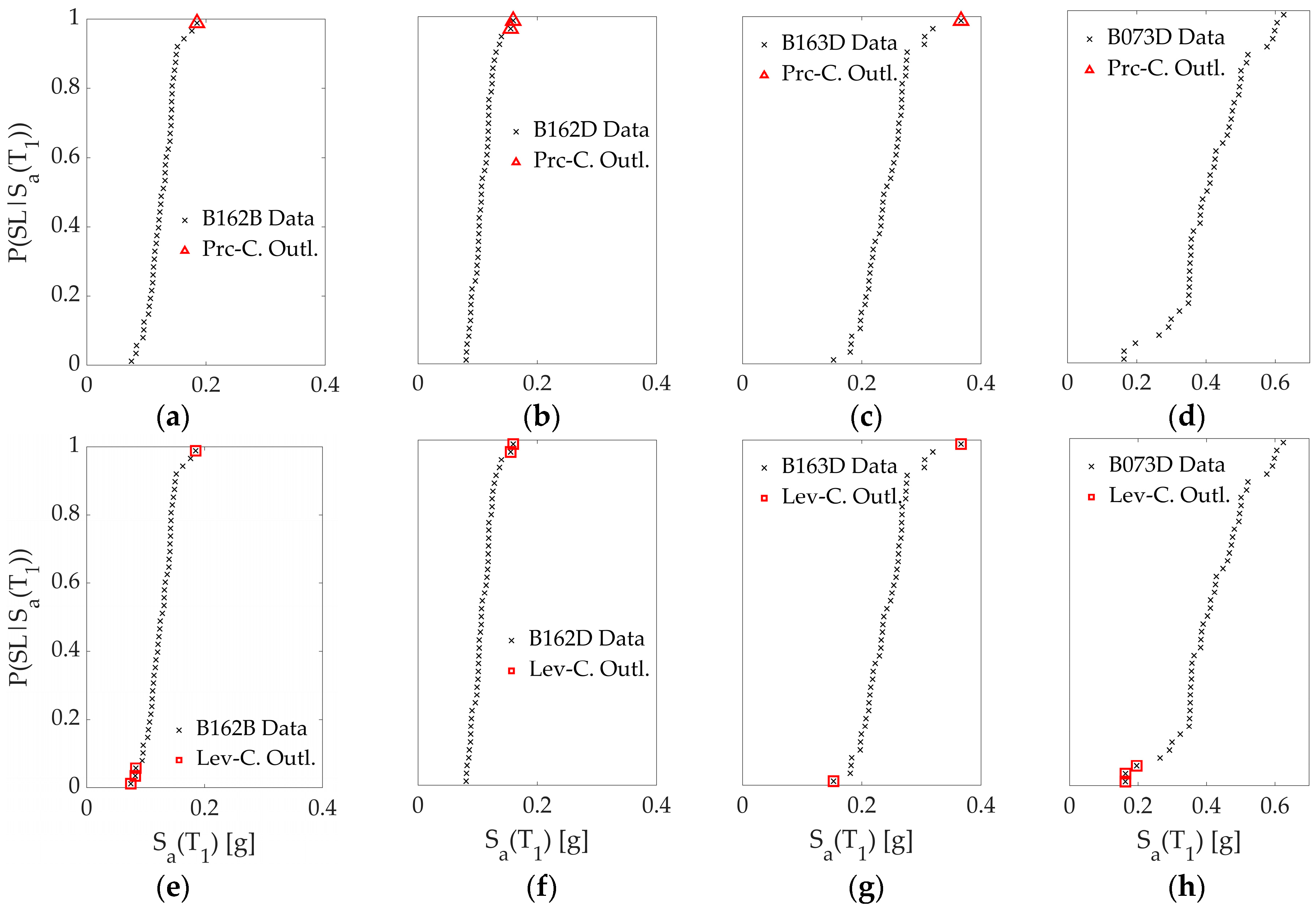
Figure 5 shows the collapse fragility data of those cases (i.e., archetypes) in which data outliers identified by both methods are most significant. Notably, the leverage criterion tends to be more sensitive to suspicious values at the S a T 1 θ i range (i.e., at the lower tail of the fragility functions), whereas Peirce’s criterion tends to be more sensitive to suspicious values at the S a T 1 > θ i range (i.e., at the upper tail of the fragility function). Removing data outliers at the lower tail of the fragility functions usually has a more significant impact on the value of re-estimated parameters and, as already discussed, on risk metrics such as the mean annual frequency of collapse.
Figure 6 shows the SL fragility data of three high-rise archetypes and one mid-rise archetype, together with the data outliers identified by both methods. In general, few data outliers are identified in the SL fragility data of the mid-rise archetypes. More data outliers are identified in the SL fragility data of the high-rise archetypes, but still not as many as in the collapse fragility data. Again, it can be seen that, when applied to the same data set, the two technically valid outlier detection methods (i.e., Peirce’s criterion and the leverage criterion) generally give different results and tend to identify outliers at other parts of the fragility functions (i.e., Peirce’s criterion tends to recognize more outliers at the upper tail of the fragility curve, whereas the leverage criterion tends to identify more outliers at the lower part of the fragility curve).

3.2.3. Comparison of Estimated Parameters

As mentioned before, once the outliers have been removed, it is necessary to re-estimate the parameters of the fragility PDF considering the new data set (i.e., the data that remain after removing the outliers). If any of the revised parameters differ from the original ones by more than 20%, the fragility functions should be modified considering the reviewed parameters. It is worth mentioning, however, that in many PBEE studies, data outliers are not identified and, consequently, not removed (this issue is not even mentioned in such studies).
Table 3 summarizes the differences between the original and reviewed parameters calculated considering the collapse fragility data of the four mid-rise archetypes for which such differences are found most significant. Differences equal to or larger than 20% are marked in red. It can be observed that, in some cases, the difference is substantial (up to 67%). Also, it is interesting to note that, in the case of the Lognormal PDF, the difference is never greater than 20% (regardless of the outlier detection method). However, in just one case (archetype B072B, leverage criterion), the difference between the original and reviewed values of the second parameter is 19.21% (i.e., slightly less than the 20% limit). On the other hand, differences more significant than 20% are more common when the Gamma PDF is adopted.
Table 4 summarizes the differences between the original and reviewed parameters calculated considering the collapse fragility data of the four high-rise archetypes for which such differences are found most significant. The number of cases in which differences are equal to or larger than 20% is less than that in Table 3, and all such cases occur exclusively when the Weibull, Gamma, and Inverse Gamma PDFs are adopted.
Table 5 summarizes the differences between the original and reviewed parameters calculated considering the SL fragility data of the four mid-rise archetypes for which such differences are found most significant. Cases where differences are equal to or larger than 20% are observed only in the fragility of archetype B073D and only when the leverage criterion is applied. It must be noticed that archetype B073D is the one for which the collapse Sa(T1) values are the largest and have a significant degree of dispersion. Further, as shown in Figure 6, the leverage criterion only identified outliers at the lower tail.
Finally, Table 6 summarizes the differences between the original and reviewed parameters calculated considering the SL fragility data of the four high-rise archetypes for which such differences are found most significant. A comparison between Table 5 and Table 6 (i.e., SL fragility) shows that, unlike what is observed in collapse fragility (Table 3 and Table 4), the number of cases in which differences are equal to or larger than 20% is more significant in high-rise buildings than in mid-rise buildings, particularly when the leverage criterion is applied.
In all cases, the value of the estimated logarithmic standard deviation β of the Lognormal PDF is found to comply with the 0.2 ≤ β ≤ 0.6 limits.
According to the FEMA P-58 procedure, fragility functions that exhibit differences equal to or more significant than 20% between original and reviewed parameters do not qualify as high-quality fragility functions. Still, the FEMA P-58 procedure does not explicitly reject such fragility functions (in fact, it does not indicate how to proceed in such a scenario).
It is worth noting that results in Table 3, Table 4, Table 5 and Table 6 do not exhibit a clear correlation between PDFs and the differences between original and reviewed parameters or between PDFs and data outlier detections (regardless of the detection method).

3.2.4. Comparison of Alternative PDFs

In the context of selecting the most adequate statistical model to represent a set of observations (data), information criteria are mathematical tools that provide a value indicating the adequacy of a given model. If different models are considered, an information criterion gives a value for each model [22]. Such values can then be compared, and the model that gives the smallest value is deemed the most suitable [22]. The Akaike Information Criterion (AIC) and the Bayesian Information Criterion (BIC) are commonly used for model selection [46]. The AIC value for a given model “M” with parameter θ M depends on the likelihood L M and the number of the model parameters n p :
AIC = 2 ln L M ( θ M ) + 2 n p
A modification of the AIC equation gives the BIC value to avoid possible over-fitting [47]:
BIC = 2 ln L M ( θ M ) + ln ( N s ) n p
where N s is the sample size.
In this study, these multi-comparative analysis tools are considered to evaluate the fragility functions before and after removing data outliers with both Peirce’s and the leverage criterion.
Table 7 summarizes the results of the multi-comparative analysis of the collapse fragility of the mid-rise archetypes. The PDFs are presented in ascending order from the best (in green) to the worst (in red). In all cases, the Lognormal PDF is highlighted. It is worth noting that the Lognormal PDF is never the worst-rated, but only twice is the best-placed. However, the Gamma PDF is often the best-rated for these archetypes, regardless of whether data outliers have been eliminated or not.
Table 8 summarizes the results of the multi-comparative analysis of the collapse fragility of the high-rise archetypes. Again, the Lognormal PDF is never the worst-rated, but only twice is the best-placed. However, the Inverse Gamma PDF is often the best-rated for these archetypes, regardless of whether data outliers have been eliminated or not.
Similarly, Table 9 indicates the results of the multi-comparative analysis with AIC and BIC for the SL of mid-rise buildings. It is worth mentioning that in this case (mid-rise buildings and SL LS, which is associated with minimal nonlinear behavior and, thus, reduced variability), only the Lev-C. outlier identification criterion detected data outliers in just one case (B073D), therefore, only in this case, the AIC and BIC criteria were subsequently applied to perform a quantitative assessment of how well the alternative PDFs adjust to the data. For the remaining archetypes, data outliers were not identified, and thus, the application of the AIC and BIC criteria was the same with and without the application of the outlier detection methods. In terms of the results, it can be seen that, once more, the Lognormal PDF is never the best-rated.
Finally, Table 10 summarizes the results of the multi-comparative analysis of the SL fragility of the high-rise archetypes. As before, the Lognormal PDF is never the worst-rated. However, the mixture PDF is often the best-placed for these archetypes, regardless of whether data outliers have been eliminated or not.
In 80 out of 82 cases, the Cauchy PDF is, by far, the worst-ranked PDF. This observation may be due to the pronounced s-shaped nature of the Cauchy PDF that does not provide the required positive skewness. However, once the Cauchy PDF is excluded, no PDF appears to be either the best- or the worst-suited for all mid- and high-rise buildings and both LS. This outcome confirms that the analysis presented in this section should be carried out for each fragility assessment instead of assuming a priori a given PDF. However, differences among alternative PDFs are non-negligible for the collapse LS, while for the Service Level LS, these differences are minor. Consequently, given that these types of analyses are computationally very low-cost intensive when compared with other computational methods used in PBEE (e.g., finite element models or IDAs), they could be easily implemented on a case-to-case basis to provide the best fitting to each particular data set and, thus, to obtain more accurate estimations, especially in the case of collapse LS.
According to FEMA P-58, the eight PDFs considered in this study lead to high-quality fragility functions (both collapse and SL) for all the archetypes. However, although they are all equally valid in principle, they might result in significantly different values of risk metrics. This issue is evaluated in the next section.

4. Impact of Alternative Fragility Functions on Annualized Performance-Based Metrics

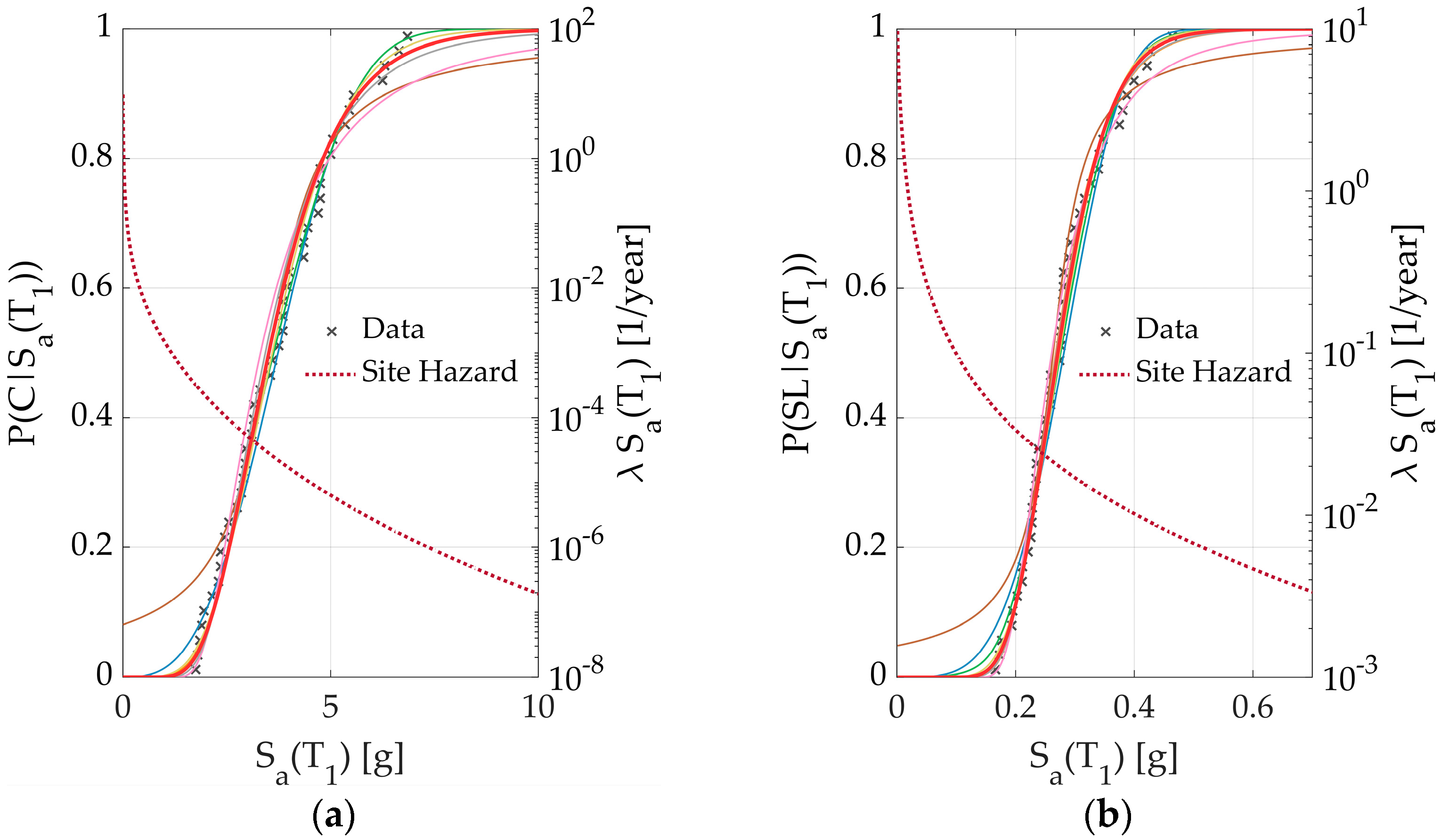
Fragility functions are integrated with their corresponding seismic hazard curves to obtain annualized performance-based metrics, such as the mean annual frequency of collapse ( λ L S ), as indicated in Figure 7. In particular, Figure 7a,b show examples of simulated data, fitted fragility functions (using the same colors defined across this study for each particular PDF), and site hazard curves for collapse LS and SL LS, respectively, for archetype B162B. Figure 7a, associated to collapse LS, shows more considerable data variability than Figure 7b, associated to SL LS, which is reasonable since collapse represents a LS dominated by nonlinear behavior. In contrast, SL LS is usually associated with linear behavior.
Then, the probability for each LS assessment in 50 years is obtained with Equation (12), where all the parameters have been previously defined:
P L S ( 50 ) = 1 e λ L S . 50 ,

Metrics Variability

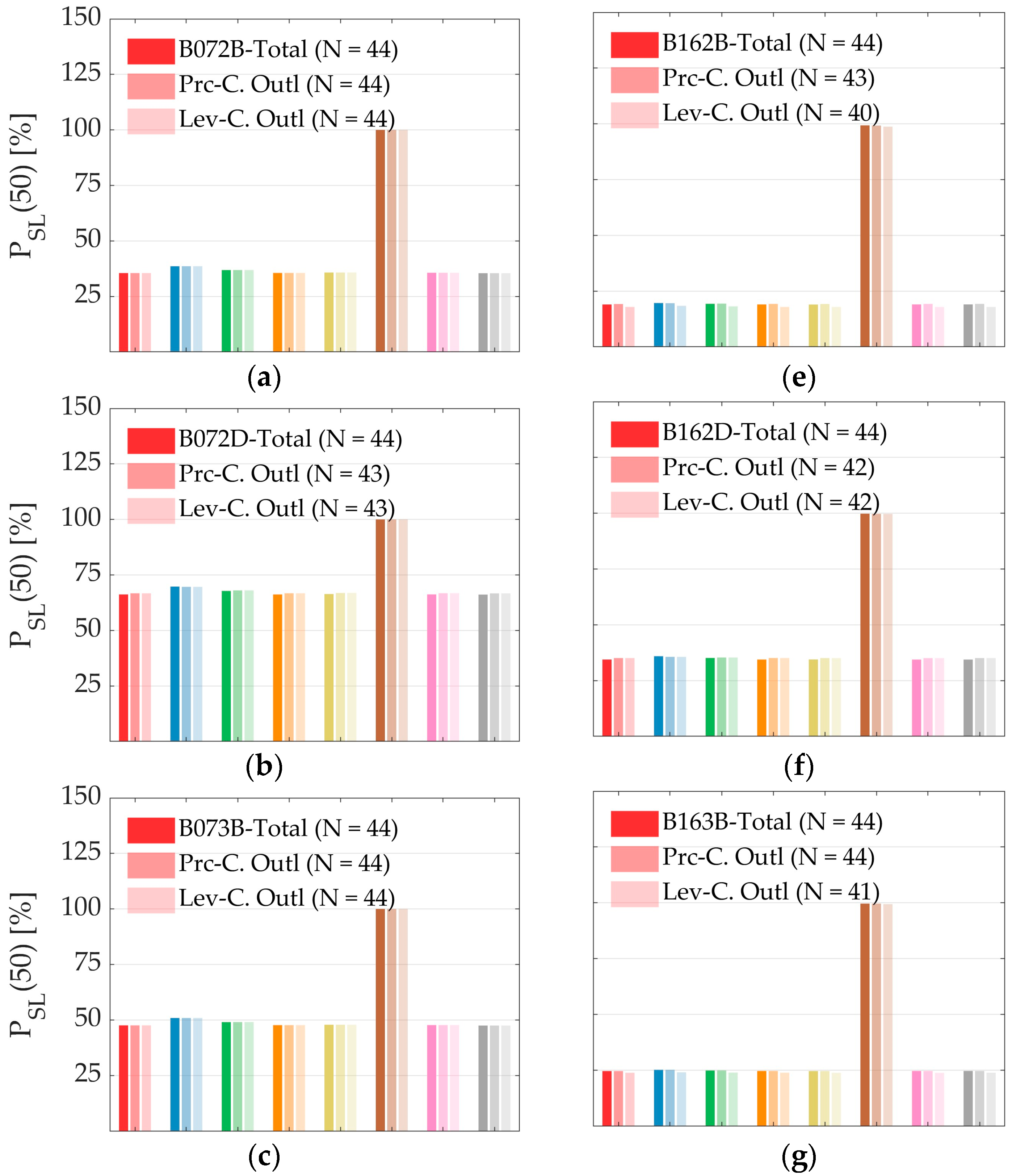
Since eight fragility functions (associated with the eight PDFs used in this study) for each building are developed, and these eight fragility functions are then used (i) without elimination of data outliers; (ii) with elimination of data outliers using Peirce’s criterion; and (iii) with elimination of data outliers using the leverage criteria, a total of 24 values of these metrics are calculated for each LS assessment for each building.
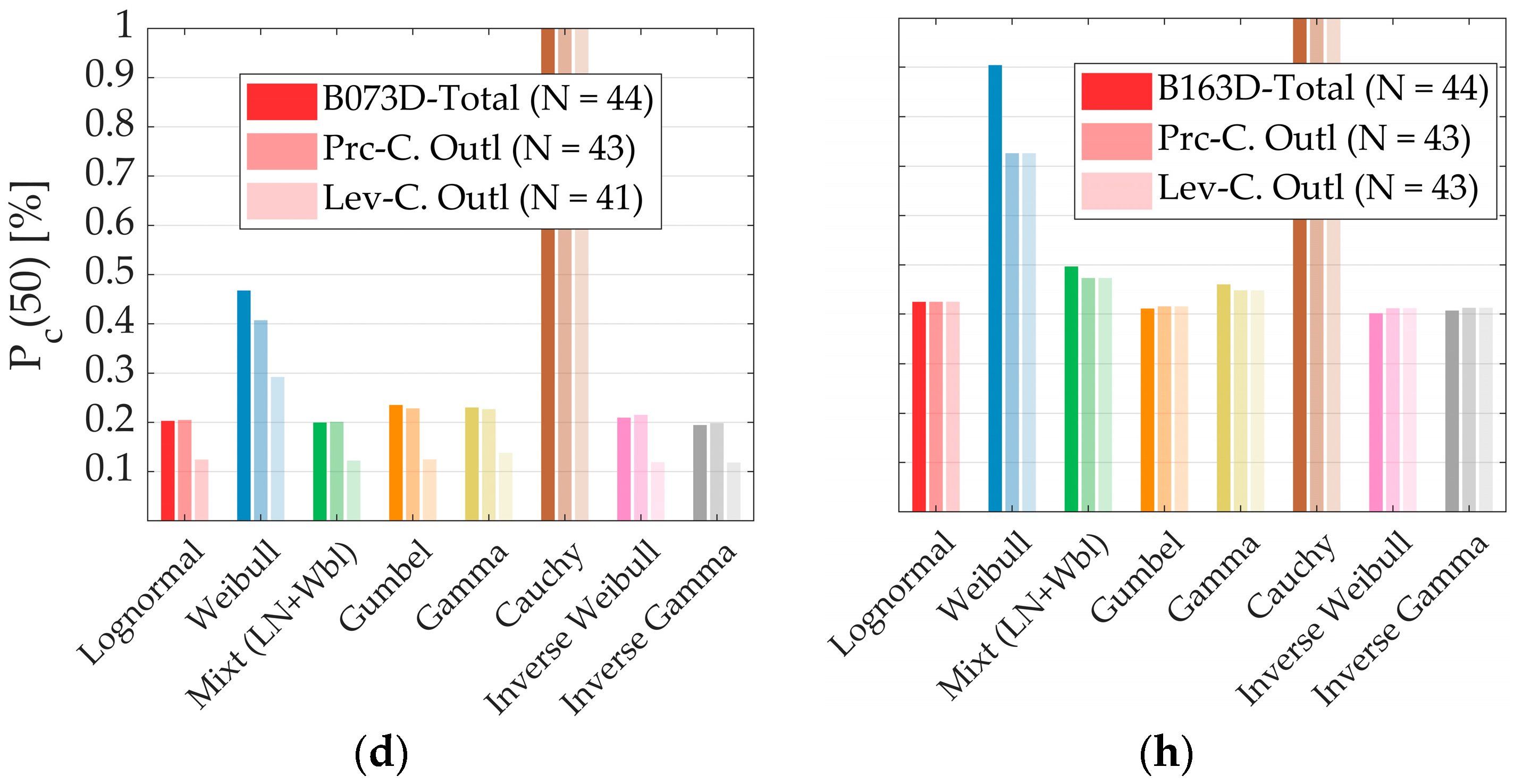
The latter is shown in Figure 8a–h, which depicts the 24 values of the probability of collapse in 50 years, P c ( 50 ) for each of the eight archetype buildings. This figure shows that P c ( 50 ) values are less than 1%, except for the Cauchy PDF, which in all cases is a value of 100%. It is worth mentioning that a target probability of collapse of 1% in 50 years is stated by ASCE 7–22 [48], and both simulation and empirical evidence have shown that code-conforming-designed Chilean buildings, such as the ones used in this study, overall meet this limit of 1%. Consequently, the range of Figure 8 has been limited to 1%, and since the calculated P c ( 50 ) values obtained by Cauchy PDF are inconsistent with both simulation and empirical evidence, this PDF is not considered for further analyses.
Excluding the Cauchy PDF, Figure 8 presents significant variability in their P c ( 50 ) values across different buildings (which is expected since these buildings are designed following the Chilean seismic design code, which is a prescriptive code not intended to estimate nor provide a uniform collapse performance). For all buildings, it is evident that the application of Weibull PDFs to obtain fragility functions leads to the maximum P c ( 50 ) values and the remaining PDFs tend to calculate close P c ( 50 ) values between them. Consequently, the difference between the values obtained with the Weibull PDF and other PDF is significant and should be carefully analyzed. For the extreme case corresponding to building B073B, note that the value obtained with the Weibull PDF is 2.82 times that obtained with the Lognormal PDF, considering all data (without eliminating outliers). Therefore, for the collapse LS, it is suggested to consider alternative PDFs and carry out the multi-comparative analysis for model-selection assessment. In terms of the impact of the outlier detection methods, it can be seen that, in general, the application of these methods tends to reduce the obtained P c ( 50 ) values (there are some exceptions, such as archetype B162D, where Lognormal, Gumbel, and Inverse Weibull PDFs lead to slightly larger P c ( 50 ) values when outliers are removed). The latter results can be explained since outliers are usually located at the upper tail in the case of collapse LS and, thus, elimination of these extreme values leads to fragility functions shifted to the left and, consequently, smaller P c ( 50 ) values.
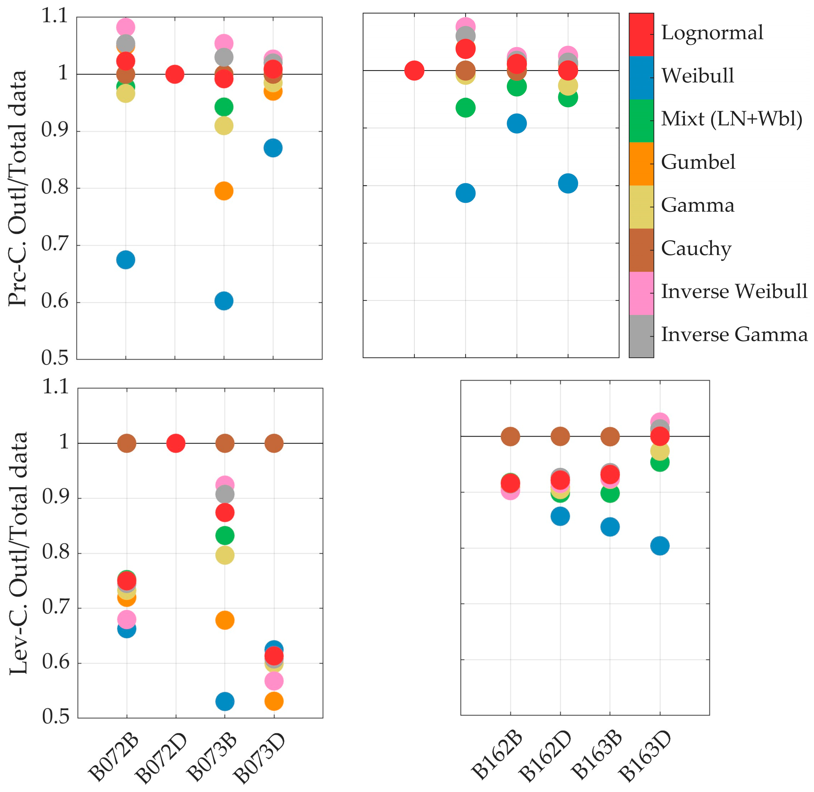
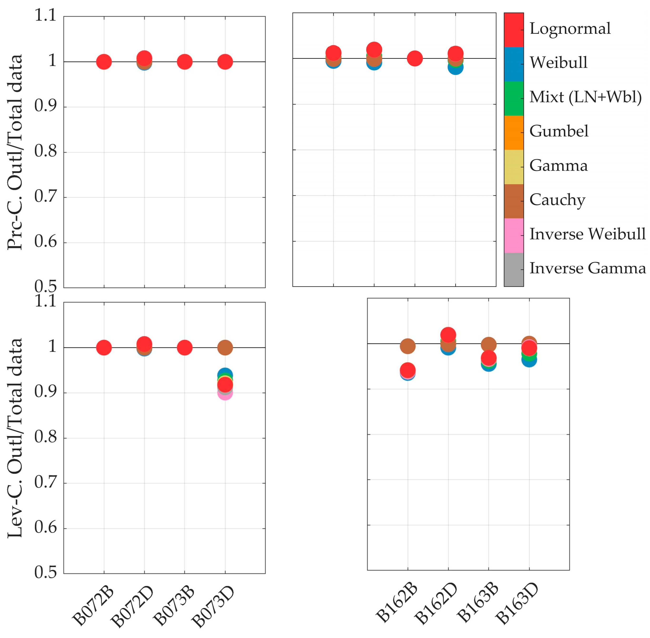
In addition, Figure 9 shows the rates of the P c ( 50 ) obtained with the fragility functions after the elimination of data outliers detected with Peirce’s and leverage criteria and the P c 50 obtained with all the data. As seen in this figure, significant differences can be obtained in annualized terms, especially for the Weibull PDFs, where usually the P c ( 50 ) obtained without the elimination of outliers is more significant than the values obtained once outliers have been removed (since, as mentioned before, usually those outliers are located at the upper tail of the fragility functions). For instance, in the case of the archetype B073B and the use of the Weibull PDF, the ratio between P c 50 values obtained with the leverage criterion, and the total data are as small as 0.52.
On the other hand, Figure 10 indicates the probabilities of reaching the SL LS in a 50-year time frame, P S L ( 50 ) , for mid-rise and high-rise buildings. These results indicate that, except for the Cauchy PDF, there is negligible variability in the outcomes obtained with alternative PDFs. This fact is explained because, for SL LS, the structure remains essentially elastic or has very few incursions of nonlinearities. It is important to remark that the Cauchy distribution is the worst-ranked PDF in the previous multi-comparative analysis, and the value of 100% obtained with this PDF for P S L ( 50 ) is not consistent with both simulated and empirical data. Since the use and evaluation of alternative PDFs have a significantly lower impact on the SL LS compared with the collapse LS, the step of the multi-comparative analysis for model-selection assessment could be skipped.
Moreover, Figure 11 depicts the rates of the P S L ( 50 ) obtained with the fragility functions after the elimination of data outliers detected with Peirce’s and leverage criteria and the P S L 50 obtained with all the data. As expected, since SL is a limit state before collapse (presenting significantly less nonlinear behavior and, thus, less variability than collapse), the differences between fragilities, in annualized terms, before and after outlier removal are especially more minor, indicating that the PDF selection in this previous LS is significantly less sensitive than in collapse LS.

5. Conclusions

This study evaluates the numerical impacts of selecting different probabilistic models (isolated or in combination) on the estimation of seismic risk metrics via the generation of fragility functions and also their integration with their respective seismic hazard curves for a set of eight Reinforced Concrete (RC) dual wall–frame buildings, whose seismic performance simulated data have been previously obtained using incremental dynamic analyses. Specifically, alternative (and technically valid) probabilistic models are implemented and evaluated for (i) the identification and elimination/replacement of unusual observations (i.e., outliers) within the simulated data; (ii) the selection and implementation of different Probability Distribution Functions (PDFs) to estimate fragility functions for different Limit States (LS); and (iii) the application of goodness-of-fit tests as well as information criteria to evaluate the agreement between the proposed fragility functions and the simulated data. Based on the results, the following conclusions can be drawn towards the analyses and design of more resilient and sustainable built environments:
  • Even though the Lognormal PDF is, by far, the most widely used PDF within Performance-Based Earthquake Engineering (PBEE), there are other PDFs, such as Weibull or Gamma, that are technically valid (e.g., positive-skewed distribution) to represent fragility functions, that pass goodness-of-fit tests, but that provide significantly different adjustments in some part of the fragility functions (e.g., the Lognormal PDF usually adjusts better to the data in the lower part of the fragility function, whereas the Weibull PDF often adjusts better to the data in the upper part of the fragility function. Actually, a Lognormal PDF is not always the best representation of the data).
  • Even though the simulated data used in this study passed all alternative goodness-of-fit tests, the Lilliefors test always resulted in the stricter test for the same confidence level when compared with the Kolmogorov–Smirnov (K–S) and Anderson–Darling (A–D) tests. It is worth noting that several studies have addressed PBEE use of the K–S, which is a more relaxed test that might lead to fragility functions that the Lilliefors test could have rejected.
  • Nevertheless, the use of outlier detection methods to remove unusual data and the subsequent estimation of new parameters (when the difference between previous and posterior parameters differs by more than 20%) is recommended by FEMA P-58; several studies within PBEE do not even mention the application of this process. In this study, several PDFs presented differences larger than 20% (never the Lognormal PDF, but still showed a −19.21% difference in one case), highlighting the need to implement these outlier detection methods. When comparing past and new estimated parameters after the elimination of data outliers, there is no correlation between which PDF is the one that exhibits the lower or higher variability. This variability is also not explained by a correlation between the leverage or Peirce’s criteria.
  • The leverage criterion tends to be more sensitive to the suspicious data of the lower tails of the fragility functions. In contrast, Peirce’s criterion tends to be more sensitive to the upper tail of the fragility functions. The latter effects might generate significant differences, since lower values (located at the lower tail of the fragility functions) tend to affect more annualized metrics associated with intensity measures that occur more often. The latter explains why applying the leverage criterion exhibits the most variability in the assessment measures.
  • The use of information criteria allows the quantitative evaluation of alternative PDF based on their adjustment to data, and there is no correlation between best-ranked fitted functions for the eight buildings used in this study. In particular, the Cauchy PDF is always the worst function. At the same time, the Inverse Gamma and Inverse Weibull usually fit better after eliminating the data outlier for the case of collapse LS. However, the Mixture PDF proposed in this study (a combination of a Lognormal PDF and Weibull PDF from 0 to 50% and from 50% to 100%, respectively) tends to fit better for mid-rise RC buildings for Service-Level LS.
  • Finally, it is essential to highlight that even though there have been several efforts to advance to more accurate experimental and numerical methods within PBEE to better predict the performance of our built environment (in terms of casualties, environmental impacts, economic losses, and downtime) fewer efforts have been placed on assessing alternative probabilistic methods, whose impacts can be even more significant than some differences generated by some, for instance, structural modeling methods. Consequently, this study recommends the use of multi-comparative analyses for probabilistic model selection (including the alternative outlier detection methods, the PDFs, and the information criteria analyses proposed in this study, except the Cauchy PDF) on a case-to-case basis for extreme LS, such as collapse. These extreme LSs are characterized by large variability (high nonlinear behavior), and significant differences are detected when applying alternative probabilistic methods. Thus, the implementation of these computationally very low-cost intensive probabilistic methods, when compared with other computational methods used in PBEE (e.g., finite element models or IDAs), is recommended to provide the best fitting to each particular building-specific data set to obtain more accurate PBEE estimations. In the case of the SL LS, since the differences obtained from applying these alternative probabilistic methods have significantly lower impacts, the step of multi-comparative analysis for model-selection assessment could be skipped compared with the collapse LS.

Author Contributions

Conceptualization, M.F.G., G.A.-L. and D.L.-G.; methodology, I.M., M.F.G., G.A.-L. and D.L.-G.; software, I.M. and M.F.G.; validation, M.F.G., G.A.-L. and D.L.-G.; formal analysis, I.M., M.F.G., G.A.-L. and D.L.-G.; investigation, I.M., M.F.G., G.A.-L. and D.L.-G.; resources, G.A.-L. and D.L.-G.; data curation, M.F.G.; writing—original draft preparation, I.M. and M.F.G.; writing—review and editing, G.A.-L. and D.L.-G.; visualization, I.M. and M.F.G.; supervision, G.A.-L. and D.L.-G.; project administration, G.A.-L.; funding acquisition, G.A.-L. All authors have read and agreed to the published version of the manuscript.

Funding

This research was funded by Agencia Nacional de Investigación y Desarrollo(ANID) de Chile, ANID Doctorado Nacional 2018 Folio 21181157, ANID FONDECYT de Iniciación, Grant 11191194, and the Research Center for Integrated Disaster Risk Management (CIGIDEN) ANID FONDAP 1522A0005.

Institutional Review Board Statement

Not applicable.

Informed Consent Statement

Not applicable.

Data Availability Statement

Data are available upon reasonable request.

Acknowledgments

The strong motion database for the IDAs was provided by the SIBER-RISK (Simulation-Based Earthquake Risk and Resilience of Interdependent Systems and Networks) project. Valuable comments on statistical issues were supplied by Darlin Soto, at the Universidad del Bío-Bío. The funding for this article processing charge (APC) was provided by ANID FONDECYT de Iniciación, Grant 11191194, and this support is greatly appreciated.

Conflicts of Interest

The authors declare no conflicts of interest. The funders had no role in the study’s design; in the collection, analyses, or interpretation of data, in the writing of the manuscript, or in the decision to publish the results.

Abbreviations

A–DAnderson–Darling
AICAkaike Information Criteria
BICBayesian Information Criteria
B072B7-story building located in seismic zone 2 on soil type B
B072D7-story building located in seismic zone 2 on soil type D
B073B7-story building located in seismic zone 3 on soil type B
B073D7-story building located in seismic zone 3 on soil type D
B162B16-story building located in seismic zone 2 on soil type B
B162D16-story building located in seismic zone 2 on soil type D
B163B16-story building located in seismic zone 3 on soil type B
B163D16-story building located in seismic zone 3 on soil type D
CDFCumulative Distribution Function
DSDamage State
EDPEngineering Demand Parameter
IDAIncremental Dynamic Analysis
IMIntensity Measure
K–SKolmogorov–Smirnov goodness-of-fit test
Lev-C.Leverage criterion for data outlier
Lill.Lilliefors goodness-of-fit test
LSLimit State
MLMMaximum Likelihood Method
SLService Level
PBEEPerformance-Based Earthquake Engineering
Prc-C.Peirce’s criterion for data outlier
PDFProbability Distribution Function
PFAPeak Floor Acceleration
PSDRPeak Story Drift Ratio
RCReinforced Concrete
RDRRoof Drift Ratio
Notation list
S a ( T 1 ) Spectral acceleration ordinate at the fundamental period of the structure
P LS S a ( T 1 ) Probability of a specific limit state conditioned on the spectral pseudo acceleration
λ LS Mean annual frequency of a specific limit state
P LS ( 50 ) Probability of exceeding a specific limit state in a time of 50 years

References

  1. Krawinkler, H.; Miranda, E. Performance-Based Earthquake Engineering. In Earthquake Engineering: From Engineering Seismology to Performance-Based Engineering; Bozorgnia, Y., Bertero, V.V., Eds.; CRC Press: Boca Raton, FL, USA, 2004. [Google Scholar]
  2. Deierlein, G.G. Overview of a Comprehensive Framework for Earthquake Performance Assessment. In Proceedings of the International Workshop on Performance-Based Seismic Design—Concepts and Implementation, Bled, Slovenia, 28 June–1 July 2004; pp. 15–26. [Google Scholar]
  3. Özsoy Özbay, A.E. A Decision Tree-Based Damage Estimation Approach for Preliminary Seismic Assessment of Reinforced Concrete Buildings. Rev. De La Construcción 2023, 22, 5–15. [Google Scholar] [CrossRef]
  4. FEMA (Federal Emergency Management Agency). Seismic Performance Assessment of Buildings; FEMA P-58-1; FEMA: Washington, DC, USA, 2018.
  5. Calderón, S.; Vargas, L.; Sandoval, C.; Araya-Letelier, G.; Milani, G. Shear Design Equation and Updated Fragility Functions for Partially Grouted Reinforced Masonry Shear Walls. J. Build. Eng. 2022, 50, 104097. [Google Scholar] [CrossRef]
  6. Zhang, Z.; Murcia-Delso, J.; Sandoval, C.; Araya-Letelier, G.; Wang, F. In-Plane Shear Strength and Damage Fragility Functions for Partially-Grouted Reinforced Masonry Walls with Bond-Beam Reinforcement. Eng. Struct. 2021, 242, 112569. [Google Scholar] [CrossRef]
  7. Gallegos, M.; Araya-Letelier, G.; Lopez-Garcia, D. Influence of statistical approaches on structural collapse potential assessment. In Proceedings of the 12th National Conference in Earthquake Engineering, Salt Lake City, UT, USA, 27 June–1 July 2022; Earthquake Engineering Research Institute: Salt Lake City, UT, USA, 2022. [Google Scholar]
  8. Araya-Letelier, G.; Parra, P.F.; Lopez-Garcia, D.; Garcia-Valdes, A.; Candia, G.; Lagos, R. Collapse Risk Assessment of a Chilean Dual Wall-Frame Reinforced Concrete Office Building. Eng. Struct. 2019, 183, 770–779. [Google Scholar] [CrossRef]
  9. Pan, J.-X.; Fang, K.-T. Maximum Likelihood Estimation. In Growth Curve Models and Statistical Diagnostics; Pan, J.-X., Fang, K.-T., Eds.; Springer: New York, NY, USA, 2002; pp. 77–158. [Google Scholar]
  10. Lilliefors, H.W. On the Kolmogorov–Smirnov Test for Normality with Mean and Variance Unknown. J. Am. Stat. Assoc. 1967, 62, 399–402. [Google Scholar] [CrossRef]
  11. Massey, F.J. The Kolmogorov–Smirnov Test for Goodness of Fit. J. Am. Stat. Assoc. 1951, 46, 68–78. [Google Scholar] [CrossRef]
  12. Ruggieri, S.; Calò, M.; Cardellicchio, A.; Uva, G. Analytical-Mechanical Based Framework for Seismic Overall Fragility Analysis of Existing RC Buildings in Town Compartments. Bull. Earthq. Eng. 2022, 20, 8179–8216. [Google Scholar] [CrossRef]
  13. Ruggieri, S.; Liguori, F.S.; Leggieri, V.; Bilotta, A.; Madeo, A.; Casolo, S.; Uva, G. An Archetype-Based Automated Procedure to Derive Global-Local Seismic Fragility of Masonry Building Aggregates: META-FORMA-XL. Int. J. Disaster Risk Reduct. 2023, 95, 103903. [Google Scholar] [CrossRef]
  14. Devore, J. Probability and Statistics for Engineering and the Sciences, 9th ed.; Cengage Learning: San Luis Obispo, CA, USA, 2014. [Google Scholar]
  15. Ibarra, L. Global Collapse of Frame Structures under Seismic Excitations. Ph.D. Thesis, Stanford University, Stanford, CA, USA, 2003. [Google Scholar]
  16. Shome, N. Probabilistic Seismic Demand Analysis of Nonlinear Structures. Ph.D. Thesis, Stanford University, Stanford, CA, USA, 1999. [Google Scholar]
  17. Song, J. Seismic Reliability Evaluation of Steel Frames with Damaged Welded Connections. Ph.D. Thesis, The Johns Hopkins University, Baltimore, MD, USA, 1998. [Google Scholar]
  18. Araya-Letelier, G.; Calderón, S.; Sandoval, C.; Sanhueza, M.; Murcia-Delso, J. Fragility Functions for Partially-Grouted Masonry Shear Walls with Bed-Joint Reinforcement. Eng. Struct. 2019, 191, 206–218. [Google Scholar] [CrossRef]
  19. Ermeydan, I.; Akgönen, A.İ. Investigation on Behavior and Seismic Performance of Reduced Beam Sections. Rev. De La Construcción 2022, 21, 427–446. [Google Scholar] [CrossRef]
  20. Sayin, B.; Cosgun, T.; Gunes, B. A Methodological Approach for Seismic Performance of Existing Single-Storey Industrial RC Precast Facilities. Rev. De La Construcción 2022, 21, 167–183. [Google Scholar] [CrossRef]
  21. Baker, J.; Bradley, B.; Stafford, P. Seismic Hazard and Risk Analysis; Cambridge University Press: Cambridge, UK, 2021. [Google Scholar]
  22. Alfredo, H.S.-A.; Tang, W.H. Probability Concepts in Engineering Planning and Design; John Wiley & Sons. Inc.: New York, NY, USA, 2006; Volume 2. [Google Scholar]
  23. Luko, S.N. A Review of the Weibull Distribution and Selected Engineering Applications. J. Commer. Veh. 1999, 15, 398–412. [Google Scholar]
  24. Ghanaat, Y.; Patev, R.; Chudgar, A. Seismic Fragility Analysis of Concrete Gravity Dams. In Proceedings of the 15th World Conference on Earthquake Engineering, Lisbon, Portugal, 24–28 September 2012; pp. 24–28. [Google Scholar]
  25. Yahyaabadi, A.; Talebkhah, R.; Adibi, M. Development of Seismic Fragility Curves for Precast Concrete Frames with Cast-in-Situ Concrete Shear-Walls. Earthq. Eng. Eng. Vib. 2022, 21, 149–167. [Google Scholar] [CrossRef]
  26. Mandal, T.K.; Ghosh, S.; Pujari, N.N. Seismic Fragility Analysis of a Typical Indian PHWR Containment: Comparison of Fragility Models. Struct. Saf. 2016, 58, 11–19. [Google Scholar] [CrossRef]
  27. Keller, A.Z.; Giblin, M.T.; Farnworth, N.R. Reliability Analysis of Commercial Vehicle Engines. Reliab. Eng. 1985, 10, 15–25. [Google Scholar] [CrossRef]
  28. Mann, N.R. Simplified Expressions for Obtaining Approximately Optimum System- Reliability Confidence Bounds from Exponential Subsystem Data. J. Am. Stat. Assoc. 1974, 69, 492. [Google Scholar]
  29. Fisher, R.A.; Tippett, L.H.C. Limiting Forms of the Frequency Distribution of the Largest or Smallest Member of a Sample. Math. Proc. Camb. Philos. Soc. 1928, 24, 180–190. [Google Scholar] [CrossRef]
  30. Jazi, M.A.; Lai, C.-D.; Alamatsaz, M.H. A Discrete Inverse Weibull Distribution and Estimation of Its Parameters. Stat. Methodol. 2010, 7, 121–132. [Google Scholar] [CrossRef]
  31. Furman, E.; Zitikis, R. A Monotonicity Property of the Composition of Regularized and Inverted-Regularized Gamma Functions with Applications. J. Math. Anal. Appl. 2008, 348, 971–976. [Google Scholar] [CrossRef]
  32. Pedersen, H.L. Inverses of Gamma Functions. Constr. Approx. 2015, 41, 251–267. [Google Scholar] [CrossRef]
  33. Gallegos, M.F.; Araya-Letelier, G.; Lopez-Garcia, D.; Parra, P.F. Collapse Assessment of Mid-Rise RC Dual Wall-Frame Buildings Subjected to Subduction Earthquakes. Buildings 2023, 13, 880. [Google Scholar] [CrossRef]
  34. Gallegos, M.F.; Araya-Letelier, G.; Lopez-Garcia, D.; Parra, P.F. Seismic Collapse Performance of High-Rise RC Dual System Buildings in Subduction Zones. Case Stud. Constr. Mater. 2023, 18, e02042. [Google Scholar] [CrossRef]
  35. NCh433:1996 Mod 2009; INN Norma Chilena Oficial NCh433 Of. 1996 Mod. 2009 Diseño Sismico de Edificios. Instituto Nacional de Normalización: Santiago, Chile, 2009.
  36. MINVU DS 61—Diseño Sismico de Edificios; Ministerio de Vivienda y Urbanismo: Santiago, Chile, 2011.
  37. Vose, D. Risk Analysis, a Quantitative Guide, 3rd ed.; John Wiley & Sons, Ltd.: Chischester, UK, 2000. [Google Scholar]
  38. Baker, J.W. Efficient Analytical Fragility Function Fitting Using Dynamic Structural Analysis. Earthq. Spectra 2015, 31, 579–599. [Google Scholar] [CrossRef]
  39. Cunnane, C. Unbiased Plotting Positions—A Review. J. Hydrol. (Amst.) 1978, 37, 205–222. [Google Scholar] [CrossRef]
  40. Araya-Letelier, G. Design of Building Structural Systems and Enhanced Partition Walls to Improve Life Cycle Costs Associated with Risk of Earthquake Damage. Ph.D. Thesis, Stanford University, Stanford, CA, USA, 2014. [Google Scholar]
  41. Campbell, N.A. Mixture Models and Atypical Values. J. Int. Assoc. Math. Geol. 1984, 16, 465–477. [Google Scholar] [CrossRef]
  42. Albabtain, A.A.; Shrahili, M.; Al-Shehri, M.A.; Kayid, M. Stochastic Comparisons of Weighted Distributions and Their Mixtures. Entropy 2020, 22, 843. [Google Scholar] [CrossRef] [PubMed]
  43. Ross, S.M. Peirce’s Criterion for the Elimination of Suspect Experimental Data. J. Eng. Technol. 2003. Available online: https://classes.engineering.wustl.edu/2009/fall/che473/handouts/OutlierRejection.pdf (accessed on 9 February 2024).
  44. Lglewicz, B.; Hoaglin, D.C. How to Detect and Handle Outliers; Mykytka, E.F., Ed.; American Society for Quality Control, Statistics Division: Milwaukee, WI, USA, 1993; Volume 16. [Google Scholar]
  45. James, G.; Witten, D.; Hastie, T.; Tibshirani, R. An Introduction to Statistical Learning; Springer New York: New York, NY, USA, 2013; Volume 103. [Google Scholar]
  46. Zentner, I. A General Framework for the Estimation of Analytical Fragility Functions Based on Multivariate Probability Distributions. Struct. Saf. 2017, 64, 54–61. [Google Scholar] [CrossRef]
  47. Schwarz, G. Estimating the Dimension of a Model. Ann. Stat. 1978, 2, 461–464. [Google Scholar] [CrossRef]
  48. ASCE (American Association of Civil Engineers). Minimum Design Loads and Associated Criteria for Buildings and Other Structures ASCE/SEI 7-22; American Association of Civil Engineers: Reston, VA, USA, 2022. [Google Scholar]
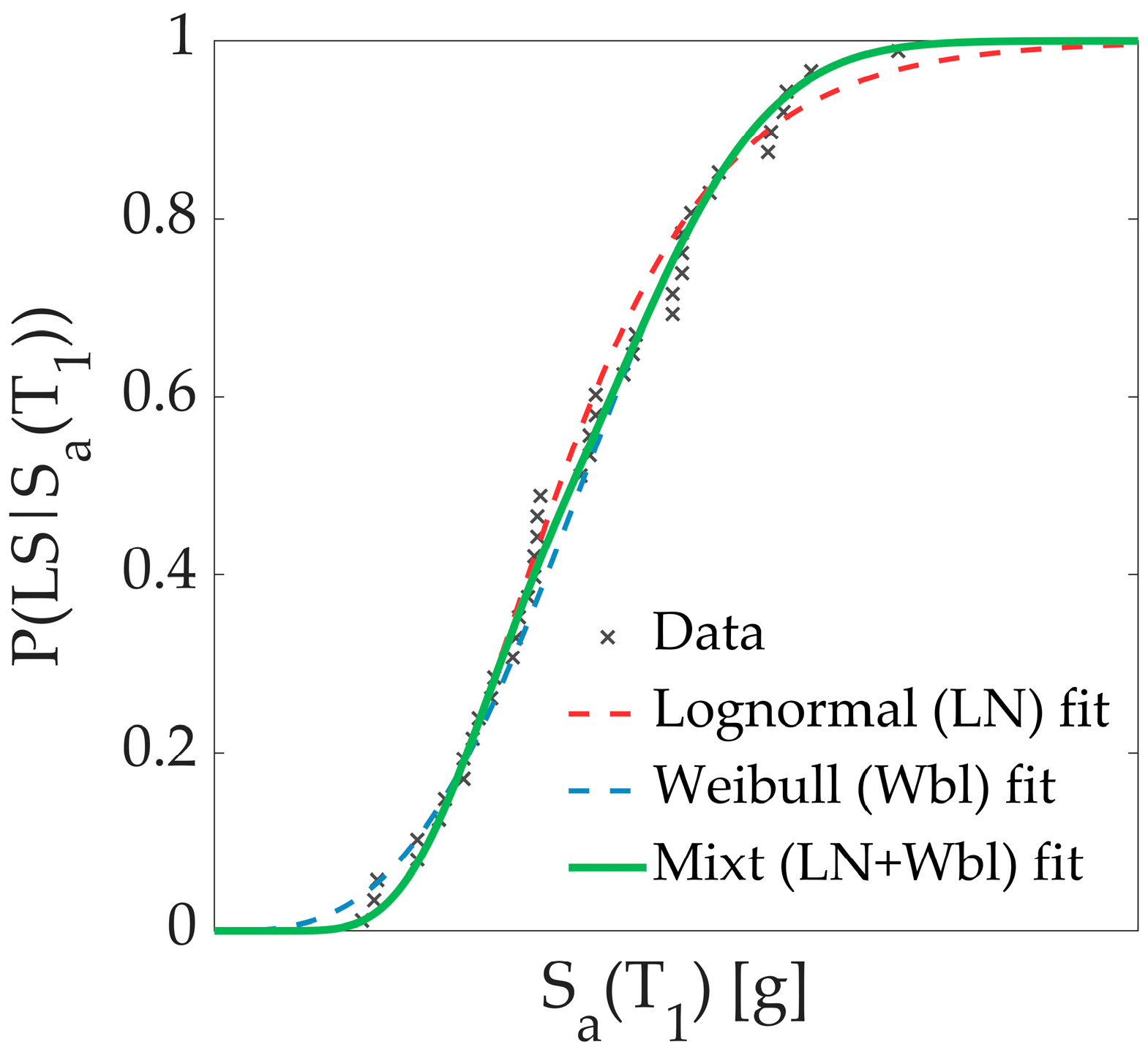
Figure 1. Example of the innovative mixture PDF that is proposed in this study.
Sustainability 16 01668 g001
Figure 2. Collapse fragility functions: (a) B072B, (b) B072D, (c) B073B, (d) B073D, (e) B162B, (f) B162D, (g) B163B, (h) B163D. The simulated data presented in each figure (black crosses) were obtained from [33,34].
Sustainability 16 01668 g002
Figure 3. SL fragility functions: (a) B072B, (b) B072D, (c) B073B, (d) B073D, (e) B162B, (f) B162D, (g) B163B, (h) B163D. The simulated data presented in each figure (black crosses) were obtained from [33,34].
Sustainability 16 01668 g003aSustainability 16 01668 g003b
Figure 4. Goodness-of-fit tests at (a) 2.5% and (b) 5% significance levels (archetype B072D, collapse fragility).
Sustainability 16 01668 g004
Figure 5. Data outlier identification in collapse fragility functions: (a) B072B, (b) B073D, (c) B162D, and (d) B163B (Peirce’s criterion) and (e) B072B, (f) B073D, (g) B162D, and (h) B163B (leverage criterion).
Sustainability 16 01668 g005aSustainability 16 01668 g005b
Figure 6. Data outlier identification SL fragility functions: (a) B072B, (b) B073D, (c) B162D, and (d) B163B (Peirce’s criterion) and (e) B072B, (f) B073D, (g) B162D, and (h) B163B (leverage criterion).
Sustainability 16 01668 g006
Figure 7. Fragility functions integrated with their corresponding site hazard curve (archetype B162B) for the case of (a) collapse LS and (b) SL LS.
Sustainability 16 01668 g007
Figure 8. Comparison of Pc(50) values obtained varying PDFs and use of outlier detection process for archetypes: (a) B072B, (b) B072D, (c) B073B, (d) B073D, (e) B162B, (f) B162D, (g) B163B, (h) B163D.
Sustainability 16 01668 g008aSustainability 16 01668 g008b
Figure 9. The rate between Pc(50) values is obtained after eliminating the data outlier and considering all data (simulations).
Sustainability 16 01668 g009
Figure 10. Variability of PSL(50) for each archetype building: (a) B072B, (b) B072D, (c) B073B, (d) B073D, (e) B162B, (f) B162D, (g) B163B, (h) B163D.
Sustainability 16 01668 g010aSustainability 16 01668 g010b
Figure 11. Rate between PSL(50) obtained after eliminating data outlier and considering all data (simulations).
Sustainability 16 01668 g011
Table 1. Summary of the PDFs considered in this study.
NamePDF1st Parameter2nd ParameterEquation
Lognormal ✓ P ( D S d s i S a T 1 = x = Φ l n ( x / θ i ) β i θ i = median β i = logarithmic standard deviation(1)
Weibull ✓ P ( D S d s i S a T 1 = x = 1 e x / b i a i a i = shape b i = scale(2)
Gumbel ✓ P ( D S d s i S a T 1 = x = e x p e ( x μ i ) / b i μ i = location b i = scale(3)
Gamma ✓ P ( D S d s i S a T 1 = x = γ ( a i , b i x ) Γ ( a i ) a i = shape b i = rate(4)
Cauchy ✓✓ P ( D S d s i S a T 1 = x = 1 2 + 1 π a r c t a n x μ i b i μ i = location b i = scale(5)
Inverse Weibull ✓✓ P ( D S d s i S a T 1 = x = e x b i a i a i = shape b i = scale(6)
Inverse Gamma ✓✓ P ( D S d s i S a T 1 = x = Γ ( a i , 1 / b i x ) Γ ( a i ) a i = shape b i = scale(7)
✓ the performance-based literature. ✓✓ the probability theory literature.
Table 2. Requirements for high-quality fragility functions.
RequirementFEMA P58-1
(Lognormal PDF only)
This Study
(All PDFs)
Peer reviewed YesYes
Number of specimens≥544
Goodness-of-fitnessLilliefors test (α = 5%) 1Lill. test (α = 2.5%, α = 5%)
K–S test (α = 2.5%, α = 5%)
A–D (α = 2.5%, α = 5%)
Elimination of outliersPeirce’s criterionPeirce’s criterion
Leverage criterion
Re-estimation of PDF parameters after removal of outliers
(a)
difference (θ or β) ≥ 20%
(b)
β < 0.2 or β > 0.6
(a)
difference (either parameter) ≥ 20%
(b)
β < 0.2 or β > 0.6 2
1 α—significance level. 2 Only for the Lognormal PDF.
Table 3. Difference between original and revised parameters. Collapse fragility of mid-rise archetypes (1st P—1st parameter; 2nd P—2nd parameter, as indicated in Table 1).
Outliers
Criteria
PDFB072BB072DB073BB073D
1st P2nd P1st P2nd P1st P2nd P1st P2nd P
PeirceLognormal−4.51%−13.01%0.00%0.00%−4.03%−9.48%−1.58%−2.94%
Weibull26.23%−7.01%0.00%0.00%23.36%−6.42%6.02%−2.22%
Mixt (LN + Wbl)−4.51%−13.01%0.00%0.00%−4.03%−9.48%−1.58%−2.94%
Gumbel−12.08%−3.64%0.00%0.00%−10.74%−3.50%−3.77%−1.40%
Gamma37.02%45.44%0.00%0.00%26.40%34.00%6.80%8.97%
Cauchy−1.58%−10.24%0.00%0.00%−0.91%−6.40%−0.97%−3.70%
Inverse Weibull5.90%−3.05%0.00%0.00%5.39%−2.63%1.89%−1.13%
Inverse Gamma26.43%22.03%0.00%0.00%17.45%14.13%5.30%4.02%
LeverageLognormal1.99%−19.21%0.00%0.00%−2.17%−13.73%5.94%−15.46%
Weibull16.38%−0.54%0.00%0.00%27.64%−5.30%11.12%3.57%
Mixt (LN + Wbl)1.99%−19.21%0.00%0.00%−2.17%−13.73%5.94%−15.46%
Gumbel−21.74%3.29%0.00%0.00%−13.25%−1.39%−11.76%6.81%
Gamma46.35%45.77%0.00%0.00%37.79%44.07%33.56%28.18%
Cauchy0.83%−8.25%0.00%0.00%0.21%−9.10%3.20%−5.17%
Inverse Weibull52.59%5.90%0.00%0.00%11.24%0.22%30.42%9.66%
Inverse Gamma60.66%67.05%0.00%0.00%29.85%29.51%44.94%57.04%
Table 4. Difference between original and revised parameters. Collapse fragility of high-rise archetypes (1st P—1st parameter; 2nd P—2nd parameter, as indicated in Table 1).
Outliers
Criteria
PDFB162BB162DB163BB163D
1st P2nd P1st P2nd P1st P2nd P1st P2nd P
PeirceLognormal0.00%0.00%−4.79%−11.78%−1.17%−5.00%−1.80%−6.50%
Weibull0.00%0.00%20.29%−7.00%8.56%−1.84%13.25%−3.01%
Mixt (LN + Wbl)0.00%0.00%−4.79%−11.78%−1.17%−5.00%−1.80%−6.50%
Gumbel0.00%0.00%−14.12%−4.01%−4.54%−0.87%−6.78%−1.38%
Gamma0.00%0.00%30.65%39.21%11.64%13.27%16.31%19.29%
Cauchy0.00%0.00%−2.25%−11.15%−0.62%−4.01%−0.46%−4.68%
Inverse Weibull0.00%0.00%8.85%−3.13%2.94%−0.73%4.00%−1.04%
Inverse Gamma0.00%0.00%25.15%20.59%9.84%8.79%12.32%10.87%
LeverageLognormal1.35%−4.97%0.03%−7.91%−0.01%−10.15%−1.80%−6.50%
Weibull3.10%0.85%7.67%−1.27%11.81%−1.11%13.25%−3.01%
Mixt (LN + Wbl)1.35%−4.97%0.03%−7.91%−0.01%−10.15%−1.80%−6.50%
Gumbel−4.92%1.69%−8.45%0.53%−11.96%0.67%−6.78%−1.38%
Gamma9.54%8.39%16.90%17.90%23.25%23.86%16.31%19.29%
Cauchy0.61%−2.66%0.20%−5.52%−0.04%−5.64%−0.46%−4.68%
Inverse Weibull9.12%2.16%13.25%1.50%18.48%1.22%4.00%−1.04%
Inverse Gamma11.79%13.70%18.31%19.44%24.30%24.91%12.32%10.87%
Table 5. Difference between original and revised parameters. SL fragility of mid-rise archetypes (1st P—1st parameter; 2nd P—2nd parameter, as indicated in Table 1).
Outliers
Criteria
PDFB072BB072DB073BB073D
1st P2nd P1st P2nd P1st P2nd P1st P2nd P
PeirceLognormal0.00%0.00%−1.24%−4.44%0.00%0.00%0.00%0.00%
Weibull0.00%0.00%6.85%−1.88%0.00%0.00%0.00%0.00%
Mixt (LN + Wbl)0.00%0.00%−1.24%−4.44%0.00%0.00%0.00%0.00%
Gumbel0.00%0.00%−4.45%−0.95%0.00%0.00%0.00%0.00%
Gamma0.00%0.00%10.14%11.86%0.00%0.00%0.00%0.00%
Cauchy0.00%0.00%−0.37%−3.52%0.00%0.00%0.00%0.00%
Inverse Weibull0.00%0.00%2.90%−0.79%0.00%0.00%0.00%0.00%
Inverse Gamma0.00%0.00%8.65%7.56%0.00%0.00%0.00%0.00%
LeverageLognormal0.00%0.00%−1.24%−4.44%0.00%0.00%6.21%−30.94%
Weibull0.00%0.00%6.85%−1.88%0.00%0.00%17.60%3.08%
Mixt (LN + Wbl)0.00%0.00%−1.24%−4.44%0.00%0.00%6.21%−30.94%
Gumbel0.00%0.00%−4.45%−0.95%0.00%0.00%−31.74%8.30%
Gamma0.00%0.00%10.14%11.86%0.00%0.00%86.63%79.06%
Cauchy0.00%0.00%−0.37%−3.52%0.00%0.00%1.13%−7.92%
Inverse Weibull0.00%0.00%2.90%−0.79%0.00%0.00%89.46%13.04%
Inverse Gamma0.00%0.00%8.65%7.56%0.00%0.00%135.59%157.71%
Table 6. Difference between original and revised parameters. SL fragility of high-rise archetypes (1st P—1st parameter; 2nd P—2nd parameter, as indicated in Table 1).
Outliers
Criteria
PDFB162BB162DB163BB163D
1st P2nd P1st P2nd P1st P2nd P1st P2nd P
PeirceLognormal−0.93%−4.04%−1.79%−11.37%0.00%0.00%−0.99%−6.99%
Weibull10.54%−1.46%27.82%−2.98%0.00%0.00%22.27%−1.82%
Mixt (LN + Wbl)−0.93%−4.04%−1.79%−11.37%0.00%0.00%−0.99%−6.99%
Gumbel−3.00%−0.72%−8.69%−1.26%0.00%0.00%−4.07%−0.68%
Gamma9.52%10.73%29.67%32.45%0.00%0.00%17.64%19.07%
Cauchy−0.38%−2.80%−0.71%−6.64%0.00%0.00%−0.27%−2.82%
Inverse Weibull1.92%−0.64%6.95%−1.09%0.00%0.00%2.66%−0.60%
Inverse Gamma7.65%6.80%24.93%23.03%0.00%0.00%13.73%12.79%
LeverageLognormal2.29%−23.09%−1.79%−11.37%1.19%−16.08%0.04%−15.28%
Weibull24.52%0.34%27.82%−2.98%23.59%−0.23%27.67%−1.26%
Mixt (LN + Wbl)2.29%−23.09%−1.79%−11.37%1.19%−16.08%0.04%−15.28%
Gumbel−24.20%3.83%−8.69%−1.26%−15.07%2.16%−16.57%0.87%
Gamma64.95%62.41%29.67%32.45%40.80%39.84%39.33%39.83%
Cauchy1.16%−11.44%−0.71%−6.64%0.42%−8.81%0.18%−5.78%
Inverse Weibull44.26%4.93%6.95%−1.09%22.72%2.82%26.26%1.36%
Inverse Gamma72.77%78.17%24.93%23.03%42.80%45.26%39.42%40.04%
Table 7. Multi-comparative selection model for collapse fragility functions (mid-rise archetypes).
CaseTotal DataPrc-C. Outl.Lev-C. Outl.
PDFAICBICPDFAICBICPDFAICBIC
B072BGumbel95.6799.23Gamma72.9376.36Gumbel72.3875.81
Lognormal95.8599.42Lognormal74.3877.81Inverse Gamma72.5475.96
Gamma96.2899.85Mixt (LN + Wbl)74.6478.07Inverse Weibull72.6076.02
Inverse Gamma97.23100.80Weibull74.7878.20Lognormal73.7277.15
Mixt (LN + Wbl)99.95103.52Gumbel75.5478.97Gamma75.5779.00
Weibull102.29105.86Inverse Gamma77.1880.61Mixt (LN + Wbl)80.1083.53
Inverse Weibull106.07109.63Cauchy87.4690.89Weibull83.8587.28
Cauchy108.74112.31Inverse Weibull88.9792.40Cauchy91.3394.76
B072DGamma153.02156.59Gamma153.02156.59Gamma153.02156.59
Lognormal153.27156.84Lognormal153.27156.84Lognormal153.27156.84
Gumbel153.78157.35Gumbel153.78157.35Gumbel153.78157.35
Mixt (LN + Wbl)154.37157.94Mixt (LN + Wbl)154.37157.94Mixt (LN + Wbl)154.37157.94
Inverse Gamma154.59158.16Inverse Gamma154.59158.16Inverse Gamma154.59158.16
Weibull154.96158.53Weibull154.96158.53Weibull154.96158.53
Inverse Weibull158.87162.43Inverse Weibull158.87162.43Inverse Weibull158.87162.43
Cauchy176.94180.51Cauchy176.94180.51Cauchy176.94180.51
B073BLognormal117.74121.30Gamma99.43102.91Gamma95.0798.49
Gumbel118.06121.63Weibull100.01103.49Lognormal96.0799.50
Gamma118.39121.96Mixt (LN + Wbl)100.27103.74Mixt (LN + Wbl)96.1099.53
Inverse Gamma119.06122.63Lognormal100.74104.22Weibull96.1299.55
Mixt (LN + Wbl)121.14124.71Gumbel100.86104.33Gumbel96.3599.77
Weibull123.09126.66Inverse Gamma103.29106.76Inverse Gamma98.21101.63
Inverse Weibull124.09127.66Inverse Weibull109.85113.33Inverse Weibull104.55107.98
Cauchy134.85138.42Cauchy118.81122.29Cauchy113.88117.31
B073DGamma191.70195.27Weibull182.70186.22Lognormal171.10174.52
Weibull192.37195.94Gamma183.13186.65Gamma171.31174.74
Mixt (LN + Wbl)192.61196.18Mixt (LN + Wbl)183.47186.99Gumbel171.48174.91
Lognormal193.02196.59Lognormal184.79188.31Inverse Gamma171.59175.02
Gumbel193.04196.61Gumbel184.88188.40Mixt (LN + Wbl)172.99176.42
Inverse Gamma195.74199.31Inverse Gamma187.70191.22Weibull174.23177.65
Inverse Weibull202.91206.48Inverse Weibull195.19198.71Inverse Weibull175.10178.52
Cauchy213.66217.23Cauchy205.01208.53Cauchy193.84197.26
The PDFs are presented in ascending order from the best (in green) to the worst (in red).
Table 8. Multi-comparative selection model for collapse fragility functions (high-rise archetypes).
CaseTotal DataPrc-C. Outl.Lev-C. Outl.
PDFAICBICPDFAICBICPDFAICBIC
B162BGamma−0.932.64Gamma−0.932.64Lognormal−3.98−0.45
Lognormal−0.862.71Lognormal−0.862.71Inverse Gamma−3.74−0.22
Inverse Gamma−0.103.47Inverse Gamma−0.103.47Gamma−3.66−0.14
Gumbel−0.093.47Gumbel−0.093.47Gumbel−3.60−0.08
Mixt (LN + Wbl)1.384.95Mixt (LN + Wbl)1.384.95Mixt (LN + Wbl)−0.882.64
Weibull2.335.90Weibull2.335.90Weibull0.453.98
Inverse Weibull5.819.37Inverse Weibull5.819.37Inverse Weibull0.504.02
Cauchy18.7822.34Cauchy18.7822.34Cauchy16.1619.68
B162DInverse Gamma17.5221.09Lognormal2.606.03Inverse Gamma9.6313.10
Lognormal17.8521.42Gamma2.836.25Inverse Weibull10.3013.77
Gumbel18.1321.70Gumbel2.946.37Gumbel10.3213.79
Gamma19.2322.80Inverse Gamma3.076.49Lognormal10.3313.80
Inverse Weibull19.8323.40Mixt (LN + Wbl)4.848.26Gamma11.7715.24
Mixt (LN + Wbl)22.6226.19Weibull5.629.05Mixt (LN + Wbl)15.2918.76
Weibull24.4127.98Inverse Weibull6.7810.21Weibull17.1520.62
Cauchy40.3543.92Cauchy24.8428.26Cauchy32.8136.29
B163BGumbel−3.380.19Inverse Gamma−8.26−4.74Gumbel−12.76−9.28
Inverse Gamma−3.320.25Lognormal−8.19−4.67Inverse Gamma−12.26−8.79
Lognormal−2.920.65Gumbel−8.06−4.54Inverse Weibull−11.88−8.40
Gamma−1.971.59Gamma−7.66−4.14Lognormal−11.60−8.13
Inverse Weibull−0.193.38Mixt (LN + Wbl)−4.27−0.75Gamma−10.63−7.15
Mixt (LN + Wbl)2.235.80Inverse Weibull−4.18−0.65Mixt (LN + Wbl)−6.65−3.18
Weibull4.788.34Weibull−2.361.16Weibull−4.20−0.73
Cauchy16.9920.56Cauchy12.0715.59Cauchy9.7413.22
B163DInverse Gamma65.2868.85Inverse Gamma57.2060.72Inverse Gamma57.2060.72
Inverse Weibull65.4068.97Gumbel57.4861.00Gumbel57.4861.00
Gumbel66.0969.65Lognormal57.8961.42Lognormal57.8961.42
Lognormal66.6670.22Inverse Weibull58.4261.94Inverse Weibull58.4261.94
Gamma68.9972.56Gamma59.2662.78Gamma59.2662.78
Mixt (LN + Wbl)72.7976.36Mixt (LN + Wbl)62.1465.66Mixt (LN + Wbl)62.1465.66
Weibull76.8080.37Weibull64.8368.35Weibull64.8368.35
Cauchy85.5589.11Cauchy77.7681.28Cauchy77.7681.28
The PDFs are presented in ascending order from the best (in green) to the worst (in red).
Table 9. Multi-comparative selection model for SL fragility functions (mid-rise archetypes).
CaseTotal DataCaseTotal DataPDFLev-C. Outl.
PDFAICBICPDFAICBICAICBIC
B072BMixt (LN + Wbl)−112.84−111.06B073BMixt (LN + Wbl)−112.67−110.88
Lognormal−112.37−108.81Lognormal−111.97−108.40
Gamma−112.07−108.50Gamma−111.71−108.14
Gumbel−112.04−108.48Inverse Gamma−111.69−108.12
Inverse Gamma−112.02−108.45Gumbel−111.56−107.99
Weibull−109.06−105.49Weibull−109.16−105.59
Inverse Weibull−108.53−104.96Inverse Weibull−108.99−105.42
Cauchy−89.23−85.66Cauchy−85.35−81.78
B072DInverse Gamma−108.32−104.75B073DWeibull−67.33−63.76Mixt (LN + Wbl)−81.93−80.22
Gumbel−108.30−104.74Gamma−62.77−59.20Lognormal−79.69−76.26
Lognormal−108.06−104.49Mixt (LN + Wbl)−60.64−58.86Inverse Gamma−79.62−76.19
Mixt (LN + Wbl)−107.82−106.04Lognormal−58.55−54.98Gamma−79.37−75.94
Gamma−107.16−103.59Gumbel−57.76−54.19Gumbel−79.24−75.81
Inverse Weibull−105.26−101.69Cauchy−53.22−49.65Inverse Weibull−75.42−71.99
Weibull−101.12−97.55Inverse Gamma−52.49−48.92Weibull−74.90−71.48
Cauchy−89.94−86.37Inverse Weibull−37.33−33.76Cauchy−59.70−56.27
The PDFs are presented in ascending order from the best (in green) to the worst (in red).
Table 10. Multi-comparative selection model for SL fragility functions (high-rise archetypes).
CaseTotal DataPrc-C. Outl.Lev-C. Outl.
PDFAICBICPDFAICBICPDFAICBIC
B162BMixt (LN + Wbl)−201.74−199.96Mixt (LN + Wbl)−203.69−201.93Gamma−200.60−197.22
Gamma−200.83−197.26Weibull−202.68−199.16Mixt (LN + Wbl)−200.49−198.80
Weibull−199.75−196.18Gamma−200.93−197.41Lognormal−200.39−197.01
Lognormal−199.72−196.15Lognormal−199.44−195.91Inverse Gamma−199.98−196.61
Inverse Gamma−198.08−194.51Inverse Gamma−197.50−193.97Gumbel−197.93−194.55
Gumbel−195.88−192.31Gumbel−194.70−191.18Weibull−197.61−194.23
Inverse Weibull−187.18−183.61Inverse Weibull−185.70−182.18Inverse Weibull−194.34−190.96
Cauchy−184.88−181.31Cauchy−184.31−180.79Cauchy−180.83−177.45
B162DInverse Gamma−225.81−222.24Mixt (LN + Wbl)−227.67−225.93Mixt (LN + Wbl)−227.67−225.93
Lognormal−225.50−221.93Gamma−226.98−223.51Gamma−226.98−223.51
Gumbel−225.49−221.92Lognormal−226.72−223.25Lognormal−226.72−223.25
Gamma−224.87−221.31Inverse Gamma−226.30−222.82Inverse Gamma−226.30−222.82
Inverse Weibull−223.24−219.67Weibull−225.29−221.81Weibull−225.29−221.81
Mixt (LN + Wbl)−221.35−219.57Gumbel−224.32−220.84Gumbel−224.32−220.84
Weibull−217.08−213.52Inverse Weibull−221.12−217.64Inverse Weibull−221.12−217.64
Cauchy−206.69−203.13Cauchy−205.56−202.09Cauchy−205.56−202.09
B163BMixt (LN + Wbl)−208.47−206.68Mixt (LN + Wbl)−208.47−206.68Mixt (LN + Wbl)−208.37−206.66
Weibull−206.95−203.39Weibull−206.95−203.39Weibull−207.20−203.77
Gamma−206.51−202.94Gamma−206.51−202.94Gamma−205.36−201.93
Lognormal−205.34−201.77Lognormal−205.34−201.77Lognormal−204.48−201.05
Inverse Gamma−203.77−200.20Inverse Gamma−203.77−200.20Inverse Gamma−203.40−199.97
Gumbel−201.31−197.74Gumbel−201.31−197.74Gumbel−200.29−196.86
Inverse Weibull−193.68−190.11Inverse Weibull−193.68−190.11Inverse Weibull−195.03−191.60
Cauchy−189.40−185.83Cauchy−189.40−185.83Cauchy−186.18−182.75
B163DGamma−155.15−151.58Mixt (LN + Wbl)−160.75−158.99Mixt (LN + Wbl)−162.64−160.91
Lognormal−155.06−151.50Gamma−159.42−155.90Gamma−161.93−158.45
Inverse Gamma−154.51−150.94Weibull−159.06−155.54Lognormal−161.72−158.25
Mixt (LN + Wbl)−154.44−152.66Lognormal−158.54−155.02Inverse Gamma−161.34−157.86
Gumbel−152.19−148.62Inverse Gamma−157.34−153.82Gumbel−159.09−155.62
Weibull−148.56−144.99Gumbel−153.60−150.07Weibull−159.05−155.57
Inverse Weibull−145.58−142.01Inverse Weibull−146.19−142.66Inverse Weibull−155.56−152.08
Cauchy−139.60−136.04Cauchy−141.04−137.52Cauchy−141.29−137.81
The PDFs are presented in ascending order from the best (in green) to the worst (in red).
Disclaimer/Publisher’s Note: The statements, opinions and data contained in all publications are solely those of the individual author(s) and contributor(s) and not of MDPI and/or the editor(s). MDPI and/or the editor(s) disclaim responsibility for any injury to people or property resulting from any ideas, methods, instructions or products referred to in the content.