Article

Comprehensive Framework for Analysing the Intensity of Land Use and Land Cover Change in Continental Ecuadorian Biosphere Reserves

by
Andrea Urgilez-Clavijo
1,2,
David Rivas-Tabares
3,4,5,
Anne Gobin
6,7 and
Juan de la Riva
2,*
1
Instituto de Estudios de Régimen Seccional del Ecuador (IERSE), Universidad del Azuay, Cuenca 010204, Ecuador
2
GEOFOREST-IUCA, Department of Geography and Land Management, University of Zaragoza, 50009 Zaragoza, Spain
3
Centro de Estudios e Investigación para la Gestión de Riesgos Agrarios y Medioambientales (CEIGRAM), Universidad Politécnica de Madrid, 28040 Madrid, Spain
4
Departamento de Recursos Hídricos y Ciencias Ambientales (iDRHICA), Universidad de Cuenca, Cuenca 0101168, Ecuador
5
Escuela de Agronomía, Facultad de Ciencias Agropecuarias, Universidad de Cuenca, Cuenca 010205, Ecuador
6
Vlaamse Instelling voor Technologisch Onderzoek (VITO) NV, 2400 Mol, Belgium
7
Department of Earth and Environmental Sciences, Faculty of BioScience Engineering, University of Leuven, 3001 Leuven, Belgium
*
Author to whom correspondence should be addressed.
Sustainability 2024, 16(4), 1566; https://doi.org/10.3390/su16041566
Submission received: 26 December 2023 / Revised: 6 February 2024 / Accepted: 9 February 2024 / Published: 13 February 2024

Abstract

:
The conventional methods of land use and land cover (LULC) analysis are frequently based on crosstabulation matrices. However, this analysis becomes complex when including sites with multiple management zones and categories at different time points. This is challenging regarding data processing and the presentation of numerous results. We transformed the graphical representation of conventional Intensity Analysis to assess and compare the intensity and magnitude of LULC changes in six Continental Ecuadorian Biosphere Reserves at three levels: interval, category, and transition, and at three time intervals. A dimension reduction strategy was used to convert multiple bar charts into three composite heat maps. The results confirm the global conservation effectiveness in the core zones among the biosphere reserves with less than 10% change, but worrisome dynamics were detected in buffers and transitions with a change of up to 10% for all periods. Deforestation and agriculture were detected as the most relevant land processes. This work highlights the dimension reduction by summarizing 17, 51, and 312 bar charts from conventional Intensity Analysis in three composite heat maps, one for each level of analysis. Systematic suspicious transitions occurred in the water body category because of its dynamics and misclassification in LULC maps.

1. Introduction

Over time, human interactions with nature have been reflected in changes in land use and land cover (LULC). These have impacted ecosystem services [1], biodiversity and climate [2], productivity [3,4], etc., thus affecting the sustainability of land use. Therefore, the interest in promoting natural resource management and ecosystem monitoring at different scales requires a deep understanding and study of LULC dynamics, its spatial distribution, and the identification of patterns and changing processes [5]. In Agenda 2030, LULC plays an important role in SDG 15 due to its interlinkages with other SDGs [6]. Therefore, the detailed study of LULC dynamics is the main basis for supporting several targets.
Landscape transformation occurs when an existing LULC at an initial time point is converted to another LULC at a later time point; this is called a transition [7,8]. LULC transitions are of great interest since they are the territorial expression of human actions or natural processes [9] that affect land conservation or transformation. Anthropic transitions are the result of decisions made by multiple actors and interests [10]; therefore, their control is essential for the integral sustainability of the territory. Understanding transitions in a specific context of global change allows for identifying whether they are due to tendential, constant, or emerging spatial processes [11,12].
The analysis of LULC transitions is essential to assess the magnitude of the change and its effect relative to baseline conditions for policy development and to avoid adverse and undesirable side effects. In addition to LULC transitions, the analysis of LULC persistence is fundamental for conservation purposes or the maintenance of protected areas and for educational, political, economic, and social decisions in the area. Both transitions and persistence have been widely studied and modeled worldwide using a variety of approaches, from simple spatial to agent-based models. However, these are rarely used by decision makers [13] because of the complexity of implementing the methods and tools. This creates a disconnect between science and policy makers.
Overall, conventional methods of LULC analysis are based on crosstabulation matrices and cross-classification maps to quantify gains and losses and to represent spatially explicit changes over a time interval, respectively. In the last two decades, crosstabulation matrix analysis has been extended to three levels: interval, category, and transition, to provide additional information on the intensity and magnitude of change in LULC maps through Intensity Analysis (IA) [14]. However, these methods apply to single site maps, the same set of categories, and for more than two or more time points. Furthermore, the results are presented in individual graphs, limiting comprehensive analysis of the study area.
LULC analysis for integrated territorial management requires the analysis of more than one site and the inclusion of multiple management zones [15], which is useful for decision making, fund investment, prioritization, and monitoring areas of interest. Terrestrial protected areas are an example of a LULC analysis unit where all the above elements converge, hindering the understanding of territorial dynamics and, therefore, the achievement of conservation goals [16]. Furthermore, within these territorial units, several LULC transitions interact, such as agricultural and livestock activities, land abandonment, deforestation, reforestation, and the expansion of roads and urban areas, which in turn increases the complexity of these transition areas. The effective representation and communication of these complex dynamics is currently an open question for land change science.
In this sense, the LULC change analysis of different sites with multiple management zones [17,18] and multiple categories [19,20] at different time points [21,22] is challenging in terms of data processing and the presentation of numerous results [23]. Currently, the representation of both the intensity and the magnitude of the change in conventional IA [14] is through bar graphs, which works and is easily understandable for low-dimension LULC analysis. However, when performing more complex territorial analysis, it is necessary to design a graphical strategy to communicate the results effectively [24], i.e., feature-expression heat maps [25]. This can bridge the gap between knowledge based on complex models [26,27] and decision making [28,29] at different decision levels of land management and stakeholder engagement events.
Our work aims to enhance the advancements in IA presented in [14,30], specifically focusing on the graphical representation of the results for analyzing the LULC evolution within the three management zones (core, buffer, and transition) across six biosphere reserves in continental Ecuador. The study spans intermediate intervals between 1990 and 2018. We used a dimension reduction strategy to transform the graphical representation utilized in both [14,30]. This transformation resulted in a comprehensive framework that summarizes the LULC dynamics in three composite heat maps, one for each analysis level (interval, category, and transition). These composite heat maps include a ranking system for annual change intensity to facilitate the identification of the largest changes at each level of analysis, including LULC change intensity and change magnitude. Furthermore, the composite heat map at the transition level of analysis allows for the identification of specific land processes and potentially suspicious transitions. Our goal is to provide a more insightful and condensed overview of LULC dynamics in biosphere reserves.

2. Materials and Methods

2.1. Study Area

Our study includes the six Continental Ecuador Biosphere Reserves (CEBRs) designated under the intergovernmental UNESCO’s Man and the Biosphere (MAB) Programme: Yasuní, Sumaco, Podocarpus–El Cóndor, Macizo del Cajas, Bosque Seco, and Chocó Andino. These are distributed throughout the country and cover approximately 21% of the territory. Each CEBR includes different ecosystems from the Amazon, Andean, and coastal regions (Figure 1). Complete details about the ecological, socio-economic, and hydroclimatic characteristics of the Ecuadorian biosphere reserves can be found at https://en.unesco.org/biosphere/lac#ecuador (accessed on 20 September 2023). Yasuní was the first CEBR to be designated in 1989. Primary humid tropical rainforest is the dominant ecosystem in this area, which is part of the upper Amazon basin with predominant Ultisols and Inceptisols soil types. This ecosystem shelters a wide diversity of species per square meter and is considered to be the most diverse ornithological site in the world. The population in this biosphere reserve (approximately 20,000 inhabitants) is composed of ethnic groups (Waorani, Kichwa, and Shuar) and people living in voluntary isolation. Coffee and cocoa production destined for agro-industry and export is one of the economic activities in this area. Petroleum activities in the Ishpingo Tambococha–Tiputini (ITT) block within the biosphere reserve generate significant income for the country. The core zone of this biosphere reserve is the same as the boundary of the Yasuní National Park. Sumaco was designated in 2000 and is located near Yasuní and the metropolis of Quito. It protects different ecosystems that have developed around the Sumaco volcano (3900 m.a.s.l.), from the Andean Mountain range to the Amazonian Plain, with Inseptisols and Andisols as representative soil types. This biosphere reserve is located near the metropolis of Quito. The local economy depends on agricultural production. The Sumaco and Napo Galeras National Parks are defined as the core zones of this biosphere reserve.
Podocarpus–El Condor, designated in 2007, is a highly biodiverse area in the south of the country, with an ecosystem gradient and contrasting climatic conditions. This area harbors 25% of the recorded flora in the country and is home to half of Ecuador’s bird species. There are approximately 1,729,000 inhabitants concentrated in the transition zone. The local economy is mainly based on subsistence farming and livestock raising. The Podocarpus and Yacuri National Parks and Cerro Plateado Biological Reserve are the core zones in this area. Macizo del Cajas designated in 2013, is the first biosphere reserve located in the western foothills of the Andes with diverse soil types from Entisols and Inceptisols on the coast to Andisols and Mollisols on the Andean side. Its natural ecosystems (i.e., páramo, cloud forest, montane forest, ocean, and mangrove) play a fundamental role in the provision of water from the Atlantic and Pacific slopes of the Andes Mountains range. The city of Cuenca, with a population of around 640,000 people, is located in the transition zone of this biosphere reserve. Both the El Cajas National Park and the Quimsacocha National Recreation Area are core zones. Although Macizo del Cajas also includes marine areas, this study has only focused on an analysis of the inland areas.
Bosque Seco, designated in 2014, is located within the Bosques de Paz transboundary biosphere reserve. This CEBR is characterized by a seasonally dry forest, which is the habitat of endemic species of vascular plants and birds. The population living in the biosphere reserve is predominantly rural (106,000 inhabitants). The main economic activities include fishing, agriculture, and tourism. This last activity is associated with the massive flowering of the guayacán, which occurs after the first rains at the beginning of each year. The core zone of the Bosque Seco is made up of municipal reserves. Its predominant soil types are Inceptisols, Alfisols, Entisols, and Ultisols. Chocó Andino was the last CEBR to be designated in 2018. It is located northwest of Quito in the Andean region and is dominated by soil types such as Andisols and Mollisols. This biosphere reserve includes two critical ecoregions: the humid moist forest of the Chocó–Darien region, which extends from Panama to western Ecuador, and northern Andean Mountain forests. Both are highly endemic. This area has a population of around 880,000 inhabitants. The main economic activities are retail trade and industrial manufacturing, and the secondary activities are agriculture, fish farming, and livestock raising. The core zone in this area consists of nine protected forests, three conservation and sustainable use areas, several private reserves, and the Pululahua National Park, which is also a geobotanical reserve.
The transformation of land cover in Ecuador due to anthropogenic activities has also affected the CEBRs, modifying land cover patterns and the landscape. The CEBRs are areas of interest since they represent a wide range of ecosystem characteristics, which in turn serve as a sample to assess the country’s LULC dynamics.

2.2. Input Data and Zoning

We used the official dataset of the Ministry of the Environment, Water, and Ecological Transition of Ecuador–MAATE (by its acronym in Spanish), Figure 2. This dataset includes four raster maps of land use and land cover (LULC) categories for 1990 [31], 2000 [32], 2008 [33], and 2018 [34], as well as the official zoning of the CEBRs, as shown in Figure 2a. The maps were derived from Landsat 4–5 TM, 7 ETM, and 8 OLI and from Aster and RapidEye. The satellite images used to generate the maps had a difference of 2 years before and after the reference date to select cloudless satellite images. The overall accuracy of map classifications is 69% (1990), 73% (2000), and 76% (2008) [35], and for 2018, this information is not available. The methods used in terms of satellite image correction, map classification, and validation for the 1990, 2000, and 2008 maps can be consulted in [36].
This study considered the following categories at level 1: forest (F), agricultural land (AL), built-up (BU), shrub–herbaceous vegetation (SH), water bodies (WB), and other (Ot). The spatial resolution of the raster maps is 30 m. All maps have the same categories and spatial extent. The first level of land use categories from the Ministry of Environment Water and Ecological Transition of Ecuador MAATEE is recommended since this level of analysis guarantees the temporal stability of categories. Level 2 in the maps does not preserve the same categories, causing inconsistencies.
The official zoning of the CEBRs corresponds to the core, buffer, and transition zones and has been used in this study, except for Yasuní, as there is no official zoning for this biosphere reserve. However, based on a zoning proposal in 2007 [37], we used the following rules to define Yasuní’s management zones. The core is the union of the Yasuní National Park boundary and the intangible zone of Executive Decree 751 of 21 May 2019. The buffer zone is the symmetrical difference between the boundary of the biosphere reserve of MAATE and the core area. The buffer zone of the Yasuní biosphere reserve agrees with the buffer zone defined in Executive Decree 751 of 21 May 2019, which established a buffer of 10 km around the intangible zone. The transition zone has not yet been officially defined and was not taken into account in this work. Each raster was clipped with the zoning boundaries of each CEBR (Figure 1(1)).

2.3. Change Analysis for Conservation Assessment of Biosphere Reserves

The analysis of change was based on the Intensity Analysis (IA) method proposed by [13], which uses crosstabulation matrices and bar charts to analyze LULC changes between two maps at three levels: interval, category, and transition. At each level, the uniformity value is calculated, which is the cut-off for determining the intensity of the change. IA also considers the magnitude of the change at three analysis levels and works for a single site, the same categories, and for more than two points in time. Our work extends the conventional approach of IA by considering maps of multiple time intervals, sites and zones, which means that these maps correspond to the zoning of each CEBR from 1990 to 2018. We also transformed the bar charts into heat maps and added graphical features to consolidate all IA information into three heat maps, one for each level of analysis. This improvement is described in detail in the next section. In the approach used in [13], the first level of analysis is Interval Level Intensity Analysis (IIA). This involves two equations, the first calculating the annual change intensity for a time interval (St), and the second calculating the interval uniformity value (IUV), which is a uniform rate that would exist if the annual changes were uniformly distributed over the entire time extent. If the value of St (Equation (1)) exceeds the IUV (Equation (2)), the change is fast; otherwise, it is slow, Figure 2b1.
S t = j = 1 J i = 1 J C t i j C t j j / j = 1 J i = 1 J C t i j Y t + 1 Y t · 100 %
I U V = t = 1 T 1 j = 1 J i = 1 J C t i j C t j j / j = 1 J i = 1 J C t i j Y T Y 1 ·   100 %
where St represents the annual intensity of change for time interval [Yt, Yt+1]; IUV represents the value of the uniform line for time intensity analysis; J represents the number of categories; I is the index for a category at the initial time point for a particular time interval; j is the index for a category at the final time point for a particular time interval; T represents the number of time points; t is the index for the initial time point of interval [Yt, Yt+1], where t ranges from 1 to T − 1; Yt represents the year at time point t; and Cti,j represents the number of pixels that transition from category i at time Yt to category j at time Yt+1.
This notation is also used in the following category and transition analyses.
The second, Category Level Intensity Analysis (CIA), examines each category to measure the gross losses and gross gains across space. For this study, we only considered the gross gains because of the clarity of interpretation of LULC changes. The CIA compared the observed gain category intensities (Equation (3)) and the Category Uniformity Value (CUV), which is equivalent to the St of (Equation (1)) that would exist if the change within each interval were uniformly distributed over the entire spatial extent. An observed gain intensity value greater than the CUV indicates an active gain category or a relatively active change; otherwise, it is dormant (Figure 2b2). Equation (1) gives the uniform intensity for the time interval t for this category level analysis; thus, Equation (1) links the interval level analysis with the category level analysis.
G t j = i = 1 J C t i j C t j j / Y t + 1 Y t i = 1 J C t i j   ·   100 %
where Gtj is the annual intensity of gross gain of category j for time interval [Yt, Yt+1].
The third, Transition Level Intensity Analysis (TIA), analyzes the transition in terms of the gain for a given category (Equation (4)). The transition reaches a uniform transition intensity rate of annual change (Transition Uniformity Value, TUV) (Equation (5)) if it is evenly distributed across the categories available for the transition. A transition intensity rate that exceeds the annual TUV rate is considered to be a targeted transition, while the opposite is considered to be an avoided transition for a given category (Figure 2b3).
R t i n = C t i n / Y t + 1 Y t j = 1 J C t i j   ·   100 %
T U V t n = i = 1 J C t i n C t n n / Y t + 1 Y t j = 1 J i = 1 J C t i j C t n j   ·   100 %
where Ctin represents the area of transition from i to n during [Yt, Yt+1]; Rtin represents the annual intensity of transition from category I to category n during time interval [Yt, Yt+1], where in; TUVtn represents the value of uniform intensity of transition to category n from all non-n categories at time Yt during time interval [Yt, Yt+1].
Detailed calculations for IIA, CIA, and TIA can be consulted in [14]. The R package is available in https://github.com/dondealban/learning-intensity-analysis (accessed on 15 July 2023) and also available in a Microsoft Excel Macro.
The graphical representation of the three-level conventional approach to IA is based on bars (Figure 2b1–b3). The left bars represent the observed magnitudes of the annual transitions, and the right bars represent the intensities of these transitions. Uniformity is a vertical red dotted line located on the right side. The interpretation of these intensities when a bar crosses or does not cross this line varies from level to level, as described above. At all levels of analysis, the observed sizes of the annual transitions and intensities of the changes were compared ([14], Figure 3, Figure 4 and Figure 5).

2.4. IA from Bars Charts to Composite Heat Maps

Using the IA uniformity values calculated at the three analysis levels, we reduced the graphical dimension of conventional IA, i.e., the number of figures. This consisted of calculating the difference (d) between the highest value of each bar and IUV, CUV, and TUV, respectively. Using the calculated d values, we generated heat maps to compare different sites and zoning and their temporal evolution in three summary charts, one for each analysis level (Figure 2c1–c3).
In the Supplementary Material, the calculations and the transformation of the bar charts into the composite heat map are exemplified step by step.
In the heat maps, larger d values can be identified from the high saturation color ramp and smaller d values with the low saturation color ramp. High saturation color represents a fast time interval change, an active gain category, and a target transition in IIA, CIA, and TIA, respectively. On the other hand, low saturation color represents the opposite.
Additionally, we rank the uniformity values of each analysis level (the last column of each heat map) from high to low uniformity values and color from red to green to compare the magnitude of the change by time interval and zoning. High IUV means a higher uniform rate of change comparing all time periods, and high CUV means a higher uniform rate of change in the categories at different time intervals. For IUV and CUV, the color and rank are globally associated, but TUV shows rank and color at each time interval based on the transition from a particular category Ci to another Cj. TUV rank value is calculated from a particular Ci to a different Cj for the three zones and for each time interval. TUV color ramps were applied to each of the ranks formed. Since TUV rank values are defined from high to low uniformity values for each category, there is no correspondence of the change magnitude between Cn+i ranks (i.e., rank 1 of Cn compared to rank 1 of Cn+1). High-rank values for IUV, CUV, and TUV saturate high in the color ramp. Low-rank values for IUV, CUV, and TUV saturate in the opposite direction in the color ramp.
Transition magnitudes were also plotted over the heat maps using pie chart symbols (Figure 2c). These summarize the left side of the bar charts in Figure 2b. The filling of the pie charts is proportional to the annual transition sizes and is expressed according to each level of analysis. The coupled inspection of change intensity (heatmaps) and change size (pie charts) allows the user to easily follow the most striking changes for each level of analysis: (i) between time intervals in IIA, (ii) category changes within a time interval in CIA, and (iii) transitions by zoning and time intervals in TIA. In addition, we represented land processes in the pie chart in TIA by adding a color code, as shown at the bottom of Figure 2c3. The colors indicate land processes such as agricultural and livestock rotation, deforestation, reforestation, urbanization, and transport infrastructure. Within these processes, we also included the category of suspicious transitions for transitions that we suspect were errors in the classification of the maps rather than real change on the ground.
Our approach included all possible categories in the map and did not consider any aggregation strategy to simplify the analysis. Another aspect that allows a better understanding of the influence of dormant categories in larger change sizes can be easily achieved using the heat map approach, where all information can be displayed: intensity change, change size, uniform value, and rank. This allows the analysis of land management zones and transition dynamics to be improved and the level of detail to be increased compared to the conventional IA approach.
Considering the rank and color coding of IUV, CUV, and TUV is the first step in identifying major changes. It is then important to evaluate the size and the intensity of the change simultaneously. This analysis sequence allows us to assess the real change to be assessed at all analysis levels.

3. Results

3.1. Interval Intensity Analysis–IIA

Figure 3 shows a high saturation in the IUV column, mainly in the buffer and transition zones for all CEBRs. The buffer and transition zones of Chocó Andino rank first, with a high uniformity rate of change in all periods. The transition zones of Bosque Seco and Macizo del Cajas follow the high IUV rank. Conversely, the core zones show low IUV values in all time intervals.
In the first time interval, the intensity of LULC change was relatively fast in the transition zones of Chocó Andino and Sumaco, the buffer zone of Macizo del Cajas, and the core zone of Yasuní. The change intensity in the Chocó Andino transition zone was higher during this time interval. In the buffer and transition zones of all CEBRs, except Yasuní, the magnitude of change is greater than 5%. The core zone of Yasuní had a small magnitude of change, close to 0%.
The second time interval showed a fast rate of change intensity in the core zone of Bosque Seco and the buffer zone of Sumaco. In the other CEBR zones, the intensity of change was relatively slow. Overall, the annual transition magnitude was between 5% and 10%. In most cases, a fast rate of change was observed during the last time interval. The annual transition magnitude varies between 5% and 15%. None of the CEBR zones showed a uniform change intensity over the three time intervals.
Intuitively, a user can easily identify core zones with a greener IUV, indicating a low land change impact, as expected in biosphere reserve core zones across all time intervals (Figure 3). A more dynamic state of land change was detected in buffer and transition zones along the three time intervals. The change magnitudes in the core zones were smaller than in the buffer and transition zones, although fast change intensities were registered in the core zones of Yasuní (1990–2000), Macizo del Cajas, and Sumaco (2008–2018). Slow intensities with small change sizes were also identified in the second time interval for the same biosphere reserves in the core zone. The most striking findings were the IUV rank, the intensity and change in size in the buffer and transition zones of Chocó Andino and Bosque Seco over all time intervals, and the size of change in the core zone of Bosque Seco (Figure 3).

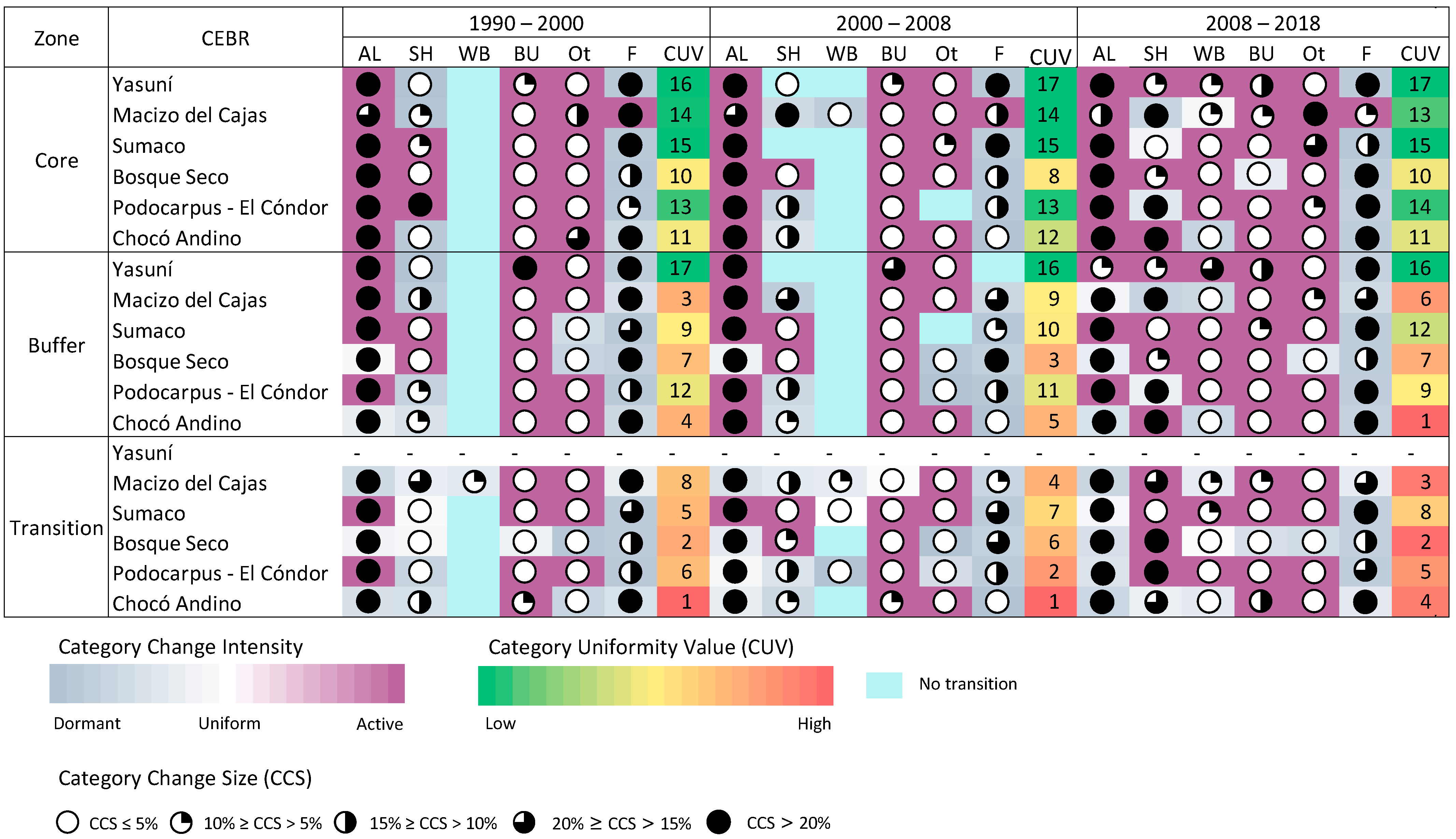
3.2. Category Intensity Analysis–CIA

The CUV rank in Figure 4 shows higher values, mainly in the buffer and transition zones in all CEBRs along the three time intervals. Chocó Andino ranks first in these zones from 1990 to 2018, followed by the transition zones of Bosque Seco in the first and third time intervals and the Podocarpus–El Cóndor’s transition zone in the second time interval. Macizo del Cajas ranks third from 1990 to 2000. The core zones of Bosque Seco and Chocó Andino have medium CUV values.
The CUV rank indicates a relative uniformity pattern in the core zones of Yasuní (16,17,17), Macizo del Cajas (13,13,12), Sumaco (15,15,15), Bosque Seco (9,7,9), Podocarpus–El Condor (12,12,13), and Chocó Andino (10,11,10), showing a global constant rank position from 1990 to 2018. This means that the pattern of change in the core zone is constant according to CUV. A similar finding is registered for the Yasuní buffer zone (17,16,16) and the Sumaco transition zone (14,14,14).
The intensity gains of all categories were mainly active during the third time interval rather than during the first and second time intervals in all CEBRs zones. The categories AL, BU, and Ot show an active change in the three time intervals. The SH category has a mostly dormant intensity of change, and the WB category generally has no transitions, with some exceptions in the transition zone in the first and second periods and in the core zone of the second period. The opposite is true for the third period, where the SH and WB categories show an active intensity of change in almost all cases. None of the categories show a uniform intensity in terms of change.
Overall, the AL category was the most active across all time intervals and zones with larger magnitudes of change, and the BU and Ot categories were the most active categories with the smallest magnitudes of change. The F category was mostly dormant, with change sizes greater than 5%, except for the core zone in Macizo del Cajas.

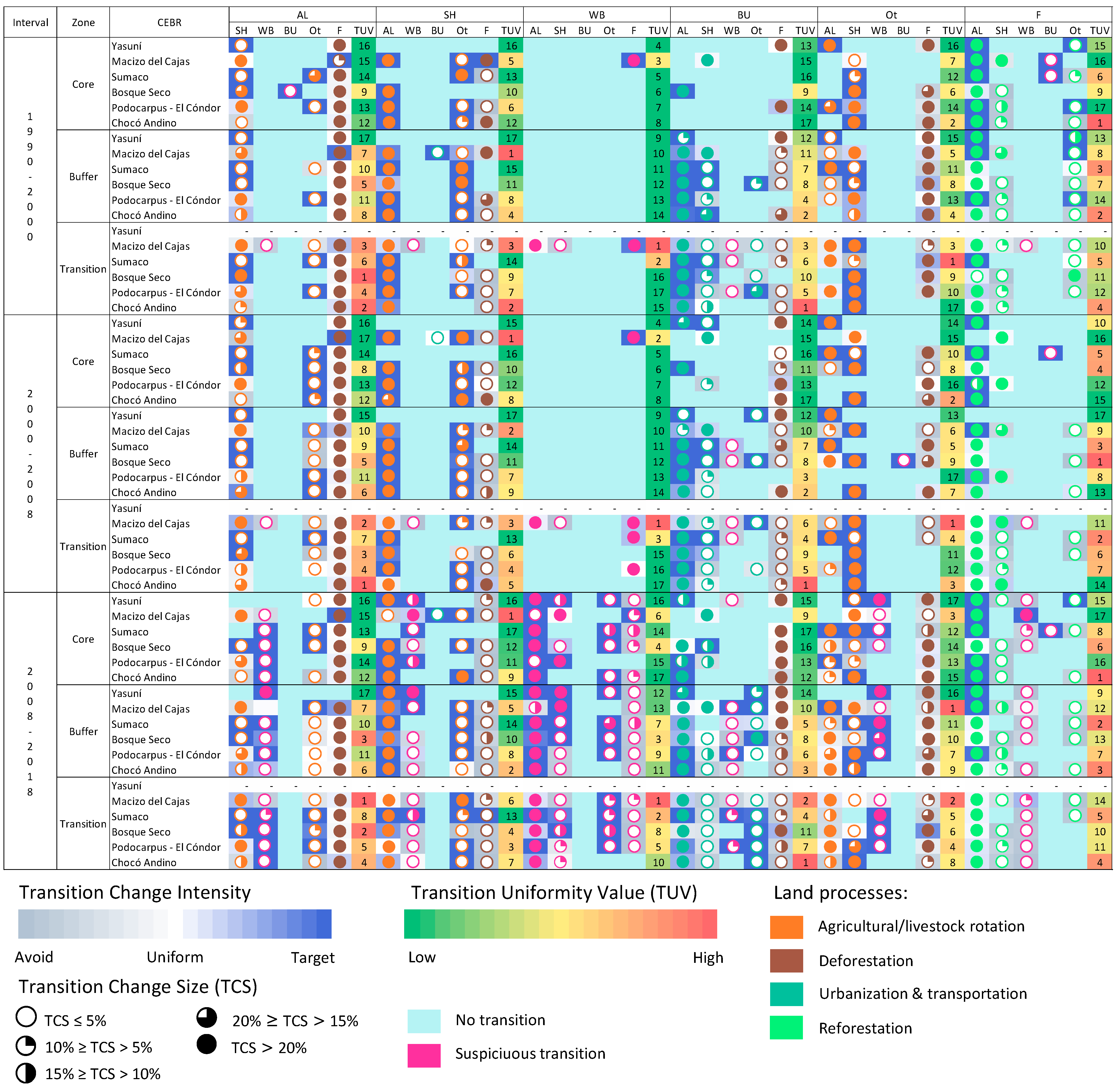
3.3. Transition Intensity Analysis—TIA

Across the three time intervals, in the AL gains, the TUV values are mainly high in the buffer and transition zones in all CEBRs. AL targets SH with different magnitudes of change and Ot mainly with the smallest magnitudes of change. AL mostly avoids F with a magnitude of change greater than 20%, except in the core zone of Macizo del Cajas, where AL targets F with a magnitude of change between 5% and 10% in the first time interval and greater than 20% from 2000 to 2018. AL also targets WB in the last time interval, which was considered a suspicious transition.
In the SH gains, the high TUV values are distributed over all time intervals and CEBR zones, highlighting the core zones of Macizo del Cajas from 2000 to 2018. The intensity and magnitude of change reach high values, especially when SH targets AL. SH avoids F with a tendency to a change in magnitude, mostly less than 5%. SH targets WB in the last time interval, which was again considered a suspicious transition.
WB category gains target other LULC categories in the last time interval, but these were mainly suspicious transitions.
BU’s gains have high TUV in the transition and buffer zones in all time intervals. Chocó Andino ranks first in the transition zone at all time intervals. BU targets AL intensively with a change magnitude greater than 20% in most cases, followed by SH and Ot. BU avoids F, except in the core zones of Podocarpus–El Cóndor from 1990 to 2018. BU targets F in the transition zone of Bosque Seco from 2008 to 2018 with a magnitude of change greater than 20%. Overall, BU avoids WB from 1990 to 2018, but in the last time interval, BU also targets WB in the buffer and transition zones with a change in magnitude of less than 15%. This was considered a suspicious transition.
Ot gains show the high TUV distributed over all time intervals and zones of the CEBRs, even in the core zones, which are protected areas. Ot targets AL and SH with different magnitudes of change. Ot avoids F, except in the buffer zones of Bosque Seco and Chocó Andino and in the transition zones of Sumaco (1990–2000) and Bosque Seco (2008–2018). The Ot category also targets WB from 2008 to 2018, which was considered a suspicious transition.
F gains also show a high TUV distributed across all time intervals and zones of the CEBRs. F targets AL mostly in the core zones and some buffer zones with a magnitude of change greater than 20%. In the transition zones, F avoids AL, except in the Sumaco transition zone from 1990 to 2000.
Crop and livestock rotation occurs when AL shifts to SH or vice versa, SH shifts to Ot or vice versa, and Ot changes to AL. This process is common to all time intervals and zones of the CEBRs and is associated with a common agricultural practice, the fallow period. It does not occur exclusively in the transition and buffer zones, as might be expected, but also in the core zones. The magnitude and intensity of change associated with this process are mostly high and targeted. The crop and livestock rotation is a striking process identified by TIA.
Deforestation occurs when F shifts to AL, SH, BU, or Ot. The intensity of change related to this process is mostly avoided, and the magnitude of the change is relatively high, especially when AL gains from F. There are some exceptions in the AL gains from F, such as the core, buffer, and transition zones of Macizo del Cajas, which show a targeting intensity of change in the three time intervals, with a high magnitude of change. Another exception is in the Ot gains, where the buffer zones of Bosque Seco and Chocó Andino had a targeting intensity of change with the magnitudes of change greater than 20% from 1990 to 2000; this was also observed in the transition zone of Bosque Seco from 2008 to 2018. The deforestation process is also a prominent process in the CEBRs of TIA.
Changes in urbanization and transport infrastructure occur when BU shifts to AL, SH, or Ot. The intensity of change in this process is targeted, especially when BU prefers AL. The magnitude of change associated with urbanization is mostly greater than 5%. This process also occurs in the core zones in all time intervals and zoning of the CEBRs.
The reforestation process occurs when F shifts to AL, SH, or Ot. This process has developed in all zones and time intervals with a magnitude of change greater than 20%.
Some transitions are presented as inconsistent, which is considered a suspicious transition by conventional IA. In Figure 5, these cases have been identified with a pink color for the pie charts, suggesting that this may be part of the classification error of the maps or the effect of climate change because of the dynamics between dry and wet years. The time interval 2008–2018 shows more suspicious transitions, especially in the WB category. This category shows high shifting dynamics between the categories.
Although Figure 5 summarizes 312 bar charts from conventional IA, we have described the most striking transitions. The former order of presenting the results serves as an example to show and discuss all the transitions associated with each land process. In addition, the suspicious transitions can also be traced in terms of intensity and magnitude of change. Specific examples, step-by-step of IIA, CIA, and TIA, are shown in the Supplementary Material.

4. Discussion

4.1. Interpretation of LULC Dynamic Changes in CEBRs

The CEBRs are living scenarios that exhibit (i) persistence and (ii) dynamic shifts in LULC. At the first analysis level, Figure 3 shows the IUV rank, which allows for the easy detection of major interval change intensities to prioritize future actions. A high persistence in the core zones is reflected by lower IUV, suggesting an effective conservation in these areas. Furthermore, the change in magnitude in the Bosque Seco core zone from the 1990s to 2018 is worrying. Other works report similar findings [38,39] but do not compare these across management zones, nor do they use similar management area comparisons with other biosphere reserves.
The year of designation of CEBRs is also a fact that affects the interpretation of LULC changes. This is the case of Chocó Andino, which ranks first in the IUV and has large magnitudes of change from 2000 to 2018 and fast interval change. However, Choco Andino was officially designated as a biosphere reserve in 2018. This biosphere reserve needs attention in the next UNESCO periodic review (2028) to monitor LULC changes. This finding reinforces the idea of reconciling land use conflicts in Choco Andino and supports immediate action, as the situation may be problematic. On the other hand, a slowdown in the intensity of interval change in the coming years could also serve as an example of enhanced land management measures that could be useful for extrapolation to other biosphere reserves. In line with this, the work of Wiegant [40] on the planning of land use realities of the forest and landscape restoration (FLR) objectives of the Bonn Challenge in Choco Andino and Bosque Seco could benefit from evaluating the effectiveness of local measures on land use relevant processes through IIA using IUV as a comparative metric.
In Figure 3, the Bosque Seco transition zone is also a notable site that ranks 3rd in IUV and shows a large size and fast LULC change from 2000 to 2008. This was driven by the expansion of extensive cattle rearing and maize production. The changes occurred in the wet forest remnants between 1000 and 2300 m.a.s.l [41]. This points to the prevention of similar conditions, especially in mountainous landscapes in other biosphere reserves such as Macizo del Cajas-ranked 4th, Podocarpus–El Cóndor-ranked 5th, and Sumaco –ranked 8th.
Composite heat mapping at the IIA level can contribute to LULC modeling during the early stages by displaying overall LULC results in participatory processes. A recent study in northern Ecuador by [42] further discussed the importance of understanding the complexity of LULC change to support LULC modeling and stakeholder engagement in sustainability actions at the local level. In addition, the study highlights the mismatch between national policies and local land use realities. This is an example of how both approaches, IIA composite heat mapping and LULC modeling, could improve land use policy making.
In the second level of analysis (Figure 4), the CUV rank confirms intensive changes among LULC categories in buffer and transition zones. Low overall CUV values indicate persistence in the core zone. In addition, lower values were also found in the Yasuní buffer zone, indicating a low intensive change between categories. This is partly because of the large persistence of the forest category and the smaller changes compared to larger categories, such as agriculture and forests, according to the uniform line of IA. This does not mean that intensive changes in these categories are neglected in LULC change analysis; on the contrary, further analysis with TIA is needed for these areas. One notable shift at the CIA level is between forest and agriculture, and some authors suggest that this shift is not only driven by a deforestation process. For example, in the Sumaco transition zone, part of the shift is due to the expansion of cocoa production using traditional agroforestry systems called chakra. This land process is driven by a change in area of between 0.5 and 4 ha [43]. Despite the impact of this land change in the area, other authors suggest that this process is an essential element for sustainable transition [44] compared to the monoculture agricultural system. On the other hand, the Yasuni buffer zone had a consistent CUV during all of the time intervals because of low anthropogenic intervention. These areas are managed by local communities [45], and low land transformation was confirmed from 1990 to 2018. Inhabitants are committed to the protection of the area since the main livelihoods are dominated by subsistence production and the area is strongly dependent on forests for developing socio-economic activities.
As shown in Figure 4, the CIA increases the level of detail in the analysis by introducing the LULC categories. Most of the changes occurred in the AL, BU, and Ot categories. The CUV in CIA and IUV in IIA for the core zones are similar, corroborating the protection of the core zone. Other approaches [46] also summarize the dynamics of LULC among categories and the issues of current land development patterns in fragile areas in the Three Gorges Reservoir area in China, which is especially associated with reforestation and urban sprawl. This work used the heat map over the transition matrix in percentage and used the concept of the dynamic degree of LULC to quantify the rates of change in different LULC categories within a given time span. However, a limitation in this work concerned the idea of a graphical abridged product being used to analyze LULC dynamics in the time span that includes all categories, as we propose with the composite heat mapping of IA.
LULC changes are the territorial expression of complex interactions that are nontransferable on a spatial or temporal scale between case studies because of the unique properties of territorial development. A challenging objective in monitoring LULC change in biosphere reserves is to provide evidence of financial support to ensure the actual implementation of various policies. Interval (IIA) and category (CIA) assessments will support the implementation of some general policies. However, land processes and ecosystem states will respond to a different set of specific policies, where more detailed information is required to address these policies with greater certainty. In Figure 5, the TIA provides insights into whether a LULC category avoids or targets another category, taking into account the interval and zoning at the same time, allowing comparison across all biosphere reserves. Although this figure reflects the evolution of current land use policies, it does not provide information on the degree of implementation of LULC policies. Nevertheless, the TUV rank between intervals can be compared to assess the progress of policy implementation and its evolution over time.
In Figure 5, one of the most striking and useful results is the color coding of the pie charts to identify land use processes and dynamics. However, in terms of LULC conservation, no transitions are desirable, as shown in light blue cells in the heat map. According to each transition column in Figure 5, WB is the category with the highest number of suspicious transitions, which, in most cases, is due to water logging shifting to vegetated areas, such as humid forests, mangroves, and wetlands during the image classification process. This classification problem has also been reported in other cases in China [47], Mexico [48], and Ecuador [49]. This can be attributed to the misclassification of shadows in images, leading to confusion with other land cover [50]. The WB category in the 2018 LULC map shows potential classification errors because of the suspicious transitions between water bodies and other LULC categories. This can be seen in Figure 5 in the magenta pie charts. Decisions on these transitions need further investigation, especially when WB targets AL and SH with large change magnitudes. In part, this can be attributed to basin irrigation systems and water logging due to heavy rains recorded along the Ecuadorian coast in 2018 [51]. The dynamics over Andean paramo lakes also represent shifts between vegetation and water bodies, which can be attributed to the misclassification of imagery in 2018. River sinuosity also affects inundation areas that shift with vegetation, and meandric river dynamics imply a potential classification error between vegetation and water bodies. Two other classification errors may occur in the coastal environment between water bodies and vegetation, corresponding to the aquaculture of shrimp farms and mangroves. Some authors dealing with these special cases in aquaculture [52] and mangroves [53,54] suggest the careful selection of pure training pixels when defining the classifiers. In the last period of analysis, WB transitions were systematically misclassified, indicating that the classifier or the image source was changed during the implementation of the image classification protocol. It is advisable to users implementing this approach that any interpretation of suspicious transition needs to be deeply assessed, especially for policy making.
In terms of conservation, if F targets AL with large change magnitudes in core areas, this denotes an important result with respect to the effectiveness of reforestation efforts. Similarly, when AL avoids F with high change magnitudes, these are considered prominent cases in almost all CEBR management zones because the change intensity is so low that F is very close to becoming a target of the AL category, implying exacerbated deforestation rates. Another dynamic LULC shift is from SH to AL and vice versa, denoting an active rotation between cropping and livestock rearing. These categories may change intermittently as livestock and cropping are parallel activities of land use in which the rotation may also serve as a soil conservation measure but also as an intensive one. There is no evidence in the literature about the impact of this rotation in Ecuador, but a dynamic between the years indicates an active use of land for cropping and livestock rearing. The effect of these LULC changes in terms of dynamics and intensity warrants further research. Figure 5 is useful for comparison between interval and zoning using TUV. Persistence or low-rank change in TUV indicates continuity in land change or stable management for each land category.
This is the first time that all the information transitions derived from IA are displayed to evaluate the LULC changes, taking into consideration the intensity, magnitude of change, no transitions, suspicious transitions, and land dynamics between different intervals and zoning. The use of heat maps serves to comprehensively display all the information in a condensed form to obtain a ranking to easily track relevant changes compared to changes in other intervals and zones.

4.2. Application of Dimension Reduction and IA in LULC Analysis

Conventional IA and its subsequent extensions have been widely used around the world to study the LULC dynamics of natural and urban landscapes in the context of climate change [55,56], biodiversity [57,58], deforestation [59,60,61,62], urban growth [63,64,65,66,67], environmental risks [68,69], ecosystems [70,71,72], error map quantification [73,74,75], and gender land use preferences [76], among others. These studies share the following common factors in their analyses: a single study area, a set of maps allowing analysis of up to four time intervals, and a set of categories associated with the map layer. Even areas designated as biosphere reserves, where there is zoning, are analyzed in the same way [77]. The results obtained in these studies report the bar charts associated with each level of analysis, which are manageable and understandable when the factors mentioned above are considered. However, if, for example, the zoning of biosphere reserves were included in the analyses, the number of bar graphs would increase, and so would the difficulty of managing and understanding the results.
We propose not only integrating information on the magnitude and intensity of the change in the graph of the third level of analysis, as suggested by [30], but also adding this information to the three levels of analysis. Our approach reveals the magnitudes and intensities of the changes in three heat maps and a classification of the uniform annual rate of change. In addition, the composite heat map of the third level of analysis identifies land processes and suspicious transitions.
This approach allows the inclusion of multiple scales: case studies, zoning, categories, and time intervals. This is useful for decision making in different contexts and management levels. This approach can even be used to report significant LULC changes in the national periodic review report of Biosphere Reserves required by UNESCO every ten years.

4.3. Advantages and Shortcomings

The reporting of LULC change analysis and its results is nowadays an important practice in terms of decision making. The method developed in this work is presented to overcome the problem of summarizing complex sets of IA results. Composite heat mapping is an intuitive tool for displaying multiple results to highlight and easily track changes. Comparisons between zoning areas are also of interest in evaluating evolution or persistence in protected areas. This method offers a straightforward framework to assess multiple aspects simultaneously using graphical summarization when reporting LULC change using the IA method. Four relevant advantages are presented in composite heat maps: (i) the ranking and color coding of uniformity values to quickly identify higher and lower annual changes, (ii) the intensity of change in land transformation through the heat map color ramp, (iii) the magnitude of the change presented in pie charts, and (iv) the color coding included in the pie charts to identify land processes. The intention of the framework proposed does not imply validation of data sets or official maps since the approach is a complementary analysis that highlights suspicious transition detections.
Most policy makers and decision makers are not interested in the processes behind models or methods, but they are interested in concrete results from complex analyses. On the other hand, researchers are constantly confronted with decisions and policy making with a common barrier of balancing between sophisticated methods to overcome complex issues and understanding the knowledge levels of all stakeholders. To overcome this barrier and effectively communicate LULC dynamics, it is necessary to summarize, prioritize, and simplify the results. The framework developed in this work provides the possibility to convey complex LULC dynamics in an inclusive manner, as this framework is a tool that will support dialogue and agreement between stakeholders related to deforestation, forest conservation, urban sprawl, and agricultural expansion.
However, the balance between complex LULC change, decision making, and policy making needs to be handled carefully, as simplification also carries social risks. In order to move beyond risky decisions and to ensure that the results are understood by non-experts, specific assessments need to be made to match the scientific results. This type of assessment, which was not developed in this work, needs to be addressed in the next steps. Advantageously, the approach presented in this work to promote IA in the study of LULC change could be further developed to improve land change science through feedback from participatory stakeholder workshops.
Several works propose different landscape indexes considering territorial processes such as urban sprawl [78,79,80,81,82,83,84,85], cropland expansion [86,87], or deforestation [88,89,90,91,92], in which expansion is usually measured via the buffering of core patches or cumulative maps. The index approach is compatible with composite heat maps with the common aim of characterizing territorial dynamics to quantify multi-temporal changes. Despite the index approach being based on geo-referenced data, it requires technical stakeholders to understand the dynamics of individual patches. Our approach is useful in terms of usability since it summarizes all patches within territorial zoning at three levels of analysis, increasing the detail in the multi-temporal understanding of changes by non-technical stakeholders. Thus, indexing and composite heat maps support various stakeholders to enhance landscape planning issues.
One of the most highlighted challenges is effectively contributing to SDG 15, which among diverse land processes, focuses on reversing land degradation. To halt the land process towards ecosystem degradation, target 15.b, which addresses financial resources for conservation effectiveness, requires comprehensive methods to facilitate financial support assessment using indirect methods as geospatial alternatives. This target is associated with forest management, which is central to most biosphere reserves. The changes in dynamics at three levels of analysis could benefit our understanding of the effectiveness of conservation measures to evaluate the degree of conservation status in temporal and spatial scales through the rankings of IUV, CUV, and TUV. Comparing all core areas of biosphere reserves at intervals, categories, and transitions allows us to confirm that land degradation processes in these areas are scarce, and management could be positively evaluated in the achievement of target 15.1 from a mapping analysis perspective. However, the social science analysis conducted by Krauss in 2022 [93] suggests that despite the SDGs being indivisible, some aspects, such as social and economic matters, are dealt with by other SDGs, and there is no need to address them in SDG 15: Life on Land. Thus, the composite heat mapping of IA is presented as being a valuable tool contributing to SDG 15, but the effect on social and economic interlinkages needs to be cautiously addressed since contextual data are required to be adequately treated in relation to other SDGs.
The Ecuadorian biosphere reserves were used in this work to generate composite heat maps of IA, but this approach is suitable for any case study in which the analysis includes several time intervals, zoning, and multiple categories. In the assessment of ecosystem change, it is recommended to establish common border rules to avoid ecosystem delimitation discrepancies. Image classification with a high accuracy of approximately 70% [94] is advisable when analyzing changes in sensitive ecosystems or highly detailed changes. Biosphere reserve maps derived from supervised classification at 30 m resolution are enough to perform the three levels of analysis, as most areas of the vegetation structural classes occurred at scales ≥ 30 m [95].
The comprehensive framework can support different fields of study related to LULC change to ensure a good understanding of land use changes at different user levels. In future research, various calculations may also be possible, such as composite heat maps to retrieve LULC indices, land process dynamics, and sensitivity analysis of suspicious transitions.

5. Conclusions

An important aspect of LULC change analysis is the effectiveness of the representation and interpretation of results in dynamic areas such as biosphere reserves. The location of specific land processes is also a prime concern for monitoring actions in the short term. Factors relating to time intervals, zoning, and administrative boundaries are needed to propose and design integrated remedial actions. However, the inclusion of all these factors increases the complexity of representing, understanding, and effectively communicating LULC dynamics to decision makers and stakeholders. The implementation of both aggregated and straightforward alternatives is needed to configure effective decisions once this complex LULC change analysis, such as the IA, has been carried out. The framework developed in this work is presented as an alternative to improve the understanding of complex territorial processes, specifically intended to analyze contrasting objectives or cases as the persistence and the dynamic shifts in a comprehensive manner.
The following aspects note the advantages of using composite heat maps for IA:
  • Our work offers an alternative framework for IA to visually identify and rank LULC dynamics in three composite heat maps, one for each level of analysis: interval, category, and transition.
  • The composite heat maps were created based on factors that are commonly considered in the LULC change analysis for decision making. These are multiple areas of interest, zoning, more than three map layer categories, and different time intervals.
  • Each composite heat map integrates information derived from the IA, such as the uniform annual rate classification, the magnitude, and intensity of the change, and at the final level of analysis, it is possible to identify land use dynamics and suspicious transitions of maps through color coding.
  • The simultaneous evaluation of the magnitude and intensity of the change allows an integrated assessment of LULC change.
  • The ranking of uniformity values and color coding is used to identify and prioritize uniform intensity changes at each level of analysis.
  • The composite heat maps provide evidence of the conservation effectiveness of core zones in all CEBRs. In addition, it warns of LULC changes in buffer and transition zones.

Supplementary Materials

The following supporting information can be downloaded at: https://www.mdpi.com/article/10.3390/su16041566/s1, showing a step-by-step example of the calculations and transformation of bar charts to the composite heat map.

Author Contributions

Conceptualization, A.U.-C., D.R.-T., and J.d.l.R.; methodology, A.U.-C., A.G., D.R.-T., and J.d.l.R.; validation, and formal analysis, A.U.-C., D.R.-T., and A.G.; writing—original draft preparation, writing—review and editing, A.U.-C., D.R.-T., A.G., and J.d.l.R.; visualization, A.U.-C.; funding acquisition, A.U.-C. and J.d.l.R. All authors have read and agreed to the published version of the manuscript.

Funding

This research was funded by the Program of the Universidad de Zaragoza–Santander Universidades for supporting doctoral studies of Ibero–Americans.

Institutional Review Board Statement

Not applicable.

Informed Consent Statement

Not applicable.

Data Availability Statement

This manuscript uses data that derived from the following http://ide.ambiente.gob.ec:8080/mapainteractivo/, accessed on 15 July 2023.

Acknowledgments

The first author acknowledges support from Universidad del Azuay through the project “Land use and land cover dynamics in the biosphere reserves of continental Ecuador” under grant number 2023-0090. The authors acknowledge support from the European Union NextGenerationEU and RD 289/2021 and the support of Project No. PGC2018-093854-B-I00 of the Ministerio de Ciencia, Innovación y Universidades of Spain.

Conflicts of Interest

The authors declare no conflicts of interest.

References

  1. Rimal, B.; Sharma, R.; Kunwar, R.; Keshtkar, H.; Stork, N.E.; Rijal, S.; Rahman, S.A.; Baral, H. Effects of land use and land cover change on ecosystem services in the Koshi River Basin, Eastern Nepal. Ecosyst. Serv. 2019, 38, 100963. [Google Scholar] [CrossRef]
  2. Santos, M.J.; Smith, A.B.; Dekker, S.C.; Eppinga, M.B.; Leitão, P.J.; Moreno-Mateos, D.; Morueta-Holme, N.; Ruggeri, M. The role of land use and land cover change in climate change vulnerability assessments of biodiversity: A systematic review. Landsc. Ecol. 2021, 36, 3367–3382. [Google Scholar] [CrossRef]
  3. Fu, Y.; Lu, X.; Zhao, Y.; Zeng, X.; Xia, L. Assessment Impacts of Weather and Land Use/Land Cover (LULC) Change on Urban Vegetation Net Primary Productivity (NPP): A Case Study in Guangzhou, China. Remote Sens. 2013, 5, 4125–4144. [Google Scholar] [CrossRef]
  4. Desta, G.; Tamene, L.; Abera, W.; Amede, T.; Whitbread, A. Effects of land management practices and land cover types on soil loss and crop productivity in Ethiopia: A review. Int. Soil Water Conserv. Res. 2021, 9, 544–554. [Google Scholar] [CrossRef]
  5. Sparrow, B.D.; Edwards, W.; Munroe, S.E.M.; Wardle, G.M.; Guerin, G.R.; Bastin, J.F.; Morris, B.; Christensen, R.; Phinn, S.; Lowe, A.J. Effective ecosystem monitoring requires a multi-scaled approach. Biol. Rev. 2020, 95, 1706–1719. [Google Scholar] [CrossRef]
  6. Allen, C.; Metternicht, G.; Wiedmann, T. Prioritising SDG targets: Assessing baselines, gaps and interlinkages. Sustain. Sci. 2019, 14, 421–438. [Google Scholar] [CrossRef]
  7. Singh, A. Digital change detection techniques using remotely-sensed data. Int. J. Remote Sens. 1989, 10, 989–1003. [Google Scholar] [CrossRef]
  8. Lu, D.; Mausel, P.; Brondízio, E.; Moran, E. Change detection techniques. Int. J. Remote Sens. 2004, 25, 2365–2401. [Google Scholar] [CrossRef]
  9. Brown, D.G.; Walker, R.; Manson, S.; Seto, K. Modeling Land Use and Land Cover Change. In Land Change Science: Observing, Monitoring and Understanding Trajectories of Change on the Earth’s Surface; Gutman, G., Janetos, A.C., Justice, C.O., Moran, E.F., Mustard, J.F., Rindfuss, R.R., Skole, D., Turner, B.L., Cochrane, M.A., Eds.; Springer: Dordrecht, The Netherlands, 2004; pp. 395–409. ISBN 978-1-4020-2562-4. [Google Scholar]
  10. Díaz, S.; Quétier, F.; Cáceres, D.M.; Trainor, S.F.; Pérez-Harguindeguy, N.; Bret-Harte, M.S.; Finegan, B.; Peña-Claros, M.; Poorter, L. Linking functional diversity and social actor strategies in a framework for interdisciplinary analysis of nature’s benefits to society. Proc. Natl. Acad. Sci. USA 2011, 108, 895–902. [Google Scholar] [CrossRef] [PubMed]
  11. Urgilez-Clavijo, A.; Rivas-Tabares, D.A.; Martín-Sotoca, J.J.; Tarquis Alfonso, A.M. Local Fractal Connections to Characterize the Spatial Processes of Deforestation in the Ecuadorian Amazon. Entropy 2021, 23, 748. [Google Scholar] [CrossRef]
  12. Urgilez-Clavijo, A.; de la Riva, J.; Rivas-Tabares, D.A.; Tarquis, A.M. Linking deforestation patterns to soil types: A multifractal approach. Eur. J. Soil Sci. 2021, 72, 635–655. [Google Scholar] [CrossRef]
  13. Verburg, P.H.; Alexander, P.; Evans, T.; Magliocca, N.R.; Malek, Z.; Rounsevell, M.D.; van Vliet, J. Beyond land cover change: Towards a new generation of land use models. Curr. Opin. Environ. Sustain. 2019, 38, 77–85. [Google Scholar] [CrossRef]
  14. Aldwaik, S.Z.; Pontius, R.G. Intensity analysis to unify measurements of size and stationarity of land changes by interval, category, and transition. Landsc. Urban Plan. 2012, 106, 103–114. [Google Scholar] [CrossRef]
  15. Sohl, T.L.; Claggett, P.R. Clarity versus complexity: Land-use modeling as a practical tool for decision-makers. J. Environ. Manag. 2013, 129, 235–243. [Google Scholar] [CrossRef]
  16. Watson, J.E.M.; Dudley, N.; Segan, D.B.; Hockings, M. The performance and potential of protected areas. Nature 2014, 515, 67–73. [Google Scholar] [CrossRef]
  17. Aryal, J.; Sitaula, C.; Frery, A.C. Land use and land cover (LULC) performance modeling using machine learning algorithms: A case study of the city of Melbourne, Australia. Sci. Rep. 2023, 13, 13510. [Google Scholar] [CrossRef]
  18. Quan, B.; Pontius Jr, R.G.; Song, H. Intensity Analysis to communicate land change during three time intervals in two regions of Quanzhou City, China. GIScience Remote Sens. 2020, 57, 21–36. [Google Scholar] [CrossRef]
  19. Haque, M.I.; Basak, R. Land cover change detection using GIS and remote sensing techniques: A spatio-temporal study on Tanguar Haor, Sunamganj, Bangladesh. Egypt. J. Remote Sens. Space Sci. 2017, 20, 251–263. [Google Scholar] [CrossRef]
  20. Talukdar, S.; Singha, P.; Shahfahad; Mahato, S.; Praveen, B.; Rahman, A. Dynamics of ecosystem services (ESs) in response to land use land cover (LU/LC) changes in the lower Gangetic plain of India. Ecol. Indic. 2020, 112, 106121. [Google Scholar] [CrossRef]
  21. Souza, J.M.; Morgado, P.; Costa, E.M.; Vianna, L.F. Modeling of Land Use and Land Cover (LULC) Change Based on Artificial Neural Networks for the Chapecó River Ecological Corridor, Santa Catarina/Brazil. Sustainability 2022, 14, 4038. [Google Scholar]
  22. Zhou, Z.; Quan, B.; Deng, Z. Effects of Land Use Changes on Ecosystem Service Value in Xiangjiang River Basin, China. Sustainability 2023, 15, 2492. [Google Scholar] [CrossRef]
  23. Deng, Z.; Quan, B. Intensity Characteristics and Multi-Scenario Projection of Land Use and Land Cover Change in Hengyang, China. Int. J. Environ. Res. Public Health 2022, 19, 8491. [Google Scholar] [CrossRef] [PubMed]
  24. Lotfollahi, M.; Naghipourfar, M.; Luecken, M.D.; Khajavi, M.; Büttner, M.; Wagenstetter, M.; Avsec, Ž.; Gayoso, A.; Yosef, N.; Interlandi, M.; et al. Mapping single-cell data to reference atlases by transfer learning. Nat. Biotechnol. 2022, 40, 121–130. [Google Scholar] [CrossRef] [PubMed]
  25. Haarman, B.C.B.; Riemersma-Van der Lek, R.F.; Nolen, W.A.; Mendes, R.; Drexhage, H.A.; Burger, H. Feature-expression heat maps—A new visual method to explore complex associations between two variable sets. J. Biomed. Inform. 2015, 53, 156–161. [Google Scholar] [CrossRef] [PubMed]
  26. Cuellar, Y.; Perez, L. Multitemporal modeling and simulation of the complex dynamics in urban wetlands: The case of Bogota, Colombia. Sci. Rep. 2023, 13, 9374. [Google Scholar] [CrossRef]
  27. Gaur, S.; Singh, R. A Comprehensive Review on Land Use/Land Cover (LULC) Change Modeling for Urban Development: Current Status and Future Prospects. Sustainability 2023, 15, 903. [Google Scholar] [CrossRef]
  28. Du, X.; Zhao, X.; Liang, S.; Zhao, J.; Xu, P.; Wu, D. Quantitatively Assessing and Attributing Land Use and Land Cover Changes on China’s Loess Plateau. Remote Sens. 2020, 12, 353. [Google Scholar] [CrossRef]
  29. Zuo, Y.; Cheng, J.; Fu, M. Analysis of Land Use Change and the Role of Policy Dimensions in Ecologically Complex Areas: A Case Study in Chongqing. Land 2022, 11, 627. [Google Scholar] [CrossRef]
  30. Xie, Z.; Pontius, R.G.; Huang, J.; Nitivattananon, V. Enhanced intensity analysis to quantify categorical change and to identify suspicious land transitions: A case study of Nanchang, China. Remote Sens. 2020, 12, 3323. [Google Scholar] [CrossRef]
  31. Ministerio del Ambiente Agua y Transición Ecológica del Ecuador (MAATE). Mapa de Cobertura y Uso de la Tierra del Ecuador Continental año 1990. Available online: http://ide.ambiente.gob.ec:8080/mapainteractivo/ (accessed on 15 July 2023).
  32. Ministerio del Ambiente Agua y Transición Ecológica del Ecuador (MAATE). Mapa de Cobertura y Uso de la Tierra del Ecuador Continental año 2000. Available online: http://ide.ambiente.gob.ec:8080/mapainteractivo/ (accessed on 15 July 2023).
  33. Ministerio del Ambiente Agua y Transición Ecológica del Ecuador (MAATE). Mapa de Cobertura y Uso de la Tierra del Ecuador Continental año 2008. Available online: http://ide.ambiente.gob.ec:8080/mapainteractivo/ (accessed on 15 July 2023).
  34. Ministerio del Ambiente Agua y Transición Ecológica del Ecuador (MAATE). Mapa de Cobertura y Uso de la Tierra del Ecuador Continental año 2018. Available online: http://ide.ambiente.gob.ec:8080/mapainteractivo/ (accessed on 15 July 2023).
  35. Ministerio del Ambiente del Ecuador (MAE). Análisis de la deforestación en el Ecuador Continental 1990–2014; Ministerio del Ambiente de Ecuador: Quito, Ecuador, 2016; pp. 1–43. Available online: http://certificacionpuntoverde.ambiente.gob.ec/libraries/EAlfresco.php/?doc=5708eb09-80c7-4c92-aca0-21dfa0ee711b (accessed on 9 August 2023).
  36. Ministerio del Ambiente del Ecuador (MAE); Ministerio de Agricultura Ganadería Acuacultura y Pesca (MAGAP). Protocolo Metodológico para la Elaboración del Mapa de Cobertura y Uso de la Tierra del Ecuador Continental 2013–2014, Escala 1:100,000. Available online: https://studylib.es/doc/5444265/protocolo-metodológico-para-la-elaboración-del-mapa-de-co (accessed on 18 July 2023).
  37. Ministerio del Ambiente del Ecuador (MAE). Reservas de Biosfera del Ecuador: Lugares Excepcionales; PROSAR: Quito, Ecuador, 2010; pp. 1–149. Available online: https://es.scribd.com/doc/90891486/Reserva-Biosfera-Del-Ecuador (accessed on 11 May 2023).
  38. Ochoa, M.W.S.; Paul, C.; Castro, L.M.; Valle, L.; Knoke, T. Banning goats could exacerbate deforestation of the Ecuadorian dry forest–How the effectiveness of conservation payments is influenced by productive use options. Erdkunde 2016, 70, 49–67. [Google Scholar] [CrossRef]
  39. Rivas, C.A.; Guerrero-Casado, J.; Navarro-Cerillo, R.M. Deforestation and fragmentation trends of seasonal dry tropical forest in Ecuador: Impact on conservation. For. Ecosyst. 2021, 8, 46. [Google Scholar] [CrossRef]
  40. Wiegant, D.; Peralvo, M.; van Oel, P.; Dewulf, A. Five scale challenges in Ecuadorian forest and landscape restoration governance. Land Use Policy 2020, 96, 104686. [Google Scholar] [CrossRef]
  41. Mancomunidad de Municipalidades del Sur Occidente de la Provincia de Loja Mancomunidad Bosque Seco. Available online: https://www.mancomunidadbosqueseco.gob.ec/diagnostico-del-territorio-mancomunado/ (accessed on 13 February 2023).
  42. Lippe, M.; Rummel, L.; Günter, S. Simulating land use and land cover change under contrasting levels of policy enforcement and its spatially-explicit impact on tropical forest landscapes in Ecuador. Land Use Policy 2022, 119, 106207. [Google Scholar] [CrossRef]
  43. Torres, B.; Maza, O.J.; Aguirre, P.; Hinojosa, L.; Günter, S. The contribution of traditional agroforestry to climate change adaptation in the Ecuadorian Amazon: The chakra system. In Handbook of Climate Change Adaptation; Leal Filho, W., Ed.; Springer: Berlin/Heidelberg, Germany, 2015; pp. 1973–1994. [Google Scholar]
  44. Coq-Huelva, D.; Higuchi, A.; Alfalla-Luque, R.; Burgos-Morán, R.; Arias-Gutiérrez, R. Co-Evolution and Bio-Social Construction: The Kichwa Agroforestry Systems (Chakras) in the Ecuadorian Amazonia. Sustainability 2017, 9, 1920. [Google Scholar] [CrossRef]
  45. Loaiza, T.; Nehren, U.; Gerold, G. REDD+ and incentives: An analysis of income generation in forest-dependent communities of the Yasuní Biosphere Reserve, Ecuador. Appl. Geogr. 2015, 62, 225–236. [Google Scholar] [CrossRef]
  46. Zhang, S.; Chen, C.; Yang, Y.; Huang, C.; Wang, M.; Tan, W. Coordination of economic development and ecological conservation during spatiotemporal evolution of land use/cover in eco-fragile areas. CATENA 2023, 226, 107097. [Google Scholar] [CrossRef]
  47. Jiang, W.; Ni, Y.; Pang, Z.; Li, X.; Ju, H.; He, G.; Lv, J.; Yang, K.; Fu, J.; Qin, X. An Effective Water Body Extraction Method with New Water Index for Sentinel-2 Imagery. Water 2021, 13, 1647. [Google Scholar] [CrossRef]
  48. Sandoval, S.; Escobar-Flores, J.G.; Sánchez-Ortíz, E. Inventario de cuerpos de agua de la Sierra Madre Occidental (México) usando SIG y percepción remota. Investig. Geográficas 2020, (102). [Google Scholar] [CrossRef]
  49. Ngoc, D.D.; Loisel, H.; Jamet, C.; Vantrepotte, V.; Duforêt-Gaurier, L.; Minh, C.D.; Mangin, A. Coastal and inland water pixels extraction algorithm (WiPE) from spectral shape analysis and HSV transformation applied to Landsat 8 OLI and Sentinel-2 MSI. Remote Sens. Environ. 2019, 223, 208–228. [Google Scholar] [CrossRef]
  50. Maurya, K.; Mahajan, S.; Chaube, N. Remote sensing techniques: Mapping and monitoring of mangrove ecosystem—A review. Complex Intell. Syst. 2021, 7, 2797–2818. [Google Scholar] [CrossRef]
  51. Pinos, J.; Timbe, L. Mountain riverine floods in Ecuador: Issues, challenges, and opportunities. Front. Water 2020, 2, 545880. [Google Scholar] [CrossRef]
  52. Gusmawati, N.; Soulard, B.; Selmaoui-Folcher, N.; Proisy, C.; Mustafa, A.; Le Gendre, R.; Laugier, T.; Lemonnier, H. Surveying shrimp aquaculture pond activity using multitemporal VHSR satellite images—Case study from the Perancak estuary, Bali, Indonesia. Mar. Pollut. Bull. 2018, 131, 49–60. [Google Scholar] [CrossRef]
  53. Hamilton, S.E. Mangroves and Aquaculture: A Five Decade Remote Sensing Analysis of Ecuador’s Estuarine Environments; Springer: Berlin/Heidelberg, Germany, 2019; Volume 33, ISBN 3030222403. [Google Scholar]
  54. Morocho, R.; González, I.; Ferreira, T.O.; Otero, X.L. Mangrove Forests in Ecuador: A Two-Decade Analysis. Forests 2022, 13, 656. [Google Scholar] [CrossRef]
  55. Tong, S.; Lai, Q.; Zhang, J.; Bao, Y.; Lusi, A.; Ma, Q.; Li, X.; Zhang, F. Spatiotemporal drought variability on the Mongolian Plateau from 1980–2014 based on the SPEI-PM, intensity analysis and Hurst exponent. Sci. Total Environ. 2018, 615, 1557–1565. [Google Scholar] [CrossRef]
  56. Abd El-Hamid, H.T.; Caiyong, W.; Hafiz, M.A.; Mustafa, E.K. Effects of land use/land cover and climatic change on the ecosystem of North Ningxia, China. Arab. J. Geosci. 2020, 13, 1099. [Google Scholar] [CrossRef]
  57. Clements, G.R.; Lynam, A.J.; Gaveau, D.; Yap, W.L.; Lhota, S.; Goosem, M.; Laurance, S.; Laurance, W.F. Where and how are roads endangering mammals in Southeast Asia’s forests? PLoS ONE 2014, 9, 12. [Google Scholar] [CrossRef]
  58. Jewitt, D.; Goodman, P.S.; Erasmus, B.F.N.; O’Connor, T.G.; Witkowski, E.T.F. Systematic land-cover change in KwaZulu-Natal, South Africa: Implications for biodiversity. S. Afr. J. Sci. 2015, 111, 1–9. [Google Scholar] [CrossRef] [PubMed]
  59. Zaehringer, J.G.; Eckert, S.; Messerli, P. Revealing Regional Deforestation Dynamics in North-Eastern Madagascar—Insights from Multi-Temporal Land Cover Change Analysis. Land 2015, 4, 454–474. [Google Scholar] [CrossRef]
  60. Mansaray, L.R.; Huang, J.; Kamara, A.A. Mapping deforestation and urban expansion in Freetown, Sierra Leone, from pre- to post-war economic recovery. Environ. Monit. Assess. 2016, 188, 470. [Google Scholar] [CrossRef] [PubMed]
  61. De Alban, J.D.T.; Jamaludin, J.; Wong de Wen, D.; Than, M.M.; Webb, E.L. Improved estimates of mangrove cover and change reveal catastrophic deforestation in Myanmar. Environ. Res. Lett. 2020, 15, 34034. [Google Scholar] [CrossRef]
  62. Yesuf, G.; Brown, K.A.; Walford, N. Assessing regional-scale variability in deforestation and forest degradation rates in a tropical biodiversity hotspot. Remote Sens. Ecol. Conserv. 2019, 5, 346–359. [Google Scholar] [CrossRef]
  63. Subasinghe, S.; Estoque, R.C.; Murayama, Y. Spatiotemporal analysis of urban growth using GIS and remote sensing: A case study of the Colombo metropolitan area, Sri Lanka. ISPRS Int. J. Geo-Inf. 2016, 5, 197. [Google Scholar] [CrossRef]
  64. Estoque, R.C.; Murayama, Y. Intensity and spatial pattern of urban land changes in the megacities of Southeast Asia. Land Use Policy 2015, 48, 213–222. [Google Scholar] [CrossRef]
  65. Simwanda, M.; Murayama, Y. Spatiotemporal patterns of urban land use change in the rapidly growing city of Lusaka, Zambia: Implications for sustainable urban development. Sustain. Cities Soc. 2018, 39, 262–274. [Google Scholar] [CrossRef]
  66. Sang, X.; Guo, Q.; Wu, X.; Fu, Y.; Xie, T.; He, C.; Zang, J. Intensity and Stationarity Analysis of Land Use Change Based on CART Algorithm. Sci. Rep. 2019, 9, 12279. [Google Scholar] [CrossRef]
  67. Nyamekye, C.; Kwofie, S.; Ghansah, B.; Agyapong, E.; Boamah, L.A. Assessing urban growth in Ghana using machine learning and intensity analysis: A case study of the New Juaben Municipality. Land Use Policy 2020, 99, 105057. [Google Scholar] [CrossRef]
  68. Wang, H.; Feng, R.; Li, X.; Yang, Y.; Pan, Y. Land Use Change and Its Impact on Ecological Risk in the Huaihe River Eco-Economic Belt. Land 2023, 12, 1247. [Google Scholar] [CrossRef]
  69. Vogel, A.; Seeger, K.; Brill, D.; Brückner, H.; Kraas, F. Identifying Land-Use Related Potential Disaster Risk Drivers in the Ayeyarwady Delta (Myanmar) during the Last 50 Years (1974–2021) Using a Hybrid Ensemble Learning Model. Remote Sens. 2022, 14, 3568. [Google Scholar] [CrossRef]
  70. Bauni, V.; Schivo, F.; Capmourteres, V.; Homberg, M. Ecosystem loss assessment following hydroelectric dam flooding: The case of Yacyretá, Argentina. Remote Sens. Appl. Soc. Environ. 2015, 1, 50–60. [Google Scholar] [CrossRef]
  71. Asadolahi, Z.; Salmanmahiny, A.; Sakieh, Y.; Mirkarimi, S.H.; Baral, H.; Azimi, M. Dynamic trade-off analysis of multiple ecosystem services under land use change scenarios: Towards putting ecosystem services into planning in Iran. Ecol. Complex. 2018, 36, 250–260. [Google Scholar] [CrossRef]
  72. Tang, J.; Li, Y.; Cui, S.; Xu, L.; Ding, S.; Nie, W. Linking land-use change, landscape patterns, and ecosystem services in a coastal watershed of southeastern China. Glob. Ecol. Conserv. 2020, 23, e01177. [Google Scholar] [CrossRef]
  73. Enaruvbe, G.O.; Pontius, R.G. Influence of classification errors on Intensity Analysis of land changes in southern Nigeria. Int. J. Remote Sens. 2015, 36, 244–261. [Google Scholar] [CrossRef]
  74. Sun, X.; Li, G.; Wang, J.; Wang, M. Quantifying the land use and land cover changes in the yellow river basin while accounting for data errors based on globeland30 maps. Land 2021, 10, 31. [Google Scholar] [CrossRef]
  75. Tankpa, V.; Wang, L.; Atanga, R.A.; Awotwi, A.; Guo, X. Evidence and impact of map error on land use and land cover dynamics in Ashi River watershed using intensity analysis. PLoS ONE 2020, 15, e0229298. [Google Scholar] [CrossRef] [PubMed]
  76. Villamor, G.B.; Catacutan, D.C.; Truong, V.A.T.; Thi, L.D. Tree-cover transition in Northern Vietnam from a gender-specific land-use preferences perspective. Land Use Policy 2017, 61, 53–62. [Google Scholar] [CrossRef]
  77. Evans, S.W. An assessment of land cover change as a source of information for conservation planning in the Vhembe Biosphere Reserve. Appl. Geogr. 2017, 82, 35–47. [Google Scholar] [CrossRef]
  78. Ismael, H.M. Urban form study: The sprawling city—Review of methods of studying urban sprawl. GeoJournal 2021, 86, 1785–1796. [Google Scholar] [CrossRef]
  79. Kushwaha, K.; Singh, M.M.; Singh, S.K.; Patel, A. Urban growth modeling using earth observation datasets, Cellular Automata-Markov Chain model and urban metrics to measure urban footprints. Remote Sens. Appl. Soc. Environ. 2021, 22, 100479. [Google Scholar] [CrossRef]
  80. Cieślak, I.; Biłozor, A.; Szuniewicz, K. The Use of the CORINE Land Cover (CLC) Database for Analyzing Urban Sprawl. Remote Sens. 2020, 12, 282. [Google Scholar] [CrossRef]
  81. Liu, J.; Jiao, L.; Zhang, B.; Xu, G.; Yang, L.; Dong, T.; Xu, Z.; Zhong, J.; Zhou, Z. New indices to capture the evolution characteristics of urban expansion structure and form. Ecol. Indic. 2021, 122, 107302. [Google Scholar] [CrossRef]
  82. Jiao, L.; Liu, J.; Xu, G.; Dong, T.; Gu, Y.; Zhang, B.; Liu, Y.; Liu, X. Proximity Expansion Index: An improved approach to characterize evolution process of urban expansion. Comput. Environ. Urban Syst. 2018, 70, 102–112. [Google Scholar] [CrossRef]
  83. Liu, J.; Xu, Q.; Yi, J.; Huang, X. Analysis of the heterogeneity of urban expansion landscape patterns and driving factors based on a combined Multi-Order Adjacency Index and Geodetector model. Ecol. Indic. 2022, 136, 108655. [Google Scholar] [CrossRef]
  84. Liu, X.; Li, X.; Chen, Y.; Tan, Z.; Li, S.; Ai, B. A new landscape index for quantifying urban expansion using multi-temporal remotely sensed data. Landsc. Ecol. 2010, 25, 671–682. [Google Scholar] [CrossRef]
  85. Jiao, L.; Mao, L.; Liu, Y. Multi-order Landscape Expansion Index: Characterizing urban expansion dynamics. Landsc. Urban Plan. 2015, 137, 30–39. [Google Scholar] [CrossRef]
  86. Wang, L.; Zhang, S.; Xie, Y.; Liu, Y.; Liu, Y. How Does Different Cropland Expansion Trajectories Affect Cropland Fragmentation? Insights From Three Urban Agglomerations in Yangtze River Economic Belt, China. Front. Ecol. Evol. 2022, 10, 927238. [Google Scholar] [CrossRef]
  87. Chen, H.; Meng, F.; Yu, Z.; Tan, Y. Spatial–temporal characteristics and influencing factors of farmland expansion in different agricultural regions of Heilongjiang Province, China. Land Use Policy 2022, 115, 106007. [Google Scholar] [CrossRef]
  88. Fawcett, D.; Sitch, S.; Ciais, P.; Wigneron, J.P.; Silva-Junior, C.H.L.; Heinrich, V.; Vancutsem, C.; Achard, F.; Bastos, A.; Yang, H.; et al. Declining Amazon biomass due to deforestation and subsequent degradation losses exceeding gains. Glob. Chang. Biol. 2023, 29, 1106–1118. [Google Scholar] [CrossRef]
  89. Bird Reddiar, I.; Osti, M. Quantifying transportation infrastructure pressure on Southeast Asian World Heritage forests. Biol. Conserv. 2022, 270, 109564. [Google Scholar] [CrossRef]
  90. De Matos, T.P.V.; De Matos, V.P.V.; De Mello, K.; Valente, R.A. Protected areas and forest fragmentation: Sustainability index for prioritizing fragments for landscape restoration. Geol. Ecol. Landsc. 2021, 5, 19–31. [Google Scholar] [CrossRef]
  91. Kayet, N.; Pathak, K.; Kumar, S.; Singh, C.P.; Chowdary, V.M.; Chakrabarty, A.; Sinha, N.; Shaik, I.; Ghosh, A. Deforestation susceptibility assessment and prediction in hilltop mining-affected forest region. J. Environ. Manag. 2021, 289, 112504. [Google Scholar] [CrossRef]
  92. Almeida, D.; André, M.; Scariot, E.C.; Fushita, A.T.; dos Santos, J.E.; Bogaert, J. Temporal change of Distance to Nature index for anthropogenic influence monitoring in a protected area and its buffer zone. Ecol. Indic. 2018, 91, 189–194. [Google Scholar] [CrossRef]
  93. Krauss, J.E. Unpacking SDG 15, its targets and indicators: Tracing ideas of conservation. Globalizations 2022, 19, 1179–1194. [Google Scholar] [CrossRef]
  94. Waser, L.T.; Ginzler, C.; Kuechler, M.; Baltsavias, E.; Hurni, L. Semi-automatic classification of tree species in different forest ecosystems by spectral and geometric variables derived from Airborne Digital Sensor (ADS40) and RC30 data. Remote Sens. Environ. 2011, 115, 76–85. [Google Scholar] [CrossRef]
  95. Johansen, K.; Coops, N.C.; Gergel, S.E.; Stange, Y. Application of high spatial resolution satellite imagery for riparian and forest ecosystem classification. Remote Sens. Environ. 2007, 110, 29–44. [Google Scholar] [CrossRef]
Figure 1. Location of the six Continental Ecuador Biosphere Reserves (CEBRs).
Sustainability 16 01566 g001
Figure 2. Methodological workflow. (a) map processing through the zoning of each Continental Ecuador Biosphere Reserve (CEBR) and crosstabulation matrices calculation; (b) graphical representation of conventional Intensity Analysis (IA) at three levels: interval, category, and transition. (c) graphical transformation of conventional IA by d. There is a color-coded correspondence between magnitudes and intensities in blocks (b,c). There is also a correspondence between the first row of the heat map of block (c) and the right side of the bar charts containing d values in block (b). The dashed rectangles in block (c) indicate the change intensity.
Sustainability 16 01566 g002
Figure 3. Intensity and magnitude of the land use and land cover (LULC) changes in the Continental Ecuadorean Biosphere Reserves (CEBRs) by zonation at the interval level. IUV: interval uniformity value.
Sustainability 16 01566 g003
Figure 4. Intensity and magnitude of the land use and land cover (LULC) changes in the Continental Ecuador Biosphere Reserves (CEBRs) by zonation at the category level, showing forest (F), agricultural land (AL), built-up (BU), shrub–herbaceous vegetation (SH), water bodies (WB), and other (Ot).
Sustainability 16 01566 g004
Figure 5. Intensity, magnitude and processes of land use and land cover (LULC) changes in the Continental Ecuador Biosphere Reserves (CEBRs) by zoning at the transition level, showing forest (F), agricultural land (AL), built-up (BU), shrub-herbaceous vegetation (SH), water bodies (WB), and others (Ot).
Sustainability 16 01566 g005
Disclaimer/Publisher’s Note: The statements, opinions and data contained in all publications are solely those of the individual author(s) and contributor(s) and not of MDPI and/or the editor(s). MDPI and/or the editor(s) disclaim responsibility for any injury to people or property resulting from any ideas, methods, instructions or products referred to in the content.

