Research on Spatiotemporal Heterogeneity of the Impact of Earthquakes on Global Copper Ore Supply Based on Geographically Weighted Regression

Abstract

The large and super large copper deposits worldwide are mainly distributed in the Pacific Rim and Gondwana metallogenic domains, and they are highly coupled with the spatial location of seismically active zones. Major copper-producing countries such as Chile are located in areas with high seismic activity. Earthquakes often cause copper mines to shut down, copper prices to soar, and even mining disasters, affecting the stable supply of global copper. In order to study the impact of earthquakes on the global copper ore supply, information on resource endowments, production, and earthquake data from the past 30 years are collected. This article mainly analyzes (1) the spatial correlation between earthquakes and copper mine projects, and the spatial characteristics of earthquakes’ impact on copper mine production, using correlation analysis and geographically weighted regression (GWR); (2) the impact of sudden earthquake events on the export volume and price of copper mines from the perspective of time, using the earthquake index constructed based on the magnitude of the earthquake, the depth of the epicenter, and the distance from the copper mine. The results indicate that the regions with high spatial correlation between copper mine projects and earthquakes are mainly located along the Pacific coast of South and North Americas. Earthquakes can lead to an increase in copper prices, but they will fall significantly in the short term. The impact of earthquakes on export volume generally has a delay period of 1–2 months, resulting in a short-term decrease in export volume. This article quantitatively evaluates the impact of earthquake risk on the supply chain from both spatial and temporal dimensions, providing reference for supply chain risk monitoring, risk impact assessment, and prediction. On the basis of the research results of this article, mineral resource management departments can quantitatively evaluate the spatiotemporal impact of natural risks such as earthquakes on the supply chain, adjust management policies in a timely manner, and improve the level of refined management of supply chain risks.

1. Introduction

Mineral resources are the foundation of modern industrialization and economic development, as well as an important battlefield for major country competition [1,2,3,4]. Copper, as an important industrial raw material, is widely used in fields such as construction, electronics, and transportation. The supply security of mineral resources is crucial, and natural disasters, geopolitical factors, and conflicts can all lead to interruptions in mineral resources [5,6,7,8,9]. Natural disasters are a common cause that affects the stable supply of mineral resources [10]. The large and super large copper deposits worldwide are mainly distributed in the Pacific Rim and the Gondwana metallogenic domains, such as the Phanerozoic orogenic belt, the Precambrian block, and the superimposed Phanerozoic tectonic belt as the tectonic settings [11]. Global strong and large earthquakes often have characteristics of zonal or regional distribution, with their spatial positions basically overlapping with plate boundaries, especially convergent subduction zones. As one of the three main seismic zones, nearly 80% of shallow earthquakes, 90% of medium earthquakes, and almost all deep earthquakes are concentrated in the Pacific Rim seismic zone [12,13,14]. The location of the copper metallogenic belt and the seismic active zone is highly coupled. According to relevant reports and records [15,16] on the impact of earthquakes on copper mine production historically, earthquakes can cause damage to underground facilities, including mines, mining equipment, and ore processing facilities. This may lead to a temporary halt or reduction in copper mine production until the facilities are repaired or rebuilt. In addition, earthquakes may also cause geological disasters, such as landslides and ground subsidence, further affecting the mining and production of copper mines. Thirdly, earthquakes may also have an impact on transportation related to copper mines. Earthquakes may cause damage to infrastructure, such as roads, railways, and ports, thereby hindering the transportation of copper mines. The impact on copper mine production and supply varies depending on the seismic resilience of different facilities [17].

In recent years, the impact of natural disasters has been analyzed, adopting methods such as case analysis and geographic information systems (GIS) [18]. Disaster risk assessments for floods, landslides, and mudslides have been extensively studied [19,20,21,22,23]. In the early stages, some scholars used geographic information system technology and remote sensing methods to draw maps of flood-prone areas and assess flood risk. Amen et al. and Rahmati used remote sensing and geospatial methods to identify flood-prone areas [24]. Souissi Dhekra uses AHP (Analytic Hierarchy Process) to determine the weights of each factor, calculate the flood hazard index, and draw a map of flood-prone areas [25]. On this basis, Xu H proposed a comprehensive method that combines urban flood models, the improved entropy weight method, and the k-means clustering algorithm to draw a flood risk map to evaluate the urban flood risk [26]. In a study on natural disasters’ impact on mineral resources, Wen J et al. used the SVAR model to analyze the relationship between natural and anthropogenic extreme events and oil price risk [27]. Emily Schnebel used the vulnerability model to calculate the expected annual interruption of copper production caused by earthquakes’ EAD (expected annual disruption), quantifying the impact of earthquakes on copper supply in South America [28]. J. Verschuur conducted a ship tracking data analysis to assess the impact of port disruptions caused by natural disasters [29].

It has been proved by spatial econometric methods that there is spatial heterogeneity in socio-economic phenomena [30]. To address the issue of spatial heterogeneity, scholars often use methods such as geographically weighted regression for analysis [31]. The geographically weighted regression analysis technique proposed by Brunsdon (1996) provides an intuitive and practical means of analyzing spatial heterogeneity and multiphase analysis, and it is an important method of local spatial statistical analysis. GWR is usually used in areas such as environment, health, safety, big data analysis, remote sensing, and other fields to explore the differences in different spatial locations [32,33,34]. In recent years, scholars have introduced the GWR model into the study of the spatial heterogeneity of mineral resources, mostly used for energy research. Xu B used local sample data to conduct detailed research on the development of China’s new energy industry using the GWR model, which made up for the shortcomings of previous studies in which the constant coefficient model based on overall sample data could not reveal the spatial heterogeneity of socio-economic phenomena [35,36,37]. Wei L used the GWR model to analyze the impact of energy prices on China’s carbon emissions from a spatial perspective [38].

In summary, earthquakes may cause interruptions or reductions in mineral resource production. Currently, few scholars have quantitatively studied the spatiotemporal impact of earthquakes on global copper supply security. Several scientific issues remain unresolved, such as the scope of the impact of earthquakes on global ore production and supply, as well as the duration and intensity of earthquake interruptions.

The purpose of this article is to analyze the impact of seismic risks on the safety of copper mines’ supply. We use methods such as spatial analysis and instance analysis to analyze the impact of earthquakes on copper mine production, supply, and prices. This article takes the global copper mine project as the research object and analyzes the impact of earthquakes on global copper ore supply from both spatial and temporal dimensions based on earthquake data from the past 30 years. From the spatial perspective, this article uses the method of spatial geographic weighting regression (GWR) to analyze the correlation between copper mines and the location of earthquakes. In previous studies, GWR methods were used to calculate the degree of spatial differentiation among countries from a macroperspective. In order to further explore the spatial correlation among different copper mines, we divide the global surface into a fine-grained spatial unit and use this method for the relevant calculations. On the basis of the results of the GWR, we propose an earthquake index to evaluate the degree of damage caused by earthquakes to copper mines historically, which takes into account the spatial heterogeneity. The spatial range of the impact of earthquakes on copper mine production is estimated using the k-means clustering algorithm to draw an earthquake risk map of copper mines. Unlike previous studies that only focused on the spatial impact of natural disaster risk, the duration and delay time of earthquakes’ impact on the copper supply and market are obtained from a time perspective by analyzing the export volume and futures price changes to the country after the earthquake. The spatiotemporal heterogeneity characteristics of earthquakes’ impact on the copper supply are summarized. This provides a new approach for studying the impact of natural risk factors on mineral resource supply, helping to further carry out global copper supply chain evaluation and safety monitoring.

2. Research Methodology

2.1. Methods

2.1.1. Correlation Analysis

Correlation analysis is used to reflect the degree of interdependence between two elements, that is, the correlation calculation (Equation (1)) between the distribution of copper mines in the grid and the location of earthquakes is:

$$r_{xy}=\frac{\sum \left(x_i-\overline{x}\right)\left(y_i-\overline{y}\right)}{\sqrt{\sum {\left(x_i-\overline{x}\right)}^2\sum {\left(y_i-\overline{y}\right)}^2}}$$

(1)

In Equation (1), $r_{xy}$ is the correlation coefficient between two elements; $x_i$ and $y_i$ are the corresponding element samples ($i=1,2,\dots ,n$); and $\overline{x}$ and $\overline{y}$ are the sample averages of the two elements. $-1\le r_{xy}\le 1$, $r_{xy}>0$ indicates a positive correlation; that is, the two elements are related in the same direction; $r_{xy}<0$ indicates a negative correlation, and the two elements are negatively correlated in opposite directions. The closer the absolute value of $r_{xy}$ is to 1, the closer the relationship between the two elements, and vice versa, the more distant. When $\left|r\right|$ > 0.95, there is a significant correlation; when $\left|r\right|\ge$ 0.8, they are highly correlated; when 0.5 $\le \left|r\right|<$ 0.8, they are moderately correlated; when 0.3 $\le \left|r\right|<$ 0. 5, there is a low degree correlation; and when $\left|r\right|<$ 0.3, the relationship between the two elements is extremely weak, and they are not correlated.

2.1.2. Geographically Weighted Regression Model (GWR)

GWR is a local linear regression model that considers the spatial heterogeneity of variables. It incorporates the position information of the sample points into the regression parameters, and the relationships among variables can vary with the changes in spatial position, which effectively handles spatial nonstationarity. Because of the weak diagnostic performance of GWR models, ordinary least squares regression (OLS) is generally required before a GWR analysis to ensure the accuracy of the model. The regression expressions for GWR and OLS are as follows:

$$y_i={\beta }_0\left(u_i,v_i\right)+{\displaystyle \sum }_{j=1}^k{\beta }_j\left(u_i,v_i\right)x_{ij}+{\epsilon }_i$$

(2)

$$y_i={\beta }_0+{\displaystyle \sum }_{j=1}^k{\beta }_j{x}_{ij}+{\epsilon }_i$$

(3)

In the equations, $x_i$ and $y_i$ refer to the regression independent variable and the dependent variable; ${\beta }_0$ and ${\beta }_0\left(u_i,v_i\right)$ are the global and i-th sample constant terms, respectively; and ${\beta }_j\left(u_i,v_i\right)$ refers to the regression coefficients of the i-th sample and the j-th parameter, reflecting the spatial differentiation of the impact of different parameters on the sample. The positive and negative signs of the coefficients represent the positive and negative correlation properties of the parameters with spatial positions, and the magnitude represents the strength of the correlation; $\left(u_i,v_i\right)$ refers to the coordinates of the i-th sample space; $x_{ij}$ refers to the j-th parameter value of the i-th sample; ${\epsilon }_i$ represents the random error term; and $k$ represents the number of independent variables.

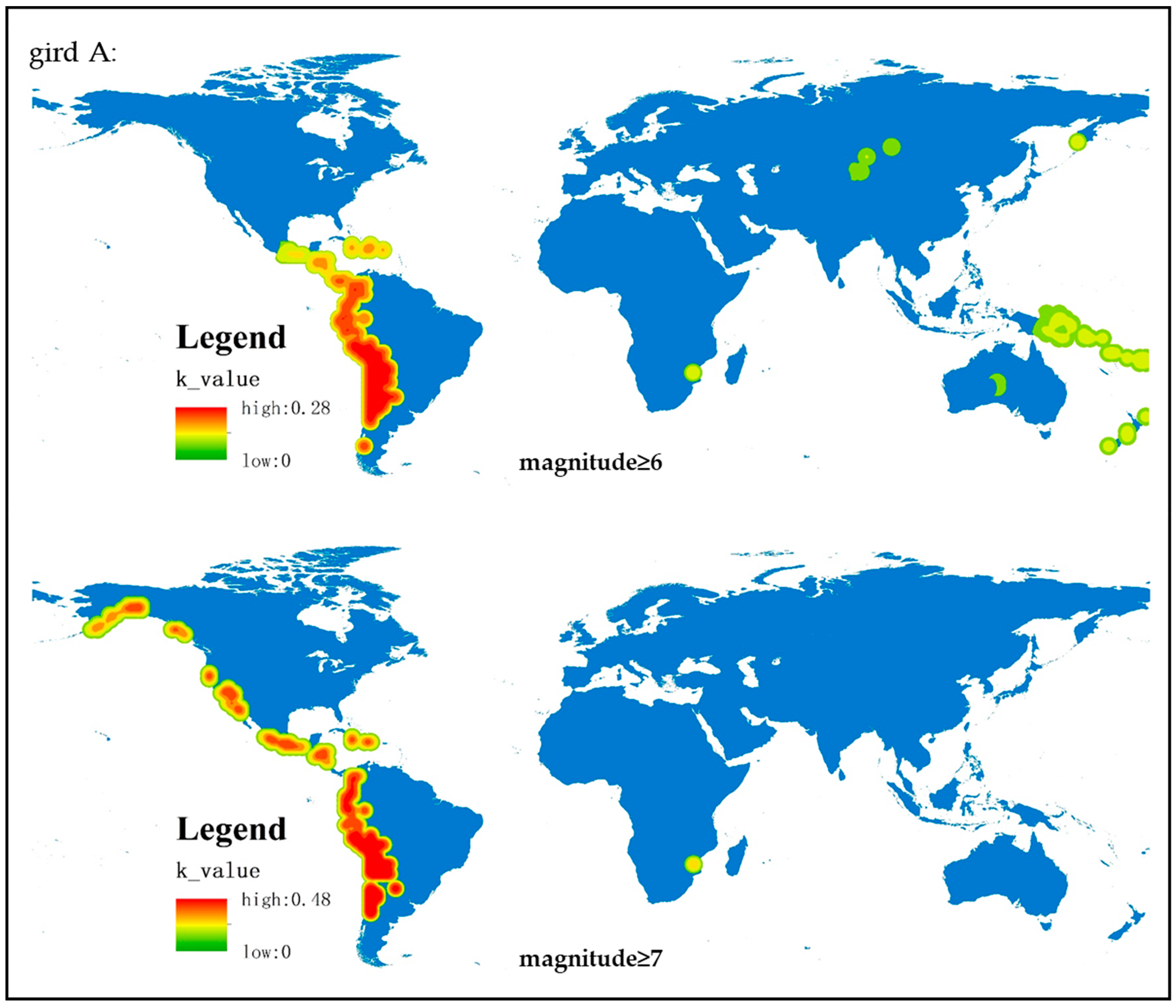
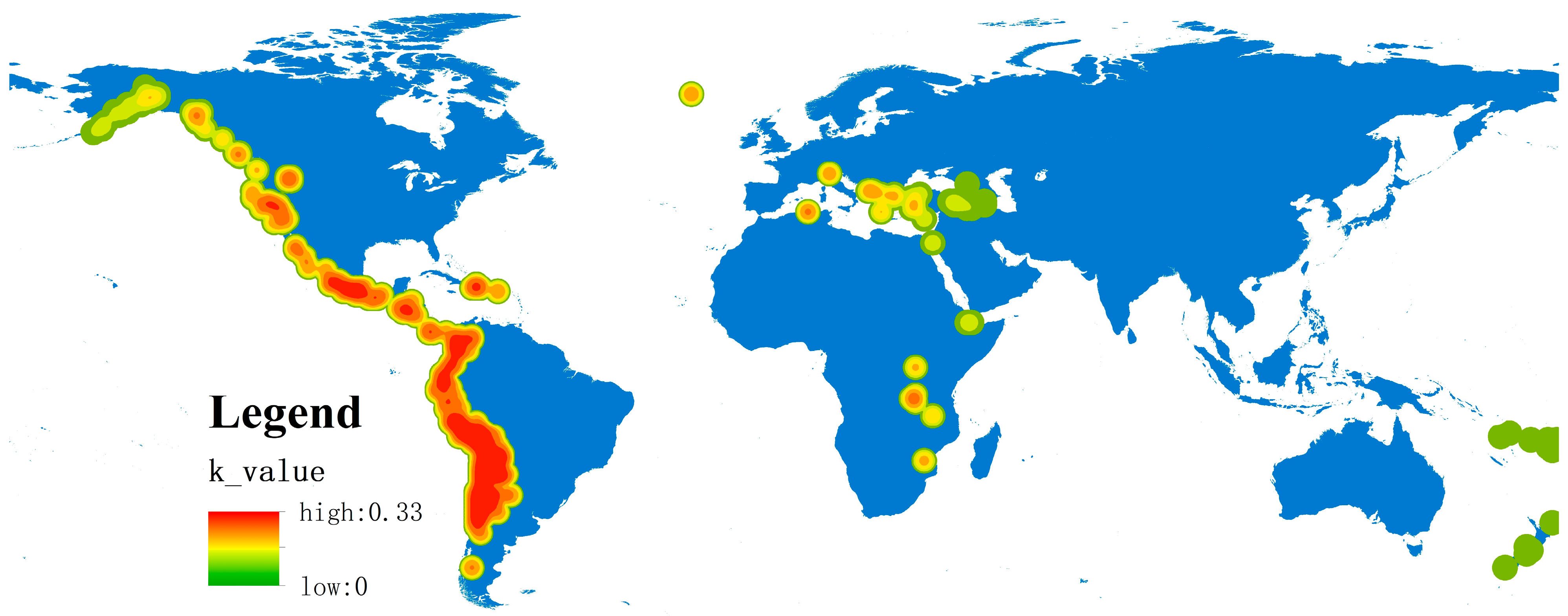
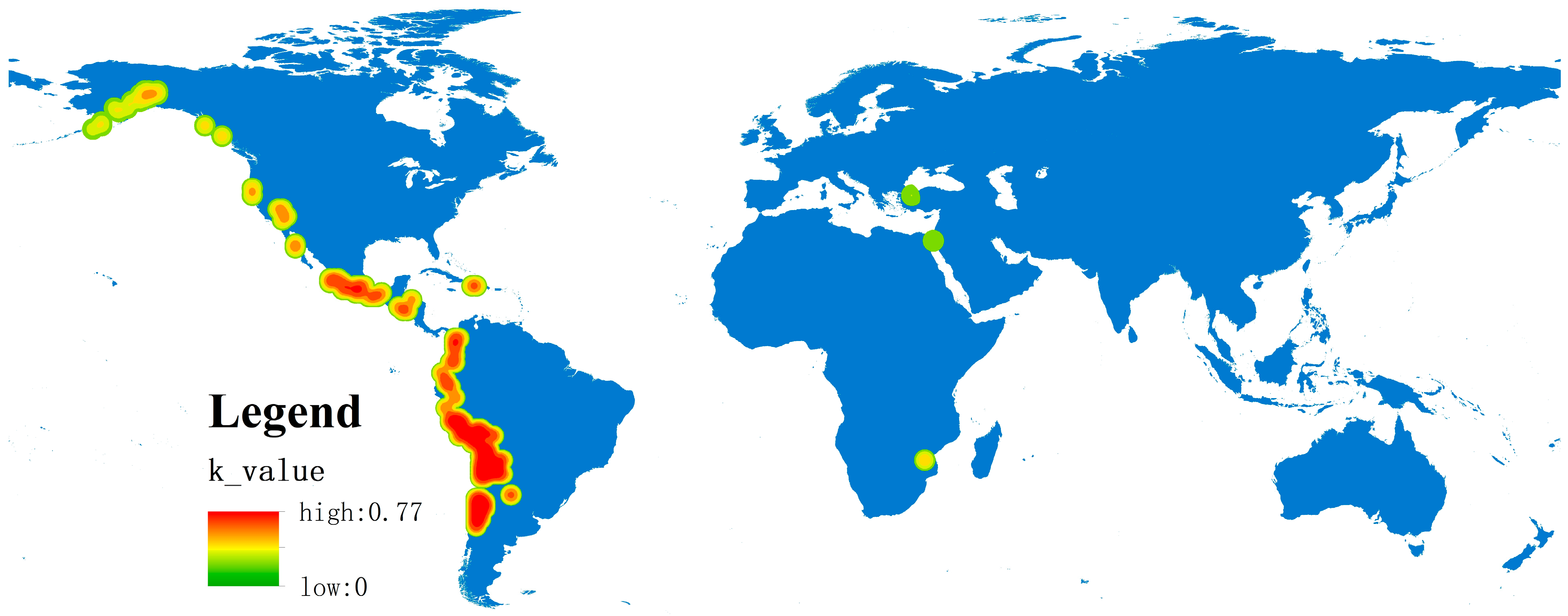
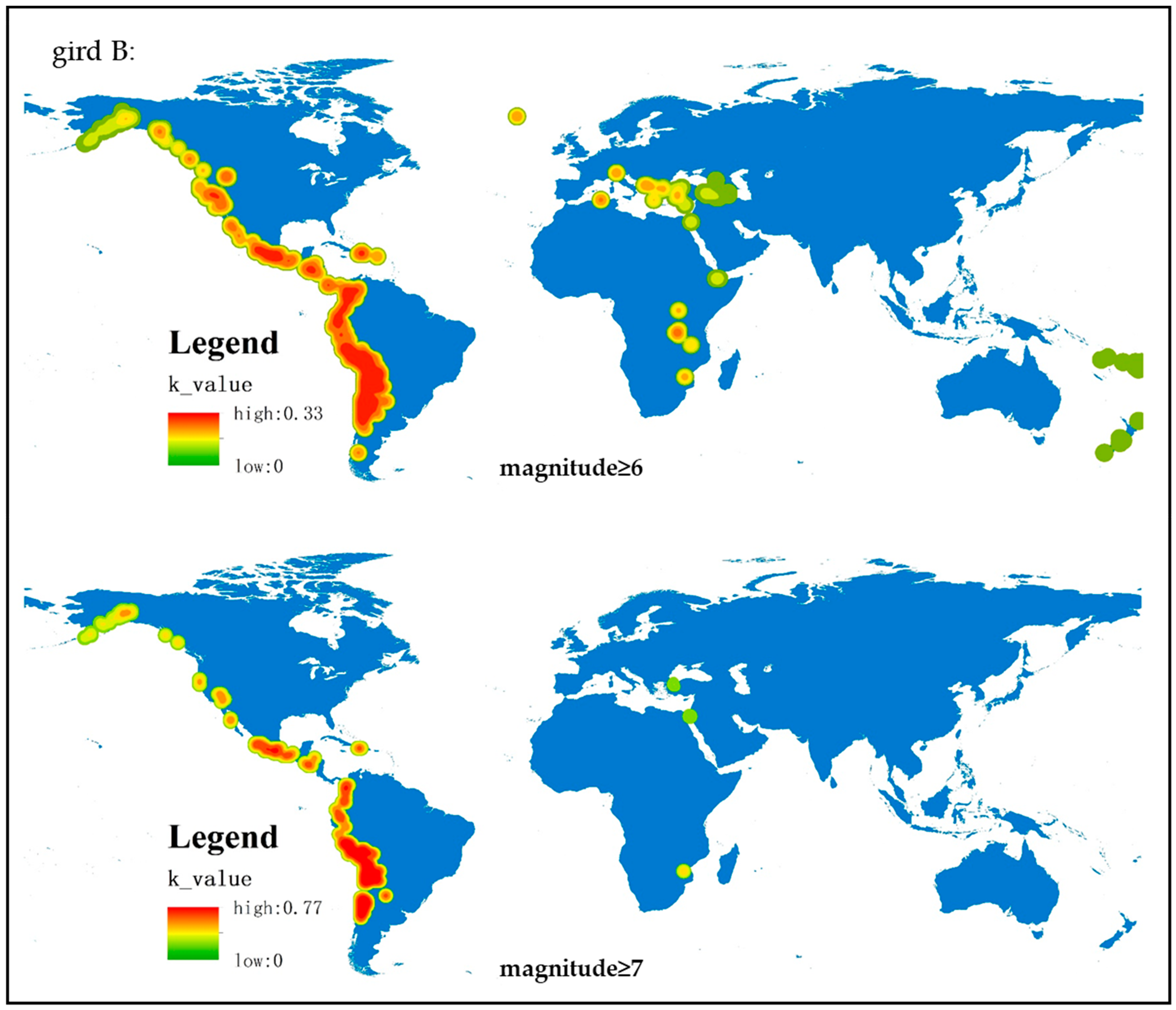
2.1.3. Kernel Density Analysis

Kernel density analysis is used to calculate the density of a feature in its surrounding neighborhood. The surface value is highest at the location of the point, and it gradually decreases as the distance from the point increases. At the location where the distance from the point is equal to the search radius, the surface value is zero. The following Equation (4) defines the method for calculating kernel density:

$$Density=\frac{1}{r^2}{\displaystyle \sum }_{i=1}^n\left[\frac{3}{\pi }\ast po{p}_i{\left(1-{\left(\frac{dis}{r}\right)}^2\right)}^2\right]$$

(4)

In the Equation (4): i is the input point. If they are within the radius distance of position (x, y), only the points in the total are included. $Po{p}_i$ is the population field value of point i, which is an optional parameter. This article uses the GWR correlation coefficient as the population field value. $Dis$ is the distance between point i and position (x, y). Draw a spatial variation map of the regression coefficients of the GWR model based on the results of kernel density analysis.

2.1.4. Earthquake Index

In previous studies, scholars used seismic intensity indicators to evaluate the degree of earthquake damage, or to analyze the probability of a specific seismic intensity forming in an area, in order to assess the seismic hazard of that area [39]. Seismic intensity represents the degree of damage in the epicenter area of an earthquake, and as the distance from the epicenter increases, the degree of earthquake impact decreases. This article considers the spatial heterogeneity of earthquake impact and proposes an earthquake index: on a monthly basis, the earthquake index is weighted based on the magnitude, depth, and distance from the copper mine project of a historical earthquake in a certain area to evaluate the degree of earthquake damage. The magnitude, depth, and location of an earthquake determine its degree of damage. The magnitude of an earthquake indicates its strength, and the larger the magnitude, the more energy an earthquake releases. Generally, earthquakes with a magnitude of six or higher are considered strong earthquakes, which may cause widespread damage and casualties. According to the depth of the earthquake, it is divided into shallow earthquake, medium earthquake, and deep earthquake. The shallower the depth, the greater the destructive power of the earthquake. The regression coefficient of GWR is used to refer to the distance between the earthquake location and the copper mine location. The larger the regression coefficient, the greater the impact of the earthquake on the copper mine. Weighted statistical analysis of the magnitude, depth, and GWR regression coefficients of all earthquakes within the grid to obtain the seismic index at the grid location.

2.2. Data

The copper mine project data used in this article come from the global S&P Capital IQ platform. The monthly export data of copper ore come from UN Comtrade. The seismic catalog data come from the ANSS comprehensive seismic catalog of the United States Geological Survey (USGS), which includes parameters such as source, magnitude, depth, phase pickup, and amplitude. Copper price data come from London Metal Exchange(LME) in Wind Information. This article collects reports on the impact of earthquakes on copper mining areas from historical news reports, and the results are shown in

Table 1. The impact of earthquakes on mining areas in news reports.

Time	Magnitude	Place	Related Reports
12 November 1996	7.3	Peru	Thirteen miners were trapped in the mining area, with water, electricity, and communication affected, roads blocked, and two bridges destroyed.
13 June 2005	7.8	Chile	Cerro Colorado is 10 km away from the epicenter, and road traffic was affected for two weeks after the disaster, causing damage to the factory.
14 November 2007	7.7	Chile North	Many large copper mines are also located in the earthquake zone, and more than ten mines were temporarily shut down due to power outages.
27 February 2010	8.8	Central and Southern Chile	The earthquake triggered a tsunami, with the epicenter still far from the northern region where copper mines are concentrated. However, the earthquake caused power supply disruptions, and four copper mines near the capital Santiago, including Los Bronces, El Soldado, El Tenien, and Andina, were shut down.
3 January 2011	7.2	Central Chile	The depth of the epicenter is 30 km, and the epicenter is about 590 km away from the capital city of Santiago, Chile. Mobile communication and power supply in the earthquake-stricken area have been interrupted.
2 April 2014	8.2	Northern Chilean waters	Occurred along the coast 86 km away from the northern Iquik mining area. The earthquake did not cause any casualties but caused multiple power outages in the northern region, and communication was also affected to some extent.
26 May 2019	7.8	Northern Peru	The depth of the epicenter is 100 km, and the epicenter is far from the main copper mining areas in Peru, with no mining areas affected. The nearby copper mine is Tantahuatay, but there have been no reports of damage.
1 March 2019	7.2	Southern Peru	The depth of the epicenter is 257 km, with a distance of 120 km from the mining area. The southern part of Peru is the main copper-producing area in Peru. Because of the scarcity of personnel near the epicenter, there have been no reports of casualties or property damage caused by the earthquake.
26 December 2004	9.3	West side of Sumatra, Indonesia	Unrecorded.
8 September 2017	8.4	Coastal Mexico	There are no major copper mines in the areas affected by the two earthquakes, so the impact on copper production in Mexico is relatively small, and the impact on its copper concentrate export business to China is relatively small.
19 September 2017	7.1	Morelos State, Central Mexico

.

3. Results

3.1. Spatial Correlation Analysis

From 1992 to 2021, there were more than 4600 earthquakes with a magnitude of M ≥ 6.0 and 450 earthquakes with a magnitude of M ≥ 7.0 worldwide. Figure 1 shows the kernel density map of earthquakes with a magnitude of M ≥ 6.0. Using the magnitude as the population field, over the past thirty years, the global strong earthquake zones have mainly been concentrated in the Pacific Rim and Eurasian seismic zones, mainly occurring in countries or regions such as Chile, Peru, Mexico, Indonesia, and Japan.

Porphyry copper deposits are mainly distributed in the Pacific Rim metallogenic domain, Central Asian metallogenic domain, and Tethyan metallogenic domain, with a focus on the South American Andes metallogenic belt in the Pacific Rim metallogenic domain [40]. Global copper mine projects are mainly distributed in South America, with Chile and Peru being the main copper-producing countries in South America. The Andean metallogenic belt, where Chile and Peru are located, is located on the edge of the NW and near SN trending main faults parallel to the western Pacific deep-sea trough (subduction zone) and is the most important porphyry copper mineralization belt in the world.

Chile and Peru experienced 131 earthquakes with a magnitude of 6 or higher from 1992 to 2021. To understand the potential correlation between seismic activity and the distribution of copper resources, this paper uses correlation analysis to verify the overall spatial correlation. Considering the weight of geographic space, geographic weighted analysis is used to verify the correlation between copper projects and earthquake locations in different regions.

The method described in this article was implemented in ArcGIS. Because earthquakes are point data, they cannot represent the impact range of earthquakes, and spatial analysis methods are used to represent the impact range of earthquakes. On the basis of the damage areas of earthquakes of different levels in the past, a buffer zone is set for earthquakes at the distance shown in

Table 2. Earthquake buffer zone.

Mag.	Earthquake Effect	Buffer (Miles)
6–6.9	Can destroy residential areas within a radius of 100 miles	50
7–7.9	Can cause serious damage to larger areas	100
8–8.9	Can destroy an area for hundreds of miles in a radius	200
9 and above	Destroys an area thousands of miles around	500

. According to the latitude and longitude network, the world is divided into 180 × 360 grids, and the copper mine information and earthquake information falling within each grid are counted. The subsequent spatial correlation analysis was conducted on grid data. On the basis of the global spatial correlation analysis, the Pearson coefficient of the two can be calculated to be 0.586, indicating a high dependence of the project on earthquake distribution and a moderate correlation. There is a spatial coupling relationship between seismic activity and copper mine projects.

According to the OLS diagnostic result (p < 0.01), a regression model with statistical significance and nonsteady state is suitable for geographic weighted regression (GWR) analysis [41]. The GWR model has different regression coefficients in different countries, reflecting differences in the correlation between the location of earthquakes and the distribution of copper mine projects in different regions. The following figure shows the kernel density plot of the GWR model regression coefficients for the locations of earthquakes with a magnitude of 6 or above and the distribution of copper mine projects. Figure 2 (above magnitude 6) shows a high correlation between the two in South America, North America, and southern Africa, whereas Figure 3 (above magnitude 7) shows that the regions with a high correlation are mainly located along the Pacific coast of South America and North America, with regression coefficients higher than magnitude 6. Earthquakes with a magnitude of 7 or higher are more correlated with the distribution of copper mine projects.

The area shown in Figure 3 is a high-risk earthquake area for copper mining projects, which are more susceptible to the impact of earthquakes. According to

Table 3. GWR correlation coefficients of major countries and their impact on mine production.

Country	C_7	Continent	Mines in Earthquake-Affected Areas	Mine Production (Ten Thousand Tons)
Chile	0.66	South America	Escondida, Collahuasi, El Teniente, Radomiro Tomic, Los Pelambres, Los Bronces, Chuquicamata, etc.	470.97
Peru	0.59	South America	Cerro Verde, Toromocho, Antapaccay, Marcona, etc.	114.59
Argentina	0.68	South America	San Jorge	0
Mexico	0.32	North America	Capela, El Aguila, Campo Morado	0.56
Bolivia	0.63	South America	San Vicente	0.05
Colombia	0.47	South America	El Roble	0.68
United States	0.12	North America	-	0
Ecuador	0.51	South America	Mirador	12.5
Indonesia	−0.1	Asia	Grasberg, Wetar	73.03
Philippines	−0.1	Asia	Atlas Toledo, Padcal	4.51
Total				676.9

, there is a positive correlation between the number of copper mine projects and the number of earthquakes in countries such as Chile and Peru. The production of mines in earthquake locations is 5.994 million tons, accounting for 31% of the total copper mine project production in 2022. Nearly one-third of copper ore production may be affected by earthquakes. The distribution of copper mine projects in Indonesia and the Philippines is negatively correlated with the location of earthquakes. The two countries are earthquake prone, with copper mines located on high plateaus and less affected by earthquakes.

According to

Table 4. Resource reserves in earthquake high-risk areas of copper projects.

Development Stage	Projects Number	Resource Reserves (Ore Quantity/Ten Thousand Tons)
Grassroots	61	0
Exploration	106	150
Target Outline	81	30,940
Reserves Development	51	1,981,165
Advanced Exploration	12	60,600
Prefeas/Scoping	12	1,436,647
Feasibility	11	794,016
Feasibility Started	2	4500
Feasibility Complete	4	540,310
Preproduction	3	110
Construction Planned	2	87,080
Operating	71	9,324,633
Satellite	8	0
Expansion	8	6,558,280
Limited Production	3	2204
Closed	9	6030
Total	444	20,826,666.6

, the global copper mine project reserves 600 billion tons, mainly distributed in the Americas. There are a total of 444 copper mine projects in earthquake high-risk areas, with resource reserves accounting for 34% of the global total. In earthquake high-risk areas, the main projects are those in the Grassroots, Exploration, Target Outline, Reserve Development, and Operating stages, accounting for 83% of the total number of projects in earthquake high-risk areas. The proportion of resource reserves varies in different exploration stages, with the Operating stage accounting for 45% of the resource reserves in earthquake high-risk areas and the Expansion stage accounting for 31%.

Through modeling and calculation, there is a certain spatial correlation between earthquakes and copper mine projects, and earthquakes have a significant impact on copper mining production in Chile and Peru. The reserves and production of global copper mine projects are more than 30% affected by earthquakes, and earthquakes cause a higher risk in copper supply.

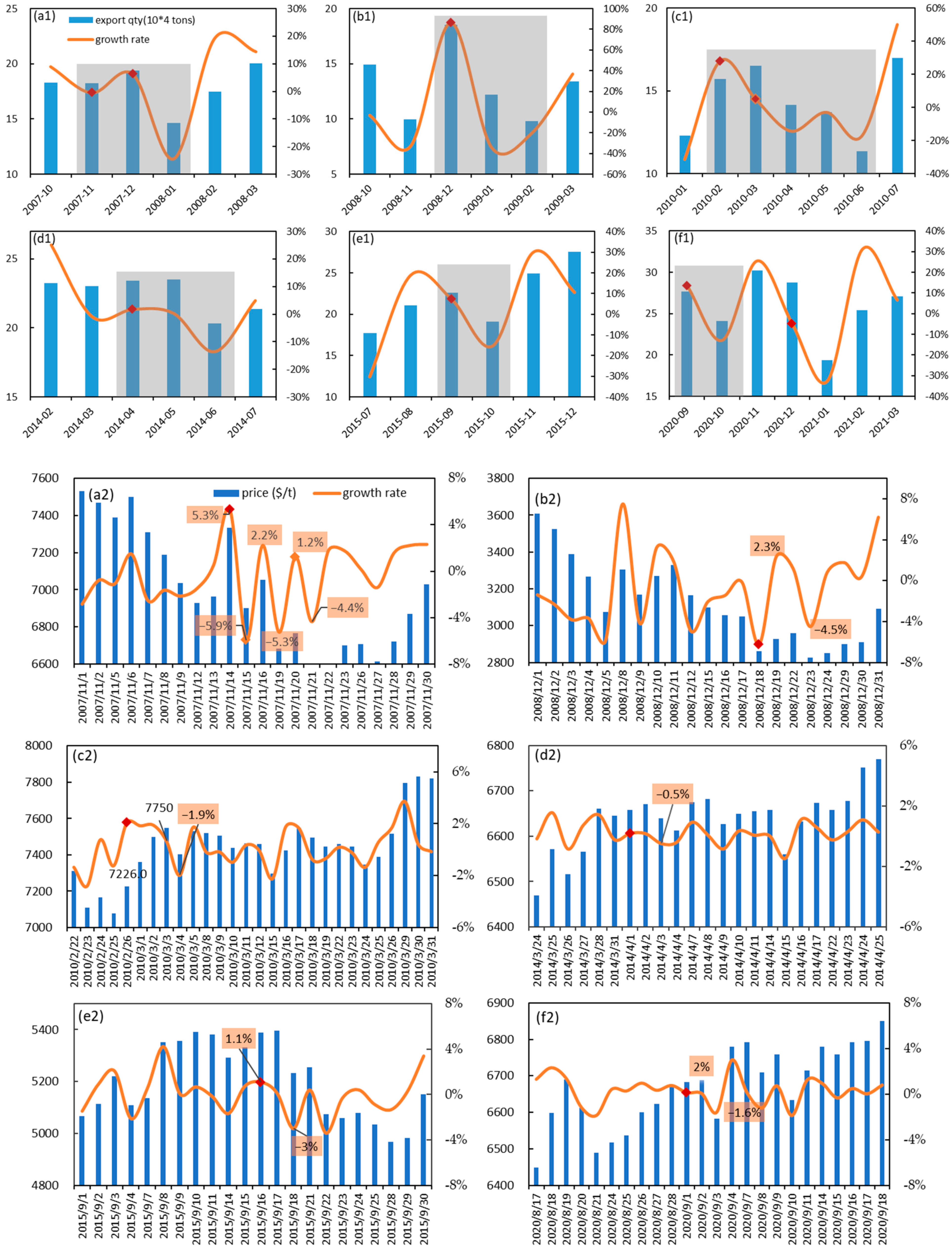
3.2. Time Scale Impact: Chile and Peru

On the basis of the results above, further research is carried out to determine whether copper production and supply are affected by earthquakes. Considering the results of GWR models in major exporting countries and various countries, this article mainly focuses on Chile and Peru, collecting monthly export data and copper ore price data from the two countries over the past 30 years. The earthquake index is determined based on the magnitude of an earthquake, the depth of the epicenter, and the distance from the copper mine. High values for the earthquake index are observed, which refer to the impact of sudden earthquake events on the export volume and price of copper mines, and we explored the relationship between earthquakes and copper mine supply.

Approximately 30% of global copper is produced in Chile, with most copper mines concentrated in the northern regions. Codelco, the Chilean national copper company, is the world’s leading copper producer. Mining giants such as BHP Group Limited and Anglo American plc have invested heavily in Chile and own copper mines in the north. Chile has experienced 54 earthquakes of magnitude 6 or above and 10 earthquakes of magnitude 7 or above over the past 30 years.

By comparing the export data of these time periods, we can observe the impact of earthquake events on the export volume and price of copper mines. In this section, six time periods with higher earthquake indices in Chile were selected, as shown in Figure 4:

(a)

On 14 November 2007, a 7.7-magnitude earthquake occurred in the northern region of Chile, causing two deaths and 100 injuries. Many large copper mines, such as Chuquicamata SX-EW, Spence, Michelle/Lince, and Spence SX-EW, were located in the earthquake zone. Because of the impact of the earthquake, the mines were temporarily shut down and the road to a nearby copper mine in the capital, Santiago, was also blocked. On the same day, copper prices in London surged 5.3% from 6965 USD/ton to 7335 USD/ton and fell 5.9% the next day. Aftershocks occurred on the 15th and 20th, and copper prices showed a pattern of first rising and then falling, with the decline greater than the increase. Two months after the earthquake, Chile’s export volume decreased by 24% compared to the previous month, and it rebounded in February 2008;

(b)

On 18 December 2008, copper prices rose by 2.3% one day after the earthquake and fell by 4.5% four days later. After the earthquake, the export volume decreased continuously for two months and resumed growth in export volume in March. The 2008 financial crisis led to a global economic slowdown and a decrease in copper demand;

(c)

From February to March 2010, Chile experienced 8 earthquakes with a magnitude of 6 or higher. The copper mines were located far from the epicenter, but the earthquakes caused significant damage to infrastructure and had a long-term impact on copper production and transportation. On 27 February, an 8.8-magnitude earthquake occurred, accompanied by aftershocks on the 27th and 28th. The price of London copper continued to rise, with a cumulative increase of over 4%. It reached a high of 7550 USD per ton on March 3rd and fell back on March 4th. One month after the earthquake, the export volume decreased by 14% year-on-year and continued to decline for three months;

(d)

On 1 April 2014, a magnitude 8 earthquake occurred in the northern waters of Chile, with Cerro Colorado and Reina Hija nearby, but the company stated that it did not affect production. The cumulative increase in copper prices over the prior two days was 0.4%, and it quickly fell on the 3rd. The export volume was not immediately affected, with a 14% decrease in June;

(e)

On 16 September 2015, an 8.3-magnitude earthquake occurred in Chile, and Chile issued a tsunami warning for the entire coastal area, with Antofagasta plc (Venturer) accounting for 60%; Los Pelambres, owned by JX Nippon Mining&Metals with a production of 360,000, is located within the scope of the earthquake zone. LME 3-month copper rose 1.1% on the same day and fell on the 19th. The export volume in October decreased by 15% compared to the previous month;

(f)

On 1 and 6 September 2020, earthquakes of magnitude 6 or above occurred, causing copper prices to rise by 0.2% and fall by over 1%, showing a slight increase and a significant decline. One month after the Chilean earthquake in September and December, the export volume of copper ore decreased by 13% and 33%, respectively.

After the multiple earthquakes mentioned above, global copper prices have shown a trend of “soaring and then falling significantly”. For the copper market, which has obvious leverage, the strong earthquake in Chile is one of the reasons for the rise in copper prices, but they will soon fall back. Even if Chilean copper production encounters a short-term impact, it will not cause a huge impact on international copper prices. The impact of earthquakes on the export volume is often reflected 1–2 months after the earthquake, and the duration of the impact is short, quickly restoring normal exports.

Peru has abundant copper resources and has been the world’s second-largest producer since 2016. Copper mines in Peru are mainly distributed in the narrow strip between the western foothills of the Andes Mountains and the western coastline, similar to the distribution in Chile, the largest copper-producing country. The region is located on the Pacific Rim volcanic seismic zone and is susceptible to earthquakes and tsunamis. Meanwhile, because of the impression of the terrain and the El Niño phenomenon, floods are frequent in Peru. All of these may have adverse effects on local copper mining activities. From 1992 to 2021, Peru experienced 9 earthquakes with a magnitude of 7 or above and 43 earthquakes with a magnitude of 6 or above. Six time periods with higher earthquake indices in Peru were selected, as shown in Figure 5:

(a)

On 25 September 2013, a 7.1-magnitude earthquake occurred in the southern coastal area of Peru. The price rose for four consecutive days, with a cumulative increase of 1.6%. It fell back on 1 October. The export volume decreased by 19% in the month following the earthquake and rebounded in November;

(b)

On 24 August 2014, a 6.9-magnitude earthquake occurred in southern Peru, including the Toromocho copper mine project under China Aluminum Corporation in the southeast. The earthquake did not cause any losses to copper production, and LME prices did not rise. Shanghai copper rose slightly after opening, and the export of copper ore decreased by 25% the following month;

(c)

On 14 January 2018, a 7.1-magnitude earthquake occurred near the southwest coast of Peru, causing around 70 casualties. There were no reports of damage to the Cerro Verde, Cuajone, and Toquepala copper mines. One day after the earthquake, copper prices rose by 1.3%, but the increase on the 16th fell, and the export volume for the following month decreased by 9%;

(d)

On 1 March 2019, a magnitude 7 earthquake occurred in southeastern Peru, with few people at the epicenter and no casualties. The Lme copper price lacks data before and after the earthquake, with unknown price fluctuations and a 15% decrease in export volume;

(e)

On 26 May 2019, an 8-magnitude earthquake occurred in Chile. Lme copper prices lacked data before and after the earthquake, and the price fluctuations were unknown. The export volume decreased by 28% the following month;

(f)

On 31 May 2020, because of the impact of the pandemic, the production of copper mines in South America continued to be disrupted. The Peruvian border was completely closed, and land and water routes were suspended. Global pandemic prevention and control gradually took effect in the second half of the year, and the global economy gradually recovered. After the earthquake on June 1st, copper prices increased by 1.9%, and the export volume in the month following the earthquake decreased by 11%. Copper prices maintained an upward trend for ten consecutive days. Firstly, the earthquake caused copper prices to rise, and the Chinese wire and cable industry has driven demand. Global economic recovery has provided support for a significant increase in copper prices.

It can be seen that copper prices are mainly affected by demand, and earthquakes may cause short-term fluctuations in copper prices, but they have no impact on the overall trend.

After the earthquake, global copper prices have shown a trend of “soaring and then falling significantly”. Strong earthquakes in Chile and Peru will cause copper prices to rise, but they will soon fall back. The impact of earthquakes on copper prices generally does not exceed a week. The reason may be that after an earthquake, some copper mines may temporarily suspend production, or transportation routes may be damaged, resulting in a decrease in copper exports. This may lead to a temporary shortage of market supply, market panic, and capital speculation, thereby driving up copper prices. But if copper mining enterprises can quickly resume production and transportation after the earthquake, supply will quickly return to normal, and copper prices will also quickly fall.

The impact of earthquakes on export volume has a lag period, often reflected 1–2 months after the earthquake, and the impact time is short. After a month of a decrease in the export volume, normal exports resume. There is a certain delay concerning the impact of earthquakes on the export volume, mainly because copper mining enterprises need some time to evaluate the impact of earthquakes, formulate response measures, such as adjusting equipment and personnel arrangements, searching for alternative suppliers, and restoring normal production and transportation. Meanwhile, the impact of earthquakes on the domestic market may also affect export volume. However, because of the globalization of the copper market, the supply and demand relationship is determined by multiple factors. Therefore, the impact of earthquakes on export volume is generally short lived, and export volume will quickly return to normal levels.

4. Discussion and Implications

4.1. Discussion

This paper aims to quantitatively evaluate the impact of earthquake risk on copper supply chain from the spatial–temporal dimensions. On the basis of the relevant reports on copper mines after earthquakes historically, it is pointed out that earthquakes may lead to the interruption or reduction in mineral resources production. Using spatial geography weighting regression, K-means clustering, and other methods, the degree of damage caused by earthquakes historically was evaluated, and an earthquake risk map of copper mines was drawn to estimate the spatial range of earthquakes’ impact on copper production. We found that there is a certain spatial correlation between copper mine projects and the locations of earthquakes, with regions exhibiting a high correlation mainly located along the Pacific coast of South and North Americas. Through case analysis, the impact of earthquakes on the copper supply in the time dimension was obtained. Earthquakes may cause copper prices to rise, but they will soon fall sharply, and copper price fluctuations caused by earthquakes usually last a few days. The impact of earthquakes on export volume generally has a delay period of 1–2 months, resulting in a short-term decrease in export volume.

For the impact range of each earthquake, based on the results of previous research, this article selected buffer zones roughly corresponding to different magnitudes, with the source as the center of the buffer zone. The items in the impact range of each earthquake may have deviations from the actual situation. There are many reasons that cause changes in prices and export volumes, and this article only analyzed them based on news reports. The influence of other factors cannot be ignored. Dividing the world into grids of different densities will affect the data results. We discuss the results of the following two densities in Figure 6, and choose the better case to apply in this paper.

Different densities of grids may have an impact on the results. This article compares two grids(Figure 6), 180 × 90 (gird A) and 360 × 180 (grid B), and the results show that grid B has a larger regression coefficient value and is more accurate in identifying spatial heterogeneity. That is to say, small grids may have more significant spatial heterogeneity, with greater differences among different regions. Large grids contain areas with lower heterogeneity, which significantly reduces the relationship between earthquakes and copper deposits in large grids. Secondly, the large grid contains more observation data, but because of the sparsity of the data, the observation data in the small grid are denser, and the distance between geographical units is closer, which can more accurately reflect the relationship between earthquakes and copper ore distribution.

4.2. Implications

In terms of academics, this study uses spatial analysis to establish a complete set of processes. The damage degree of earthquake to copper mine in history is quantitatively assessed, the seismic risk map of copper mines is drawn, and the spatial range of impact of earthquake on copper mine production is estimated. In the study of the impact of earthquake risk on the supply chain of mineral resources, the method of GWR is used to transfer the research object from the country to the copper mine, with dividing the earth into small grids.

In practical terms, based on the research results of this paper, mineral resource management departments can quantitatively assess the temporal and spatial impacts of natural risks such as earthquakes on supply chains. This will help management departments to adjust management policies in a timely manner, better respond to supply chain risks, and improve the level of refined management of supply chain risks.

5. Final Remarks

This article analyzes the relationship between natural disasters and mineral resources from the perspective of time and space, taking earthquakes as an example. By analyzing the regions susceptible to earthquakes and the time and delay period of the impact of earthquakes on copper prices and exports, some new discoveries were made. Firstly, one-third of the copper mines’ reserves are in earthquake high-risk areas, which accounted for one-third of the total production in 2022. Secondly, the impact of earthquake risk on copper mine exports and prices does not last long, the impact on prices ends within a week, and the impact on export volumes often has a delay period of 1–2 months.

These new discoveries have important practical significance for mineral resource management departments and relevant decision makers. Firstly, they can help develop more effective earthquake disaster prevention measures and mineral resource development plans. For these high-risk areas, monitoring and early warning systems can be strengthened, and appropriate protective measures can be taken before earthquakes to reduce potential losses and interruptions. Secondly, the impact of earthquake risk on copper mine exports and prices can help exporters and related enterprises better adjust production plans and supply chain management to fully utilize short-term price fluctuations and stabilize export volumes. In addition, comparing these findings with the impact of other natural disasters and conducting in-depth research can provide more comprehensive guidance for improving the overall effectiveness of mineral resource management and supply chain risk management. In future research work, we can further explore the impact of other natural disasters on mineral resources to comprehensively improve the level of resource management and risk management.

References

1. Chen, Q.; Yu, W.; Zhang, Y.; Tan, H. Resources-Industry ‘flying geese’ evolving pattern. Resour. Sci. 2015, 37, 871–882. (In Chinese) [Google Scholar]
2. Chen, Q.; Yu, W.; Zhang, Y.; Tan, H. Mining development cycle theory and development trends in Chinese mining. Resour. Sci. 2015, 37, 891–899. (In Chinese) [Google Scholar]
3. Chen, Q.; Zhang, Y.; Xing, J.; Long, T.; Zheng, G.; Wang, K.; Cui, B.; Qin, S. Methods of Strategic Mineral Resources Determination in China and Abroad. Acta Geosci. Sin. 2021, 42, 137–144. (In Chinese) [Google Scholar]
4. Wang, K.; Chen, Q.; Zhang, Y.; Wang, F.; Xing, J.; Zheng, G.; Long, T.; Zhang, T.; Cui, B. A Discussion on a Comprehensive Evaluation Method for Overseas Copper Mine Investment Projects: A Case Study of Africa. Acta Geosci. Sin. 2021, 42, 229–235. (In Chinese) [Google Scholar]
5. Sadeghi, Z.; Boyer, O.; Sharifzadeh, S.; Saeidi, N. A Robust Mathematical Model for Sustainable and Resilient Supply Chain Network Design: Preparing a Supply Chain to Deal with Disruptions. Complexity 2021, 2021, 9975071. [Google Scholar] [CrossRef]
6. Li, D.; Jiao, J.; Wang, S.; Zhou, G. Supply Chain Resilience from the Maritime Transportation Perspective: A Bibliometric Analysis and Research Directions. Fundam. Res. 2023. [Google Scholar] [CrossRef]
7. Zhao, Y.; Shuai, J.; Wang, J.; Shuai, C.; Ding, L.; Zhu, Y.; Zhou, N. Do critical minerals supply risks affect the competitive advantage of solar PV industry?—A comparative study of chromium and gallium between China, the United States and India. Environ. Impact Assess. 2023, 101, 107151. [Google Scholar] [CrossRef]
8. Hatayama, H.; Tahara, K. Adopting an objective approach to criticality assessment: Learning from the past. Resour. Policy 2018, 55, 96–102. [Google Scholar] [CrossRef]
9. Gutiérrez, D.; Paz, M.J.; Vite, A. Industrialization of natural resources as a strategy to avoid the natural resource curse: Case of Chilean copper. Extr. Ind. Soc. 2022, 11, 101133. [Google Scholar] [CrossRef]
10. Botzen, W.J.W.; Deschenes, O.; Sanders, M. The Economic Impacts of Natural Disasters: A Review of Models and Empirical Studies. Rev. Environ. Econ. Policy 2019, 13, 167–188. [Google Scholar] [CrossRef]
11. Singer, D.A. Future copper resources. Ore Geol. Rev. 2017, 86, 271–279. [Google Scholar] [CrossRef]
12. Mao, J.; Xie, G.; Yuan, S. Current research progress and future trends of porphyry-skarn copper and granite-related tin polymetallic deposits in the Circum Pacific metallogenic belts. Acta Petrol. Sin. 2018, 34, 2501–2517. [Google Scholar]
13. Lowell, J.D. Regional Characteristics of Porphyry Copper Deposits. Econ. Feology 1974, 69, 601–617. [Google Scholar] [CrossRef]
14. Sun, W.; Wang, J.; Zhang, L.; Zhang, C.; Li, H.; Ling, M.; Ding, X.; Li, C.; Liang, H. The formation of porphyry copper deposits. Acta Geochim. 2017, 36, 9–15. [Google Scholar] [CrossRef]
15. Codelco, Antofagasta Halt Operations after Chile Earthquake. Available online: https://www.mining.com/codelco-antofagasta-halt-operations-after-chile-earthquake/ (accessed on 1 May 2023).
16. Copper Jumps after Chile Earthquake Temporarily Stops. Available online: https://www.ft.com/content/b834b374-5d29-11e5-9846-de406ccb37f2 (accessed on 1 May 2023).
17. Forcellini, D. An expeditious framework for assessing the seismic resilience (SR) of structural configurations. Structures 2023, 56, 105015. [Google Scholar] [CrossRef]
18. Nakaya, T. Local spatial interaction modelling based on the geographically weighted regression approach. GeoJournal 2001, 53, 347–358. [Google Scholar] [CrossRef]
19. Amen, A.R.M.; Mustafa, A.; Kareem, D.A.; Hameed, H.M.; Mirza, A.A.; Szydlowski, M.; Saleem, B.K.M. Mapping of Flood-Prone Areas Utilizing GIS Techniques and Remote Sensing: A Case Study of Duhok, Kurdistan Region of Iraq. Remote Sens. 2023, 15, 1102. [Google Scholar] [CrossRef]
20. Singh, N.; Tampubolon, D.; Yadavalli, V.S.S. Time Series Modelling of the Kobe-Osaka Earthquake Recordings. Int. J. Math. Math. Sci. 2015, 29, 467–479. [Google Scholar] [CrossRef]
21. Bevacqua, E.; Maraun, D.; Haff, I.H.; Widmann, M.; Vrac, M. Multivariate statistical modelling of compound events via pair-copula constructions: Analysis of floods in Ravenna (Italy). Hydrol. Earth Syst. Sci. 2017, 21, 2701–2723. [Google Scholar] [CrossRef]
22. Yin, J.; Yu, D.; Yin, Z.; Liu, M.; He, Q. Evaluating the impact and risk of pluvial flash flood on intra-urban road network: A case study in the city center of Shanghai, China. J. Hydrol. 2016, 537, 138–145. [Google Scholar] [CrossRef]
23. Zhou, W.; Qiu, H.; Wang, L.; Pei, Y.; Tang, B.; Ma, S.; Yang, D.; Cao, M. Combining rainfall-induced shallow landslides and subsequent debris flows for hazard chain prediction. Catena 2022, 213, 106199. [Google Scholar] [CrossRef]
24. Rahmati, O.; Zeinivand, H.; Besharat, M. Flood hazard zoning in Yasooj region, Iran, using GIS and multi-criteria decision analysis. Geomat. Nat. Hazards Risk 2016, 7, 1000–1017. [Google Scholar] [CrossRef]
25. Souissi, D.; Zouhri, L.; Hammami, S.; Msaddek, M.H.; Zghibi, A.; Dlala, M. GIS-based MCDM—AHP modeling for flood susceptibility mapping of arid areas, southeastern Tunisia. Geocarto Int. 2020, 35, 991–1017. [Google Scholar] [CrossRef]
26. Xu, H.; Ma, C.; Lian, J.; Xu, K.; Chaima, E. Urban flooding risk assessment based on an integrated k-means cluster algorithm and improved entropy weight method in the region of Haikou, China. J. Hydrol. 2018, 563, 975–986. [Google Scholar] [CrossRef]
27. Wen, J.; Zhao, X.; Chang, C. The impact of extreme events on energy price risk. Energ. Econ. 2021, 99, 105308. [Google Scholar] [CrossRef]
28. Schnebele, E.; Jaiswal, K.; Luco, N.; Nassar, N.T. Natural hazards and mineral commodity supply: Quantifying risk of earthquake disruption to South American copper supply. Resour. Policy 2019, 63, 101430. [Google Scholar] [CrossRef]
29. Verschuur, J.; Koks, E.E.; Hall, J.W. Port disruptions due to natural disasters: Insights into port and logistics resilience. Transp. Res. Part D Transp. Environ. 2020, 85, 102393. [Google Scholar] [CrossRef]
30. Kim, C.; Kim, S.W. A Mathematical Approach to Supply Complexity Management Efficiency Evaluation for Supply Chain. Math. Probl. Eng. 2015, 2015, 865970. [Google Scholar] [CrossRef]
31. Da Silva, A.R.; de Sousa, M.D.R. Geographically Weighted Zero-Inflated Negative Binomial Regression: A general case for count data. Spat. Stat. 2023, 58, 100790. [Google Scholar] [CrossRef]
32. Wu, B.; Li, R.; Huang, B. A geographically and temporally weighted autoregressive model with application to housing prices. Int. J. Geogr. Inf. Sci. 2014, 28, 1186–1204. [Google Scholar] [CrossRef]
33. Savinova, E.; Evans, C.; Lèbre, É.; Stringer, M.; Azadi, M.; Valenta, R.K. Will global cobalt supply meet demand? The geological, mineral processing, production and geographic risk profile of cobalt. Resour. Conserv. Recycl. 2023, 190, 106855. [Google Scholar] [CrossRef]
34. de Albuquerque, J.P.; Herfort, B.; Brenning, A.; Zipf, A. A geographic approach for combining social media and authoritative data towards identifying useful information for disaster management. Int. J. Geogr. Inf. Sci. 2015, 29, 667–689. [Google Scholar] [CrossRef]
35. Xu, B.; Lin, B. Investigating spatial variability of CO2 emissions in heavy industry: Evidence from a geographically weighted regression model. Energ. Policy 2021, 149, 112011. [Google Scholar] [CrossRef]
36. Xu, B.; Lin, B. Do we really understand the development of China’s new energy industry? Energ. Econ. 2018, 74, 733–745. [Google Scholar] [CrossRef]
37. Xu, B.; Lin, B. Exploring the spatial distribution of distributed energy in China. Energ. Econ. 2022, 107, 105828. [Google Scholar] [CrossRef]
38. Li, W.; Sun, W.; Li, G.; Jin, B.; Wu, W.; Cui, P.; Zhao, G. Transmission mechanism between energy prices and carbon emissions using geographically weighted regression. Energ. Policy 2018, 115, 434–442. [Google Scholar] [CrossRef]
39. Petersen, M.D.; Harmsen, S.C.; Jaiswal, K.S.; Rukstales, K.S.; Luco, N.; Haller, K.M.; Mueller, C.S.; Shumway, A.M. Seismic Hazard, Risk, and Design for South America. Bull. Seismol. Soc. Am. 2018, 108, 781–800. [Google Scholar] [CrossRef]
40. Zou, G.; Jian, R. A comprehensive review of the study on porphyry copper deposit. Yunnan Geol. 2011, 30, 387–393. (In Chinese) [Google Scholar]
41. Ma, X.; Ji, Y.; Yuan, Y.; Van Oort, N.; Jin, Y.; Hoogendoorn, S. A comparison in travel patterns and determinants of user demand between docked and dockless bike-sharing systems using multi-sourced data. Transp. Res. Part A Policy Pract. 2020, 139, 148–173. [Google Scholar] [CrossRef]
Figure 1. Kernel density map of earthquake.
Sustainability 16 01487 g001
Figure 2. Spatial variation map of regression coefficients in GWR models for earthquakes with magnitude 6 or above.
Sustainability 16 01487 g002
Figure 3. Spatial variation map of the regression coefficients in the GWR models for earthquakes with magnitude 7 or above.
Sustainability 16 01487 g003
Figure 4. The impact of Chilean earthquakes on export volume and prices. The red squares represent the earthquake events, the gray shaded areas represent the start and end of the time periods of the events, and the orange boxes represent the growth rate. (af) represents six periods (a1f1) represent changes in export volume, (a2f2) represent changes in price this period.
Sustainability 16 01487 g004
Figure 5. The impact of Peru’s earthquakes on the export volume and prices. The red squares represent the earthquake events, the gray shaded areas represent the start and end of the time periods of the events, and the orange boxes represent the growth rate. (af) represents six periods (a1f1) represent changes in export volume, (a2f2) represent changes in price this period.
Sustainability 16 01487 g005aSustainability 16 01487 g005b
Figure 6. Comparison of the GWR results with different grid densities.
Sustainability 16 01487 g006aSustainability 16 01487 g006b