Article

Built Environment Renewal Strategies Aimed at Improving Metro Station Vitality via the Interpretable Machine Learning Method: A Case Study of Beijing

School of Architecture and Art, Hebei University of Engineering, Handan 056038, China
*
Author to whom correspondence should be addressed.
Sustainability 2024, 16(3), 1178; https://doi.org/10.3390/su16031178
Submission received: 10 December 2023 / Revised: 24 January 2024 / Accepted: 29 January 2024 / Published: 30 January 2024
(This article belongs to the Special Issue Analysis in Urban Public Transportation Sustainability)

Abstract

:
Understanding the built environment’s impact on metro ridership is essential for developing targeted strategies for built environment renewal. Taking into consideration the limitations of existing studies, such as not proposing targeted strategies, using unified pedestrian catchment areas (PCA), and not determining the model’s accuracy, Beijing was divided into three zones from inside to outside by the distribution pattern of metro stations. Three PCAs were assumed for each zone and a total of 27 PCA combinations. The study compared the accuracy of the Ordinary Least Square (OLS) and several machine learning models under each PCA combination to determine the model to be used in this study and the recommended PCA combination for the three zones. Under the recommended PCA combinations for the three zones, the model with the highest accuracy was used to explore the built environment’s impact on metro ridership. Finally, prioritized stations for renewal were identified based on ridership and the built environment’s impact on metro ridership. The results are as follows: (1) The eXtreme Gradient Boosting (XGBoost) model has a higher accuracy and was appropriate for this study. The recommended PCA combination for the three zones in Beijing was 1000 m_1200 m_1800 m. (2) During the morning peak hours, the density of office and apartment facilities greatly influenced the ridership, with a strong threshold effect and spatial heterogeneity. Our research framework also provides a new way for other cities to determine the scope of Transit-Oriented Development (TOD) and proposes a new decision-making method for improving the vibrancy of metro stations.

1. Introduction

Rail transit helps reduce dependence on automobiles, alleviate traffic congestion [1,2,3], and improve road safety [4]. Therefore, its construction and operation are highly valued by urban decision-makers [5,6]. As the capital of China, Beijing’s subway planning and operations have strong reference significance for the entire country, and even for developing countries. By 2020, Beijing’s metro mileage had reached 689 km. Therefore, Beijing has a high research value. Beijing’s road system has developed rapidly over the past 30 years, expanding from the 2nd Ring Road to the current 6th Ring Road. Simultaneously, traffic problems have become increasingly serious, prompting more and more residents to opt for public transportation. According to the Fifth Comprehensive Transportation Survey of Beijing [7], the proportion of car trips dropped for the first time, and the proportion of public transportation trips rose. However, due to the supply and demand imbalance, some metro stations experience high ridership while others have low vitality. It has become increasingly important to ensure that rail transit can meet the commuting needs of urban residents [8]. Metro ridership has been shown to be affected by explanatory variables selected based on the built environment 3D, 5D, and 7D [9,10,11], which is a crucial aspect of the city. Therefore, it is essential to analyze the built environment’s impact on ridership to plan and operate a metro system [12].
The impact of the built environment on metro ridership has been studied by numerous scholars using linear models [9,13,14,15,16,17,18]. However, linear models often hide some detailed information. In this case, the linear model may exhibit bias [19,20,21], and it is difficult to determine the threshold effects of the independent variables. The nonlinear relationship between the built environment and ridership has already been studied using Gradient Boosting Decision Trees (GBDT) [10,22]. However, the GBDT model suffers from overfitting [20]. Additionally, most previous research used empirical, Transit-Oriented Development (TOD) theory [23] or relied on other research results [24,25] to determine pedestrian catchment areas (PCA). The size of the PCA was typically uniform in most of them. Currently, scholars utilize machine learning models without comparing them to other models [20,26], which means they are failing to determine the applicability of the model in a particular study. The article’s utilization of research findings is crucial, which sets the stage for the research to be grounded. Most of the strategies proposed in existing studies are broad and do not suggest specific built environment strategies for a particular type of station [9,11]. This will make the implementation of the later strategy very inconvenient.
This study aims to identify the priority stations for renewal and propose targeted updating strategies. It addresses the following research questions: (1) Do different PCA combinations for three zones affect the accuracy of the model? If the answer is “yes”, which PCA combination for the three zones has the highest accuracy? (2) Is the accuracy of the machine learning model superior to that of the traditional linear regression model? If the answer is “yes”, which machine learning model is the most accurate? (3) Which metro stations need to be updated first? What adjustments to the built environment can effectively adjust the ridership at the priority update stations?
This paper consists of six parts. Section 2 provides a review of the literature. Section 3 is the methodology. Section 4 is the results. Section 5 is the discussion. Section 6 is the conclusion.

2. Literature Review

This study aims to determine the recommended PCA combination for three zones and identify the stations that require priority updates. So, this review of the literature is organized into the following four main areas: (1) explanatory variables for the built environment; (2) delineation of PCA at metro stations; (3) modeling methods; and (4) current gaps and our study.

2.1. Explanatory Variables for the Built Environment

The built environment has a complex impact on metro ridership, and a wide variety of built environment explanatory variables have been selected in existing studies. Aspects such as land use and density [8,13,18,23,24,27,28,29,30], socioeconomic characteristics [13,18,23,27,28,29,31,32,33,34], accessibility [8,13,17,18,28,29,30,31,32,33], traffic-related variables [9,13,14,22,23,27,30,31,32,33,34], and rail service (including rail service level and rail service quality) [17,29,32] were the primary areas of concern for scholars. The explanatory variables selected by scholars are shown in Table 1. The research in this paper focuses on the relationship between the built environment and metro ridership, so the explanatory variables related to the built environment are selected. While some current studies encompass a wide range of variables [13,18,32], they often lack a systematic approach when selecting built environment variables, which may result in overlooking important factors. Therefore, some scholars propose the “3D” dimension of the built environment, which includes density, diversity, and design. With the in-depth study on the theoretical level, another scholar added the aspects of public transportation distance and destination accessibility and then proposed the “5D” dimension [35]. Adding demand management and demographic statistics based on “5D”, Ewing et al. formed a “7D” dimension [36]. In addition, some scholars have proposed the “4D” dimension based on the “3D” dimension [10,22]. Currently, most studies explore the influence of the built environment on metro ridership using the “5D” dimension [14]. Some scholars have utilized the “7D” dimension of the built environment to select the explanatory variables for the built environment [9,11]. However, there are some issues with the way they choose variables, such as: (1) the number of facility points is used instead of density [11], which could introduce bias into the results and impede comparisons between studies. (2) The distance to the city center is used as a variable in the accessibility dimension [9], however, there may be more than one center in a large city, rendering this variable meaningless. We selected 13 explanatory variables related to the built environment based on the “7D” dimension, in conjunction with our research focus and variables identified in the existing literature.

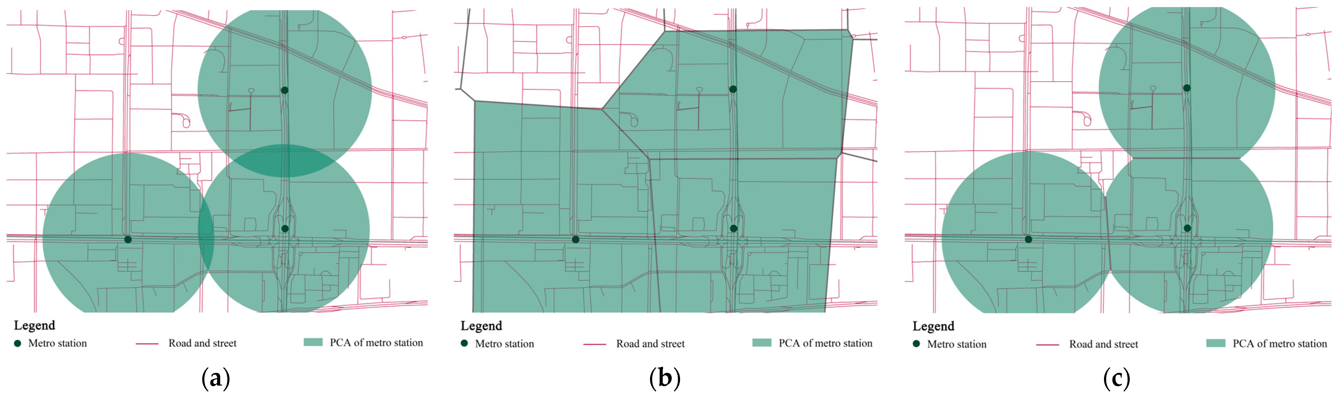
2.2. Delineation of PCA at Metro Stations

It is crucial to determine the scope of the built environment around metro stations before analyzing their influence on metro ridership. Due to the fact that the scope of this analysis is typically determined using the “maximum” walking distance or the area most users walk to [18,37], the scope of the built environment analysis around metro stations is commonly referred to as the pedestrian catchment area (PCA). The existing PCAs mainly consist of three types: circular buffer [8,13,18,23,24,30,31,33,34,38], Tyson polygon [39], and Tyson polygon superimposed with circular buffer [9,24,25,40] (Figure 1). However, considering the dense area of the metro stations, residents in the overlapping areas of the two stations may choose either of the stations. Therefore, we cannot determine which station they will choose. In order to simplify the processing and better determine the scope of the city’s TOD study [11], we have chosen circular buffers in this study. The radius of circular buffers selected by the existing studies is mostly 400 m [22], 500 m [13,31], 600 m [14,23,38], 800 m [8,10,18,24,33,40], and 1000 m [9,30]. The selection of buffer radius is mostly determined by pedestrian accessibility [17,23,33,40], experience [18], and reference to other research results [24]. In addition, in order to improve the accuracy of subway station PCA delineation, some scholars have proposed determining the PCA by goodness of fit. However, the radius of their alternative PCA was still determined by experience [9,14], and they often applied a unified PCA to all metro stations. However, the outskirts of super large cities like Beijing are mostly new areas with larger urban scales. Therefore, using the same PCA for metro stations in both new and old urban areas will reduce model accuracy. Meanwhile, previous research has demonstrated that partitioning metro stations is meaningful for enhancing model accuracy [11]. Although Andersson et al. and Wang et al. have categorized metro stations in the city [11,14], Andersson et al. [14] still adopted a unified PCA in the three zones in their study. In the study by Wang et al. [11], the two areas were analyzed independently. However, the model results may be biased because of the small number of metro stations in each zone. The metro stations in the city are divided into zones, and the candidate metro station PCA for each zone is determined based on the average station distance. Then, the PCA combination of the city is obtained, which can solve the limitations of the existing research. Currently, no scholars have determined the combined PCA of metro stations based on different areas.

2.3. Modeling Methods

Researchers worldwide have always been concerned with analyzing the influence of the constructed surroundings on subway ridership, and the methods for analyzing it are also rapidly advancing. The models used in the study included the Ordinary Least Squares (OLS) model [8,13,17,18,27,28,31,32], the Geographically Weighted Regression (GWR) model [14,24,29,33,41], the Two Stage Least Square (2SLS) model [29], and the Multi-Scale Geographically Weighted Regression (MGWR) model [9,23]. These linear models have been utilized by numerous scholars to investigate how the built environment affects metro ridership. However, the linear model is to be established on the premise of assuming the stationarity of the impact, which will lead to certain deviations in the analysis results [40]. The nonlinear model is considered an effective approach to solving this problem. Due to the rapid advancement of computer technology, it is possible to apply a variety of machine learning models. In current studies, random forest [42], deep learning [43,44], and Gradient Boosting Decision Trees (GBDT) [10,19,22] models are being used to analyze nonlinear relationships. However, these models have disadvantages, such as low accuracy and overfitting. eXtreme Gradient Boosting (XGBoost) is one of the most advanced machine learning algorithms at present. XGBoost has many advantages compared to other machine learning models: it prevents overfitting, is suitable for small data sets, responds to threshold effects, provides unified global interpretation and single sample interpretation, is not affected by multicollinearity, and can better handle outliers [45,46]. Currently, XGBoost has been widely utilized in prediction [47,48,49,50,51], smart city construction [52,53], remote sensing image processing [54], and other domains. Although some studies on metro ridership have utilized machine learning methods [10,19], they usually only use a single fixed machine learning method. However, the actual situation is that different data sets have different levels of precision with different models, so the validity of the models needs to be verified. Currently, there are few studies to verify the feasibility of modeling methods prior to modeling.

2.4. Current Gaps and Our Study

Combined with the existing research, we think that three deficiencies need to be solved. First of all, most existing studies do not partition metro stations and determine the combination of PCAs, which could potentially diminish the accuracy of the model, particularly in super-large cities like Beijing. Secondly, most existing studies directly choose a nonlinear model to investigate the impact of the built environment. Therefore, it may not be possible to determine the accuracy of the model in the specific dataset, which may bias the results. Finally, no station-level targeted strategies have been proposed in existing studies. This may not facilitate the implementation of subsequent strategies.
Therefore, we take boarding and deboarding ridership during the morning peak hours as the dependent variables. Thirteen explanatory variables of the built environment were selected as independent variables based on the “7D” dimension and the availability of big data. By evaluating the appropriateness of various PCA combinations across three different models, the study confirmed the most suitable model and identified the recommended PCA combinations for the three zones based on the model’s outcomes. The nonlinear effect of the built environment on metro ridership and the spatial heterogeneity of the impact are explored under the recommended PCA combination for the three zones. Finally, based on the study results, the metro stations with low vitality are identified, and the targeted strategy of the built environment is proposed.

3. Methods

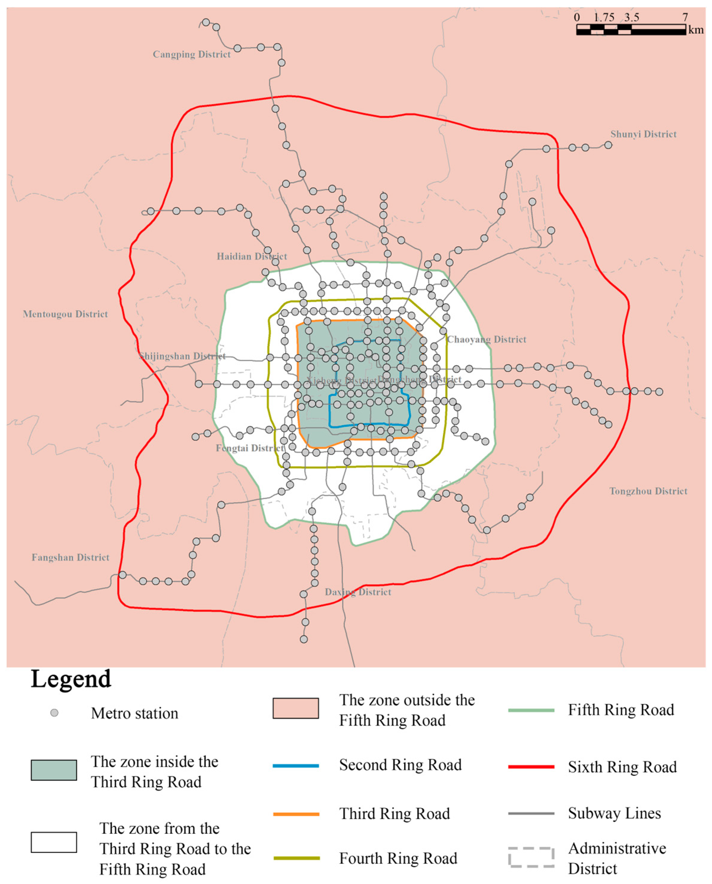
3.1. Study Scope and Data

Beijing is the representative of China’s megacities and is China’s political and cultural center. By 2020, Beijing’s metro mileage reached 689 km, ranking second in China and the world. Furthermore, as a result of the imbalance between supply and demand, certain metro stations are severely congested during morning peak hours. Therefore, Beijing is a good case study. Studying the complex relationship between metro ridership and the built environment in Beijing can provide the theoretical basis for metro construction, operation, and urban renewal in high-density cities in developing countries.
This study focuses on the 292 metro stations that have been put into service on the 19 metro lines that were in operation in Beijing by 2020 (compared with the metro operation stations published on the official website of Beijing Metro, the subway stations we selected have been in operation since 2020). We found that metro stations inside the 3rd ring are relatively clustered, those from the 3rd to the 5th ring are less clustered, and some of them are distributed parallel to the ring road, while those outside the 5th ring are more dispersed. Therefore, we categorized Beijing metro stations into three zones: inside the 3rd ring (green-filled area), from the 3rd to the 5th ring (white-filled area), and outside the 5th ring (pink-filled area) (Figure 2). Based on the bus IC card data, the average value of hourly boarding and deboarding ridership at each metro station during five working days from 12 October 2020 to 16 October 2020 in Beijing was obtained. The trend of boarding and deboarding ridership (Figure 3) indicates that the morning peak hours are from 7:00 to 9:00 and the evening peak hours are from 17:00 to 19:00. Since the conflict is more prominent during morning peak hours, this paper only analyses the relationship between the built environment and ridership during morning peak hours. The spatial distribution of the boarding ridership during the morning peak hours (hereafter referred to as boarding ridership) and the deboarding ridership during the morning peak hours (hereafter referred to as deboarding ridership) of metro stations are shown in Figure 4. In this study, we utilized the ridership of the metro station as a measure of the station’s vitality. In Figure 4, we divide the ridership into 5 levels using the natural break point method, and the stations at level 1 have lower vitality. The stations highlighted in red in Figure 4 indicate low vitality.

3.2. Explanatory Variable

The “7D” dimension consists of Density, Diversity, Design, Destination Accessibility, Distance to Transit, Demand Management, and Demographics [36]. We constructed 13 built environment explanatory variables based on the availability of big data and the “7D” dimension (see Table 2). The explanatory variables’ road network data, floor area, and bus lines data were obtained from OpenStreetMap (https://map.baidu.com, accessed on 10 October 2021). Points of interest (POI), car park, and bus stop data were obtained from the Golder API (https://lbs.amap.com, accessed on 10 October 2021). The data on underground station entrances and exits come from the official website of Beijing Subway (https://www.bjsubway.com, accessed on 13 October 2020). Population data were obtained from Worldpop (https://hub.worldpop.org, accessed on 10 October 2020). The population data in Worldpop is raster data, and we initially converted it into points. This is then intersected with the PCA of the metro station. If there are multiple population point data in a PCA, it is averaged.

3.3. Research Framework

This study is based on the availability of multi-source big data. It considers the influence of different PCA combinations and models on the results, determines the models and PCA combinations suitable for this study, and explores the effect of the built environment on metro ridership and spatial heterogeneity. The overall framework of this study is illustrated in Figure 5. Firstly, Beijing was segmented into three zones, and the PCA of each zone’s metro station was determined based on the average station distance of the three zones. Subsequently, 27 PCA combinations for the metro stations were identified. Secondly, 27 built environment datasets were created based on the 27 PCA combinations. Thirdly, six models—eXtreme Gradient Boosting (XGBoost), Light Gradient Boosting Machine (LightGBM), Random Forest (RF), Support Vector Machine (SVM), Gradient Boosting Decision Tree (GBDT), and Ordinary Least Squares (OLS)—were constructed using the morning peak hour boarding and deboarding ridership as dependent variables. By comparing the results of six models, the suitable models and PCA combinations for this study were determined. Finally, the study examined the impact of the built environment on metro ridership and spatial heterogeneity using appropriate models and PCA combinations. Furthermore, priority update metro stations were selected based on the morning peak hour boarding and deboarding ridership, and targeted urban renewal strategies are proposed. This study presents new ideas for implementing more accurate strategies to update the built environment around metro stations.

3.4. Delineation of PCA at Metro Stations

The delineation of the PCA affects the accuracy of the model [9,11], and the recommended PCA varies from city to city [55]. Therefore, the PCA recommended in this study should be determined before calculating the built environment variables. In order to enhance the accuracy of the model, our study aims to reduce the influence of the urban scale on the model results as much as possible. The average distances of metro stations inside the 3rd ring, from the 3rd to the 5th ring, and outside the 5th ring are 800 m, 1000 m, and 2000 m, respectively. In order to reduce the number of PCA combinations, it is convenient to carry out model statistical analysis. Add and subtract 200 m from the average distance of metro stations in each zone, so three circular buffers of different radii are set as PCAs for each zone. Therefore, a total of 27 PCA combinations were obtained to calculate the built environment explanatory variables of metro stations.

3.5. Machine Learning Models

3.5.1. eXtreme Gradient Boosting (XGBoost)

A gradient enhancement-based algorithm, XGBoost, was proposed by Chen et al. in 2016 [56]. The XGBoost algorithm reduces the residuals between the true and predicted values by constantly forming new regression trees to fit the previous prediction residuals [54]. This is one of the reasons for the high accuracy of XGBoost. Through a gradient-boosting framework and more controllability parameters, the XGBoost algorithm improves the algorithm’s problem-solving ability. In addition, XGBoost demonstrates good stability across different data processing methods [54].

3.5.2. Light Gradient Boosting Machine (LightGBM)

The LightGBM framework was proposed by Microsoft Research Asia (MSRA) in 2017 [57]. This algorithm is proposed to solve the issue of low learning efficiency for some models, such as GBDT and XGBoost, when dealing with large datasets. LightGBM is a histogram-based algorithm, so it has the advantages of smaller memory and faster training. However, LightGBM may grow deeper decision trees during model building, leading to overfitting.

3.5.3. Random Forest (RF)

RF, proposed by Leo Breiman in 2001 [58], is a typical Bagging algorithm in ensemble learning. Generally, a random forest is obtained by randomly combining free-growing CART decision trees and Bagging in a random subspace. RF has the advantages of high efficiency and good handling of missing values, but it is easy to overfit.

3.5.4. Support Vector Machines (SVM)

SVM was proposed by Cortes and Vapnik in 1995 [59]. Similar to logistics regression, SVM was originally based on a linear discriminant function with the help of convex optimization technology to solve the binary classification problem. However, unlike logistic regression, its output is classified by category, not category probability. The SVM algorithm has the advantage of being interpretable and suitable for small sample data, but it has the disadvantage of being difficult to train with large amounts of data.

3.5.5. Gradient Boosting Decision Trees (GBDT)

Gradient Boosting Decision Trees, also known as MART (Multiple Additive Regression Trees), are iterative algorithms that use decision trees. As a final prediction, this model aggregates the results of multiple decision trees constructed of weak learning trees. Decision trees and integration ideas are combined effectively in the algorithm. The GBDT model has the advantages of fast computation speed and strong interpretability, but it also has some disadvantages, such as easy overfitting.

3.6. Explanation of Machine Learning Models: Shapley Additive exPlanations (SHAP)

Machine learning models are commonly interpreted using SHAP, which is calculated as follows:
θ E = D E \ j D ! E D 1 ! E ! f D j x D j f D x D
where θ E is the Shapley value of variable E, D is a subset of the features incorporated into the model, and x D is the value vector of variable D. f D j x D j f D x D denotes the difference between the outputs of the two models. If θ E is calculated to be greater than 0, the feature is considered to positively influence the model prediction, and vice versa.

4. Results

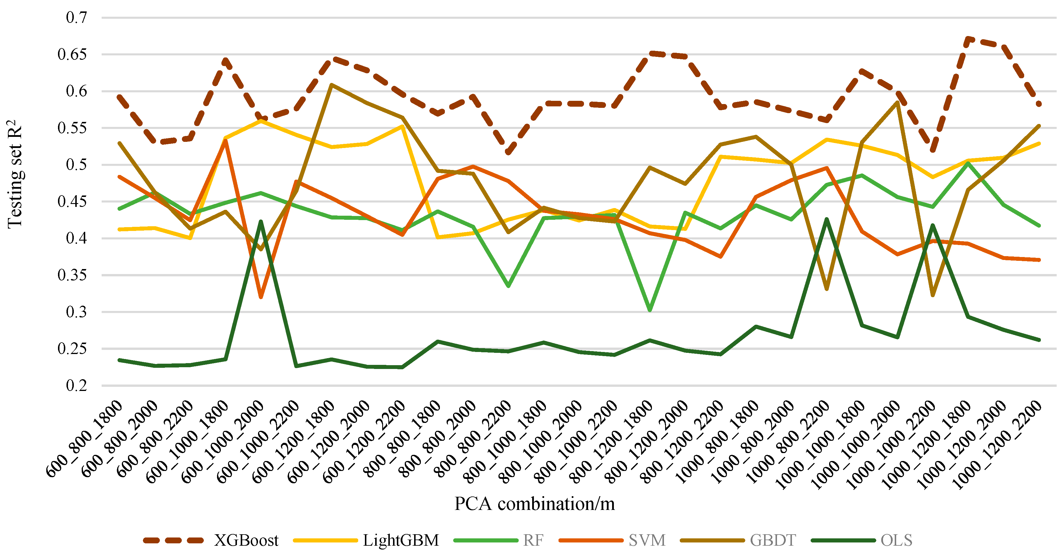
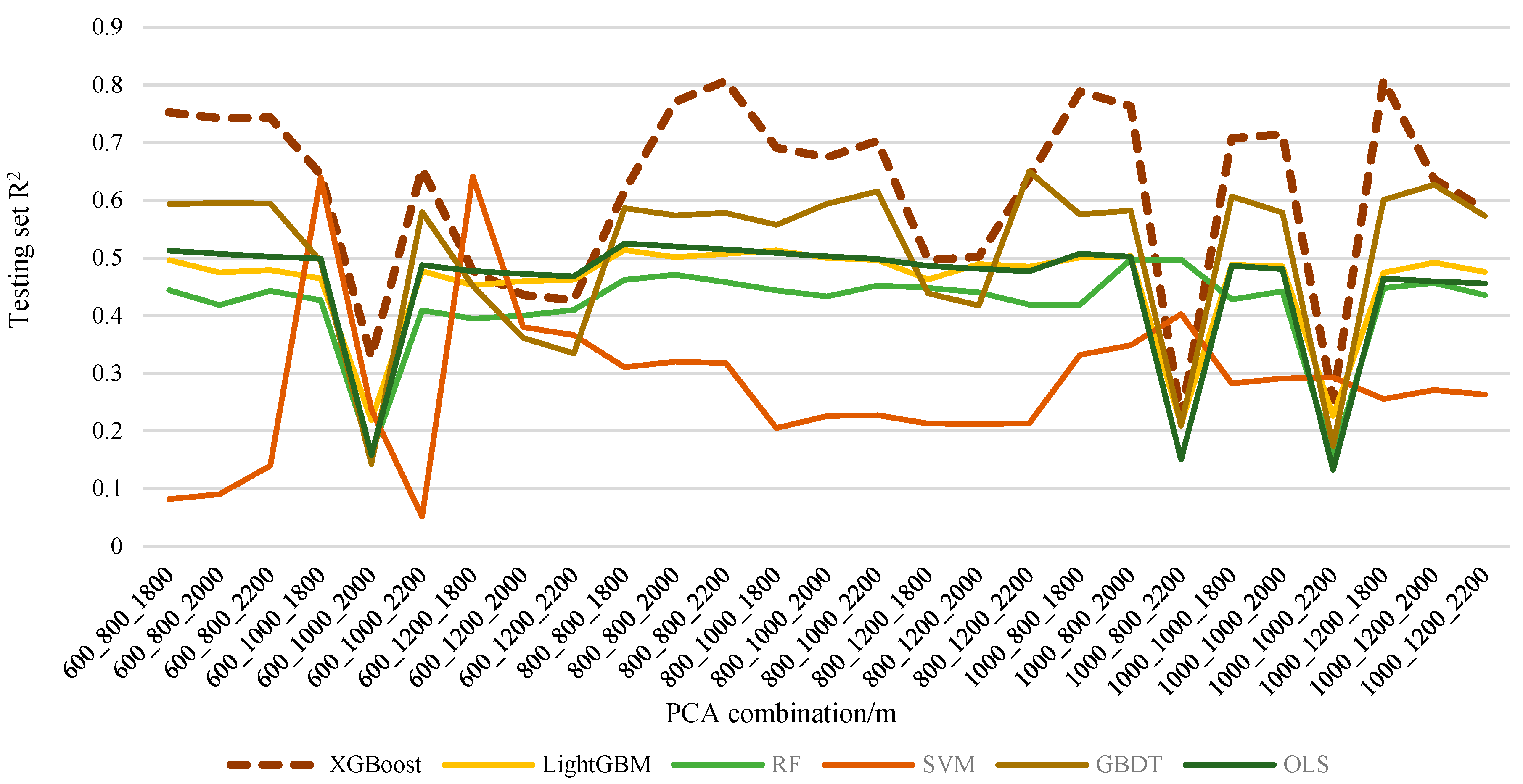
4.1. Model Performance and Recommended PCA Combinations

In order to identify an appropriate machine learning model for this study, we compared the coefficient of determination (R2) of the testing set of the XGBoost model with the R2 of the LightGBM, RF, SVM, GBDT, and OLS testing sets. The modeling results for boarding and deboarding ridership are shown in Figure 6 and Figure 7, respectively. The figure shows that for the same PCA combination, the R2 of XGBoost is larger than other models in general. This proves that the XGBoost model is more accurate than the traditional linear and machine learning models.
In addition, for the boarding ridership, when the combination of PCA is 1000 m_1200 m_1800 m (1000 m inside the 3rd ring, 1200 m from the 3rd to the 5th ring, and 1800 m outside the 5th ring), R2 is 0.67, which reaches the highest point. It is shown that the XGBoost model, under this PCA combination, has the highest goodness of fit. Therefore, the recommended PCA combination for analyzing boarding ridership is 1000 m_1200 m_1800 m. (Figure 6). For the deboarding ridership, when the PCA combination is 1000 m_1200 m_1800 m (1000 m inside the 3rd ring, 1200 m from the 3rd to the 5th ring, and 1800 m outside the 5th ring), the R2 is 0.81, which reaches the highest goodness of fit. Therefore, the recommended PCA combination for analyzing deboarding ridership is 1000 m_1200 m_1800 m. (Figure 7).

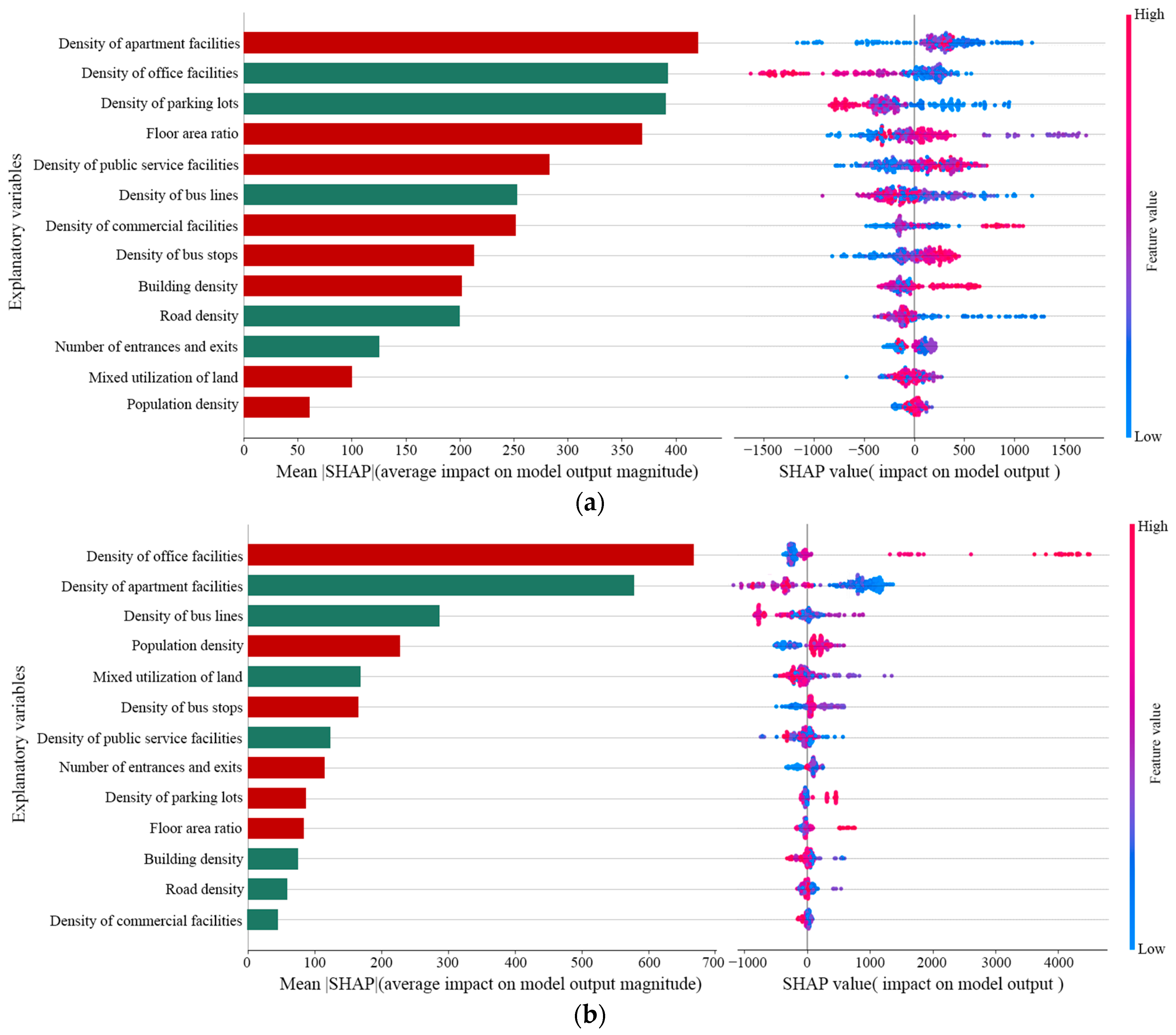
4.2. Relative Importance of the Impact of Explanatory Variables on Metro Ridership

To examine the influence of the independent variables in the recommended PCA combination, calculate the average of the absolute SHAP values for each independent variable from the results of the XGBoost model, and consider this as an indicator of the influence of the independent variables on metro ridership. A higher average of the absolute SHAP values indicates a stronger influence of the independent variables. The relative importance of the explanatory variables for boarding and deboarding ridership is shown in Figure 8. The left side of the figure shows the type of influence of the explanatory variables and the order of the explanatory variables. The red markers represent positive influence, while the green markers represent negative influence. The positive and negative impacts are judged based on the scatter plot located on the right side of the figure.
For boarding ridership, the explanatory variables have the following degree of influence: density of apartment facilities > density of office facilities > density of parking lots > floor area ratio > density of public service facilities > density of bus lines > density of commercial facilities > density of bus stops > building density > road density > number of entrances and exits > mixed utilization of land > population density (Figure 8a). At the same time, we find that among the explanatory variables given by the top three in the degree of influence, the density of apartment facilities has a positive influence. It proves that the larger the eigenvalue of the density of apartment facilities, the more significant the impact on boarding ridership. The density of office facilities and the density of parking lots have a negative impact on boarding ridership.
For deboarding ridership, the explanatory variables have the following degree of influence: density of office facilities > density of apartment facilities > density of bus lines > population density > mixed utilization of land > density of bus stops > density of public service facilities > number of entrances and exits > density of parking lots > floor area ratio > building density > road density > density of commercial facilities (Figure 8b). The density of apartment facilities, density of bus lines, mixed utilization of land, density of public service facilities, building density, road density, and density of commercial facilities have a negative impact on metro ridership, while the other explanatory variables have a positive impact on metro ridership. The density of office facilities among the top three in terms of the degree of influence has a positive effect, which proves that the larger the eigenvalue of this explanatory variable is, the greater the influence on metro ridership is. We compared the relative importance of the explanatory variables for boarding and deboarding ridership and found that the top two explanatory variables are the density of office and apartment facilities. These two variables have opposite positive and negative effects on ridership.

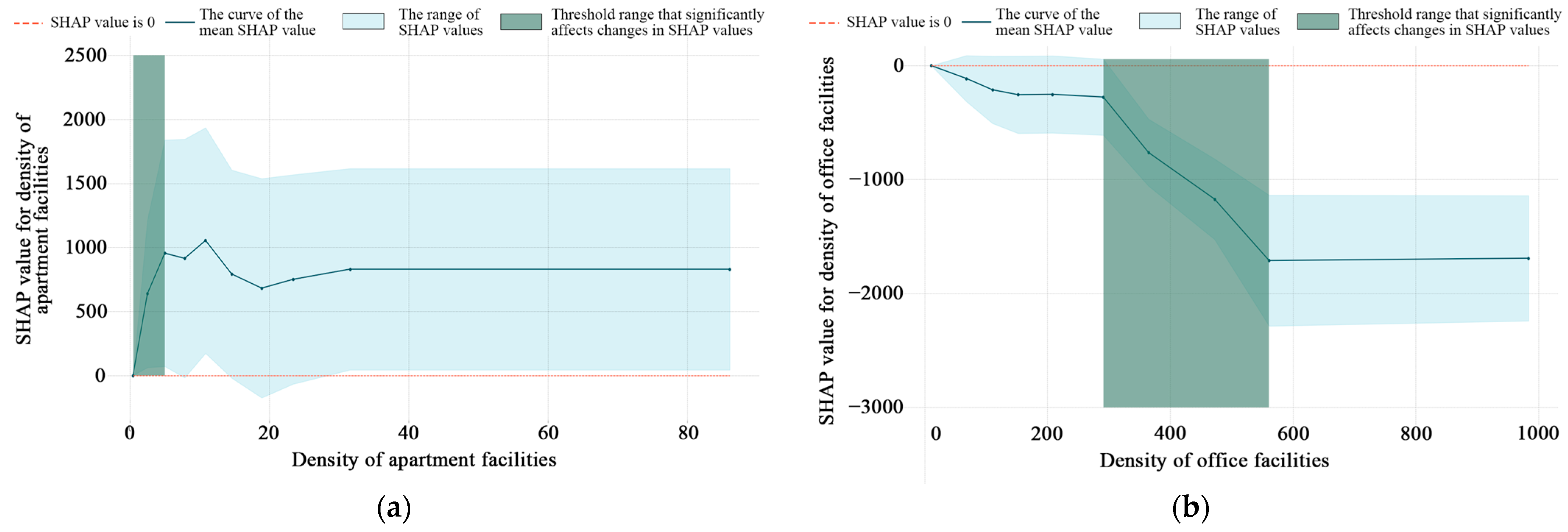
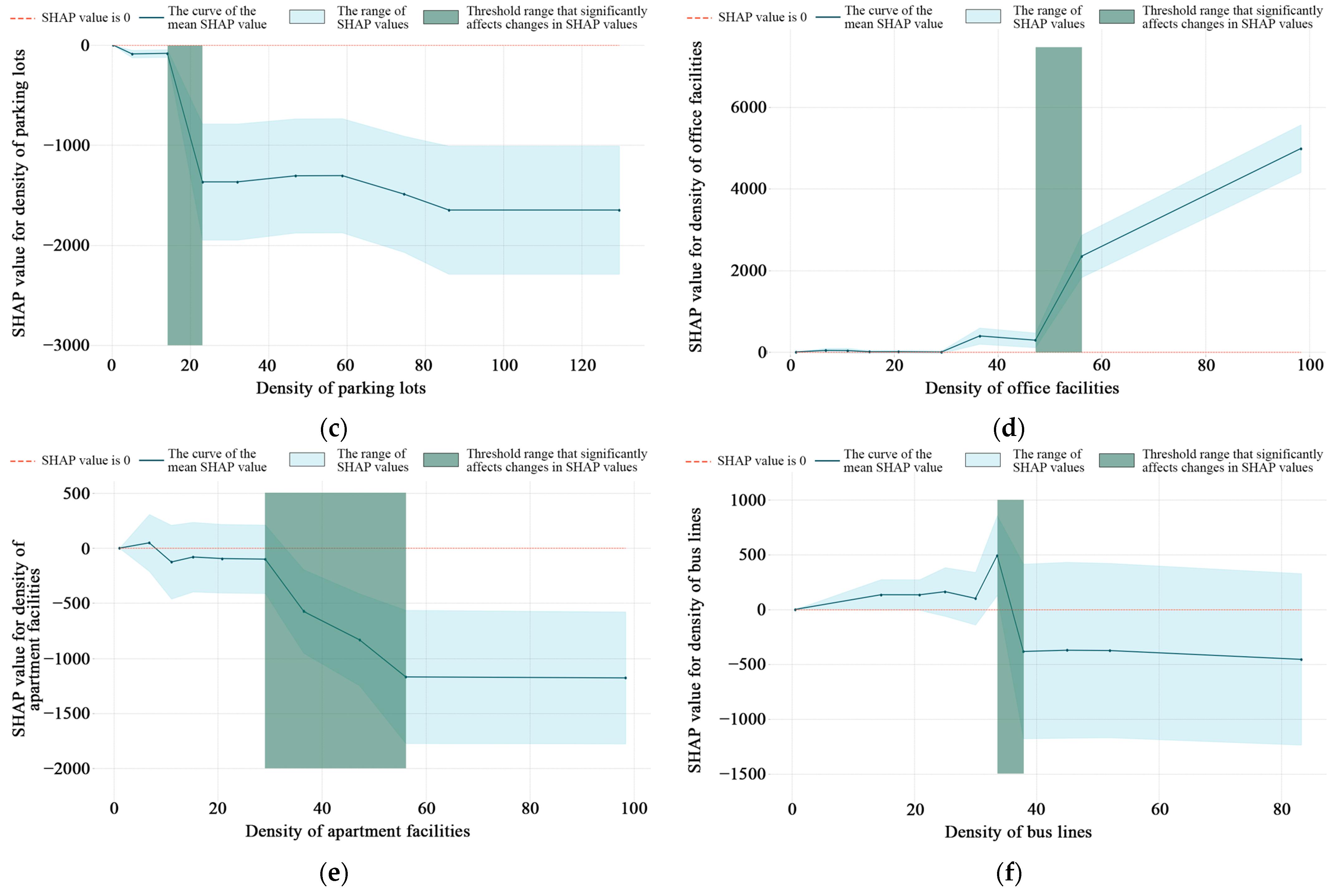
4.3. Threshold Effects of Explanatory Variables

Based on the results of the relative importance of the explanatory variables in Section 4.2, we selected the top three explanatory variables in terms of the degree of influence to analyze the threshold effect, and the results are shown in Figure 9. Overall, complex nonlinear relationships and threshold effects exist between our selected explanatory variables and metro ridership. There is an overall positive correlation between the density of apartment facilities and boarding ridership. There is residential segregation in Beijing, and many residents choose the metro to get to work. Therefore, there are more residential areas with a large ridership. The effect of the density of apartment facilities on ridership rises rapidly when the density of apartment facilities lies between 0 and 5 quantity/km2 (Figure 9a). This range is referred to as the threshold range that significantly influences changes in SHAP values, and we have labeled the threshold range for the explanatory variables in each figure with green markers. As for the density of apartment facilities, which is the most important variable affecting boarding ridership, we found that the higher density does not significantly impact ridership. The effect tends to be unchanged when the density of apartment facilities is greater than 32 quantity/km2. The possible reason is that when there are too many residential areas, the metro station becomes overloaded and is unable to accommodate increased ridership. The thresholds for the density of office facilities range from 300 to 550 quantity/km2, and the impact on ridership tends to be unchanged when the density of office facilities is greater than 550 quantity/km2 (Figure 9b). The possible reason is that the plot ratio for office land is typically high, and increasing the number of office land does not necessarily mean an increase in land area, so there is still available residential land. The threshold range of car park density is 15–22 quantity/km2, while its effect on ridership tends to be unchanged when the car park density is greater than 85 quantity/km2 (Figure 9c). The possible reason is that residents have a specific need for parking lots; if the demand exceeds it, the parking lots will become redundant.
For deboarding ridership, the effect of the density of office facilities on ridership increases with increasing eigenvalues and does not reach a leveling trend. This may be because office facilities are now more located in urban centers, with fewer residential facilities in these areas. Therefore, increasing the distribution of office facilities will always increase foot traffic. Meanwhile, the threshold range of the density of office facilities is 48–55 quantity/km2 (Figure 9d). When the density of apartment facilities and the density of bus lines reach 57 quantity/km2 and 38 km/km2, their impact on ridership tends to stabilize. The possible reason is that residents have a certain demand for public transport, so an unlimited increase in the number of public transport lines cannot increase ridership. Meanwhile, the threshold range for the density of apartment facilities was 30–55 quantity/km2 (Figure 9e), and the threshold range for the density of bus lines was 32–38 km/km2 (Figure 9f).
Comparing and analyzing the nonlinear results of boarding and deboarding ridership, we found that (1) except for the density of office facilities for deboarding ridership, all other variables ended up stabilizing their impact on metro ridership; (2) the nonlinear effects of the same variable on boarding and deboarding ridership vary widely, as do the threshold ranges, therefore, we need to study it based on the type of ridership; and (3) the two functions of living and working in a city significantly impact ridership. At the same time, the density of office and apartment facilities are the most critical factors affecting ridership, including both boarding and deboarding.

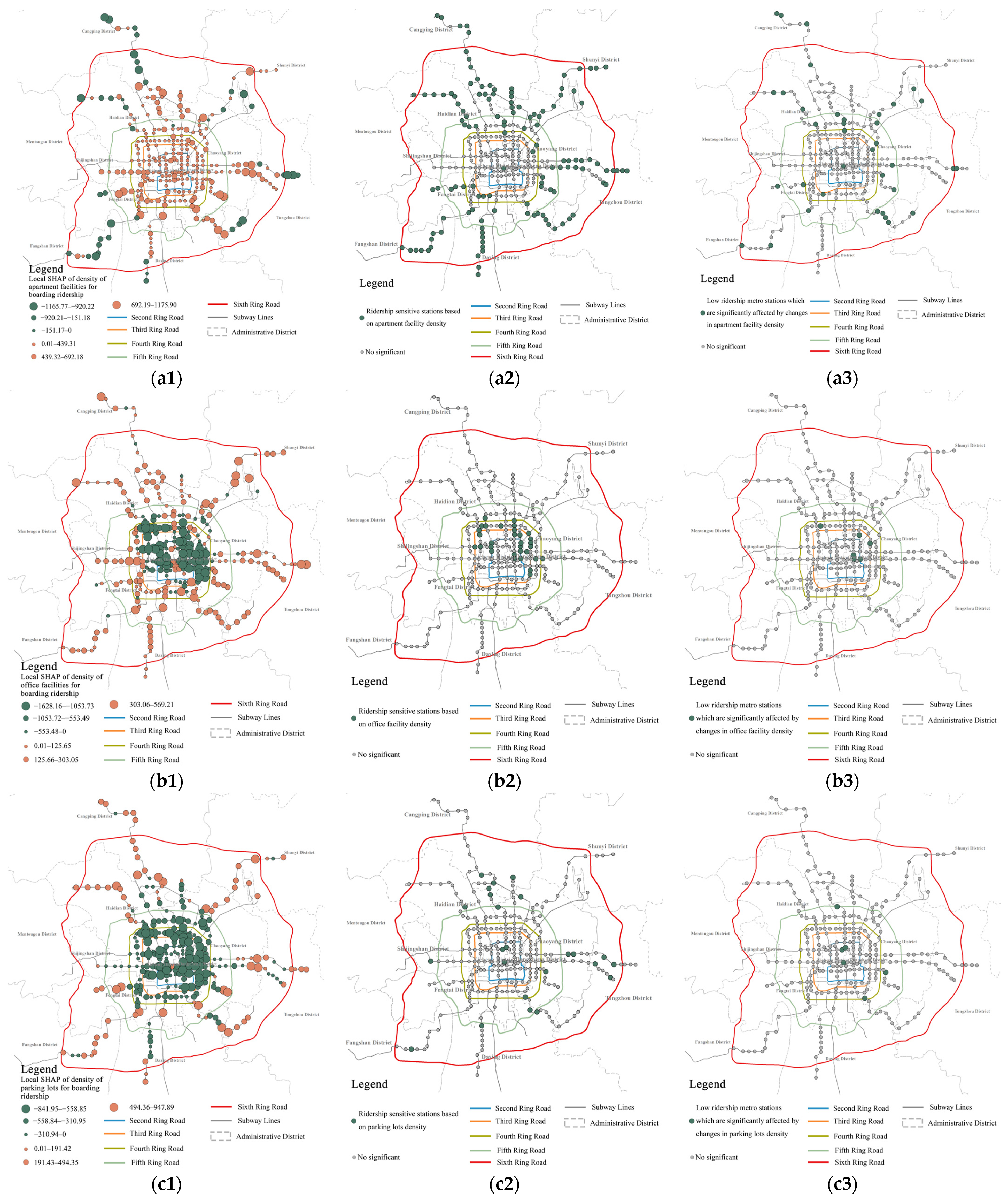
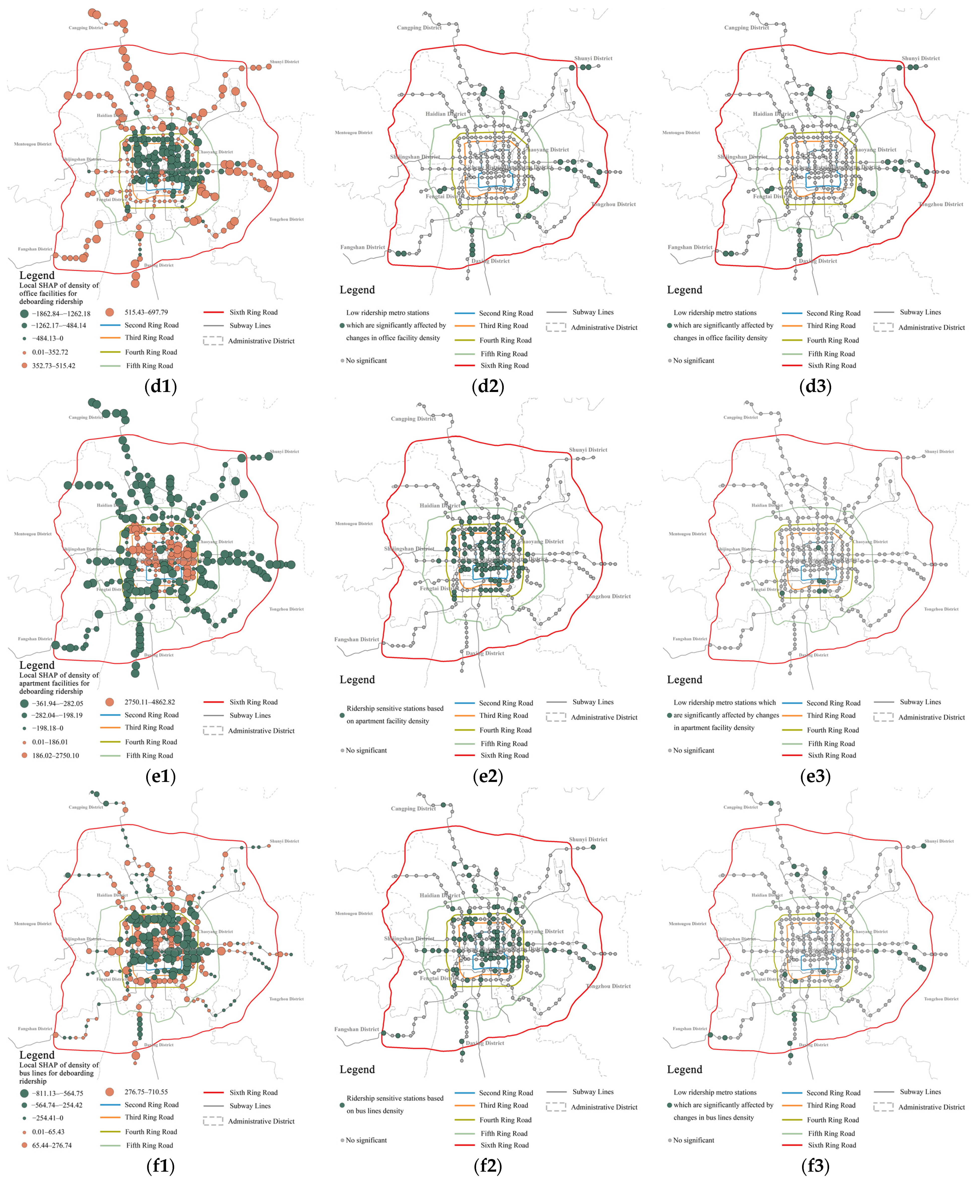
4.4. Spatial Heterogeneity in the Impact of Built Environment on Metro Ridership

According to the XGBoost model results, the SHAP values are classified by the natural break point method and visualized in ArcMap. For a station, if the value of the explanatory variable is in the threshold range that significantly affects the change in the SHAP value, we call this station a “ridership sensitive station based on the explanatory variable”. We visualized the locations of these sensitive stations in ArcMap to determine their distribution. In addition, we cross-analyzed the “ridership sensitive station based on the explanatory variable” and stations with low boarding and deboarding ridership (red-marked) stations (Figure 4). The chosen metro stations are the ones we need to update preferentially. It is also convenient to propose targeted strategies for renewing the built environment to enhance the vitality of metro stations.
For boarding ridership, the positive impact of the density of apartment facilities is concentrated in the interior areas, while the negative impact is concentrated in the exterior. Meanwhile, we found that all metro stations within the 5th ring are positively influenced (Figure 10(a1)). Figure 10(a2) shows the stations with ridership sensitivity based on the density of apartment facilities. Figure 10(a3) shows the prioritized stations for updating based on Figure 10(a2) and metro station ridership. Combined with Figure 10(a1), we find that these are mostly positive effects of the density of apartment facilities, and we can increase the distribution of apartment facilities around these stations to improve vitality. Stations that are positively affected by the density of office facilities are concentrated externally, while stations that are negatively affected by the density of office facilities are concentrated internally (Figure 10(b1)). Based on the density of apartment facilities, the ridership-sensitive stations are located inside the 4th ring (Figure 10(b2)). Figure 10(b3) shows the prioritized stations for renewal based on the ridership-sensitive stations and metro ridership in which the impact of the density of office facilities on ridership is negative, and we can reduce the density of office facilities and increase the density of apartment facilities simultaneously. The SHAP’s spatial distribution for parking lots is similar to the density of office facilities (Figure 10(c1)). Figure 10(c2) shows the ridership-sensitive stations based on the density of parking lots, and these stations are more dispersed outside the 4th ring. Fewer priority stations were selected based on the ridership-sensitive stations and metro ridership, all located within the 5th ring (Figure 10(c3)). Combined with Figure 10(c1), we can adjust the distribution of parking lots around these stations accordingly.
The stations where the density of office facilities positively affects the deboarding ridership are predominantly located on the city’s outskirts. In contrast, the negatively affected stations are mainly distributed in the city center (Figure 10(d1)). This proves the presence of job–housing separation in Beijing. The ridership-sensitive stations based on the density of apartment facilities are mainly located outside the 4th ring (Figure 10(d2)). Figure 10(d3) shows the metro stations selected based on ridership-sensitive stations and metro ridership. These stations are mainly located outside the 3rd Ring Road. It can be seen that the ridership of these stations is positively influenced by the density of office facilities. This demonstrates that we can opportunely increase the number of office facilities while reducing the number of other facilities around these stations during the later stages of urban renewal design. The SHAP value of the density of apartment facilities is opposite to that of the density of office facilities (Figure 10(e1)). Based on the density of apartment facilities, the ridership-sensitive stations are located inside the 4th ring (Figure 10(e2)). Fewer stations were chosen for priority renewal based on Figure 10(e2) and metro ridership (Figure 10(e3)). The positive and negative SHAP values of the density of bus lines are scattered within the study range, while stations with significant positive and negative values are mostly located within the 4th ring (Figure 10(f1)). Figure 10(f2) shows the ridership-sensitive stations based on the density of bus lines. For the priority update stations in Figure 10(f3), deboarding ridership can be adjusted based on SHAP values.
We compared the results for boarding and deboarding ridership and we found that (1) the density of apartment facilities has a more significant impact on boarding ridership. The density of office facilities has a more significant impact on deboarding ridership. At the same time, Beijing faces a substantial separation between residential and occupational areas, making it necessary to balance apartment and office facilities to adjust ridership. (2) Most of the stations prioritized for renewal based on the explanatory variables are located in the city’s outskirts, and a smaller proportion are located in the city’s center. This proves that the outskirts of the city still need to be prioritized.

4.5. Built Environment Renewal Strategies

In order to propose specific strategies for updating the built environment at priority stations, we analyzed these stations and their associated sensitive explanatory variables. The statistical results are presented in Table 3. In the table, “+” indicates that the built environment has a significant positive impact on the ridership of the station, while “−” indicates that the built environment has a significant negative impact on the ridership of the station. According to this table, we can propose a specific strategy to update the built environment for certain stations. For instance, Lincuiqiao Station can increase the residential facilities and reduce the number of stops to improve inbound activity at the station. Yancun East can enhance the vitality of the station by increasing the number of apartment facilities and extending the length of bus lines. For other priority sites requiring updates, corresponding strategies for updating the built environment can also be found in Table 3. The method used in this study can be utilized to identify priority sites for renewal and propose targeted strategies for the renewal of the built environment.

5. Discussion

5.1. Advantages of XGBoost Model in Metro Ridership Modeling

In this study, we compared the R2 of the XGBoost testing set for each PCA combination with the R2 of the LightGBM, SVM, RF, GBDT, and OLS models, respectively. We found that the R2 of the XGBoost model is higher than that of other models, indicating that the XGBoost model has a better modeling effect in capturing nonlinear relationships compared to the other models in this study. Most existing studies directly describe that the model’s goodness of fit is better. However, different data may be suitable for different models, and they have not conclusively demonstrated that the model in the paper is better [19,20,21,26,40,60,61]. This study solves the issue of the existing studies merely stating that using the model is better without providing evidence to support this claim. Although the XGBoost model has been compared with other models in existing studies [11], only the mean value of R2 was collected in their studies, and not all the results were shown. However, all the results from our research were presented, further substantiating the advantages of the XGBoost model. Furthermore, current studies emphasize the overfitting of models [26,40]. For example, Liu et al. [40] focused on the training set of models, while few scholars paid attention to the performance of the XGBoost model compared with other models.
Second, other machine learning methods cannot judge the positive and negative effects of the relative importance of explaining the variables as a whole [20,32]. However, the XGBoost model can visualize the results of each study object, resulting in the scatter plot in Section 4.2 of this study. We can judge the positive and negative effects of explanatory variables from the scatter plot. Urban planning decision-makers should consider not only the threshold effects of machine learning models and the results of spatial heterogeneity, but also the overall impact of explanatory variables. From an overall perspective, this makes it easier for us to increase ridership at fewer ridership stations. Furthermore, based on the threshold relationship of explanatory variables, this study can help us to identify the most effective range of different variables’ influence on ridership. In addition, by combining the threshold effect and ridership, we can identify the metro stations that should be prioritized for updates. At the same time, these stations are determined based on built explanatory variables that are sensitive to the impact of ridership, and the updated design for this built environment may be more conducive to improving the vitality of metro stations in the future. This provides a strong theoretical foundation for proposing targeted strategies in later stages. However, in previous studies [11,19,40], scholars typically did not classify stations after studying the spatial heterogeneity of the impact of explanatory variables, nor did they propose targeted improvement strategies. This makes the implementation of the research results very inconvenient.

5.2. Necessity of Using a PCA Combination of Metro Stations

The recommended PCA combination for analyzing boarding and deboarding ridership is 1000 m inside the 3rd ring, 1200 m from the 3rd to the 5th ring, and 1800 m outside the 5th ring. The results are consistent with our expectations, showing a higher PCA of metro stations located farther from the city center, which aligns with existing studies [11]. According to the results of this study, we suggest that the radius of the TOD ranges inside the 3rd ring, from the 3rd to the 5th ring, and outside the 5th ring in Beijing should be 1000 m, 1200 m, and 1800 m, respectively. In the study of Wang et al. [11], the city was divided into zones, and they found that the size of the PCA differed between the two city zones, and the degree of influence of the explanatory variables was not the same, which proved that the zoning should be based on the city’s development. However, they can reduce the amount of data by splitting the data, which can make the model less accurate. Currently, most studies use a unified PCA, and they choose a radius of 800 m [8,10,18,24,33,40]. This choice is primarily based on the widespread belief among scholars that 800 m is the maximum acceptable walking distance for residents. Some other scholars have used methods such as Tyson polygons, where each metro station has a different PCA [9,24,25,40]. This method can improve the model’s accuracy and avoid the city scale’s influence on the model results. However, this method cannot identify a universal PCA, which is not conducive to providing a basis for future research or determining the scope of TOD implementation in Beijing. And PCA combinations can help address the limitations in current studies. The R2 of our model with PCA combination is 0.81, which is higher than the R2 of Wang et al. [11]. It proves that the method of PCA combination can enhance the accuracy of the model.
In addition, to further demonstrate the necessity of using a PCA combination in this study, we compared the R2 of the XGBoost testing set of the unified metro PCA with the combined PCA, and the results are shown in Table 4. The results indicate that the R2 of the test set under the PCA combination is consistently higher than that of the unified PCA test set, regardless of boarding or deboarding ridership. This also proves that in this study, using a PCA combination can enhance the model’s accuracy, making it more suitable for the actual metro station services. The full sample data after the PCA combination improves the accuracy of classifying ridership and determining the threshold effect of explanatory variables. This makes the selected priority update stations more referential and the proposed targeted strategies more practical.

5.3. Comprehensive Analysis of the Influence of the Built Environment on Metro Ridership

For boarding and deboarding ridership, we found that the density of residential and office facilities had a more significant impact on ridership, consistent with our expected results and existing studies [8,9,13,23]. This result may be due to the fact that living and working are the two most important functions of a city. For commuters, living and working dominate, especially during weekday morning peak hours. In addition, this study found that the effect of the density of bus lines on ridership is negative and that the number of entrances and exits does not have a significant effect on ridership, which is inconsistent with the results of existing studies [8,30]. This result also proves that among those who choose to travel on the metro, fewer people take public transport to reach the metro station, while more people are likely to use bicycles and electric vehicles. In order to address the transportation needs in Beijing, it is essential to plan for more non-motorized car parks around metro stations. In particular, more shared bicycles need to be placed around metro stations with a high concentration of office buildings (e.g., Haidian District, which has a high volume of deboarding ridership). The minimal effect of the number of entrances and exits on ridership suggests that the characteristics of the Beijing metro station itself do not significantly affect ridership, which is primarily influenced by the surrounding built environment. The main reason for this is that ridership is generated by the amenities surrounding the metro stations, and the stations’ attributes do not affect ridership. This also proves that it is unreasonable to try to change the metro’s ridership by changing the metro station’s attributes, and it needs to be considered uniformly from the perspective of functional layout.
What is particularly interesting in this study is that the top two variables that greatly impact boarding and deboarding ridership are the density of apartment and office facilities. Their effects on the two types of ridership are opposite. This also proves that there is a relatively serious separation between employment and housing in Beijing, which is consistent with the findings of current research [11,62]. In addition, we found that the impact of the density of office facilities on deboarding ridership is different from that of the density of apartment facilities on deboarding ridership and the density of office and apartment facilities on boarding ridership, and it does not tend to be flat in the end. This proves that the more office facilities there are, the greater the impact on deboarding ridership. We suggest that the focus should be on improving apartment facilities to increase boarding ridership. However, according to the study results, it is not the case that a higher density of apartment facilities does not necessarily lead to better outcomes. Therefore, we also need to consider the nonlinear effects of the density of apartment facilities and try to stay within the sensitive threshold range. For increasing deboarding ridership, the focus should be on office facilities. Furthermore, metro stations located on the outskirts of cities typically experience lower numbers of passengers disembarking, whereas those situated in city centers generally have higher deboarding ridership. To sum up, we recommend that Beijing minimize the concentration of residential and office areas in one part of the city at the master planning level, and instead distribute these two functions in the city in a balanced way throughout the city. For example, creating a polycentric city could be a viable approach.

5.4. Strengths and Limitations

As far as we know, this study is the first to utilize a combination of PCAs to assess the scope of environmental analysis for subway station construction. The results show that this method can mitigate the impact of small data volume and the uniform effect of PCAs on model accuracy. Our study compared the XGBoost model with the OLS and other machine learning models before using it. The results demonstrated that the XGBoost model has a higher accuracy and is well suited for this study. This addresses the issue of some studies failing to verify the applicability of the XGBoost model before using it. Our study also utilized the results of the XGBoost model to identify subway stations that require priority updates, enabling the development of targeted construction environment update strategies. This addresses the issue of proposed strategies in studies that are not feasible to implement.
There are some limitations to this study. First, this study uses the average station distance between metro stations to determine the radius of potential PCAs and does not correct the reasonableness of the candidate radius based on actual Origin–Destination (OD) data. At the same time, the optimal PCA combination can be found by using the actual road network distance. Finally, our study did not utilize any land use data, which may have slightly impacted the model results.

6. Conclusions

The primary objective of this study is to identify the priority stations for renewal and propose targeted updating strategies. This study has the following contributions: (1) the accuracy of the XGBoost model is higher than that of the OLS and other machine learning models, and the XGBoost model is suitable for this study. (2) The model accuracy of different PCA combinations is different, and 1000 m_1200 m_1800 m is the PCA combination recommended in this study. (3) The priority metro stations for renewal are selected, and the countermeasures for the renewal of the built environment are put forward. The research framework of this study introduces a new approach for defining PCAs in metro stations and determining the TOD range in Beijing. At the same time, it also provides a valuable reference for putting forward the targeted strategy of built environment renewal.
Based on the study findings, the following recommendations are made: (1) it is recommended that when considering the scope of TOD in Beijing, the circular buffer with a radius of 1000 m should be considered inside the 3rd ring, the circular buffer with a radius of 1200 m from the 3rd to the 5th ring, and the circular buffer with a radius of 1800 m outside the 5th ring. (2) There is a need to focus on apartment and office facilities from a master planning perspective. It is possible to decongest some of the offices from the city center to the outskirts, particularly those with non-essential functions, and to develop polycentric cities. (3) Based on the ridership data and nonlinear threshold data, we have identified certain stations for priority updating. This allows us to implement targeted updating strategies for these stations.

Author Contributions

Conceptualization, Z.W., Y.Z., X.W. and D.L.; data curation, S.L. (Shihao Li) and S.L. (Shuyue Liu); funding acquisition, Y.Z. and X.W.; investigation, S.L. (Shihao Li); methodology, Z.W. and S.L. (Shuyue Liu); project administration, Y.Z.; software, D.L.; visualization, X.W.; writing—original draft, Z.W. and S.L. (Shihao Li); writing—review and editing, Z.W. and S.L. (Shihao Li). All authors have read and agreed to the published version of the manuscript.

Funding

This research was funded by the Hebei Social Science Development Research Project in 2023, China (grant No. 20230203044).

Institutional Review Board Statement

Not applicable.

Informed Consent Statement

Not applicable.

Data Availability Statement

The data used in this study are available from the corresponding author upon reasonable request.

Conflicts of Interest

The authors declare no conflicts of interest.

References

  1. Cullinane, S. The relationship between car ownership and public transport provision: A case study of Hong Kong. Transp. Policy 2002, 9, 29–39. [Google Scholar] [CrossRef]
  2. Goodwin, P.B. Car ownership and public transport use: Revisiting the interaction. Transportation 1993, 20, 21–33. [Google Scholar] [CrossRef]
  3. Nguyen-Phuoc, D.Q.; Currie, G.; De Gruyter, C.; Young, W. Congestion relief and public transport: An enhanced method using disaggregate mode shift evidence. Case Stud. Transp. Policy 2018, 6, 518–528. [Google Scholar] [CrossRef]
  4. Badland, H.M.; Rachele, J.N.; Roberts, R.; Giles-Corti, B. Creating and applying public transport indicators to test pathways of behaviours and health through an urban transport framework. J. Transp. Health 2017, 4, 208–215. [Google Scholar] [CrossRef]
  5. Cervero, R.; Day, J. Suburbanization and transit-oriented development in China. Transp. Policy 2008, 15, 315–323. [Google Scholar] [CrossRef]
  6. Shen, Q.; Chen, P.; Pan, H. Factors affecting car ownership and mode choice in rail transit-supported suburbs of a large Chinese city. Transp. Res. Part A Policy Pract. 2016, 94, 31–44. [Google Scholar] [CrossRef]
  7. News, C.E. The Results of the Fifth Comprehensive Traffic Survey in Beijing Were Announced. Available online: http://epaper.cenews.com.cn/html/2016-07/14/content_47058.htm (accessed on 18 November 2023).
  8. Zhao, J.; Deng, W.; Song, Y.; Zhu, Y. Analysis of Metro ridership at station level and station-to-station level in Nanjing: An approach based on direct demand models. Transportation 2013, 41, 133–155. [Google Scholar] [CrossRef]
  9. Wang, Z.; Song, J.; Zhang, Y.; Li, S.; Jia, J.; Song, C. Spatial Heterogeneity Analysis for Influencing Factors of Outbound Ridership of Subway Stations Considering the Optimal Scale Range of “7D” Built Environments. Sustainability 2022, 14, 16314. [Google Scholar] [CrossRef]
  10. Gan, Z.; Yang, M.; Feng, T.; Timmermans, H.J.P. Examining the relationship between built environment and metro ridership at station-to-station level. Transp. Res. Part D Transp. Environ. 2020, 82, 102332. [Google Scholar] [CrossRef]
  11. Wang, Z.; Li, S.; Li, Y.; Liu, D.; Liu, S.; Chen, N. Investigating the Nonlinear Effect of Built Environment Factors on Metro Station-Level Ridership under Optimal Pedestrian Catchment Areas via the Machine Learning Method. Appl. Sci. 2023, 13, 12210. [Google Scholar] [CrossRef]
  12. Chiang, W.-C.; Russell, R.A.; Urban, T.L. Forecasting ridership for a metropolitan transit authority. Transp. Res. Part A Policy Pract. 2011, 45, 696–705. [Google Scholar] [CrossRef]
  13. Sohn, K.; Shim, H. Factors generating boardings at Metro stations in the Seoul metropolitan area. Cities 2010, 27, 358–368. [Google Scholar] [CrossRef]
  14. Andersson, D.E.; Shyr, O.F.; Yang, J. Neighbourhood effects on station-level transit use: Evidence from the Taipei metro. J. Transp. Geogr. 2021, 94, 103127. [Google Scholar] [CrossRef]
  15. Fotheringham, A.S.; Yang, W.; Kang, W. Multiscale Geographically Weighted Regression (MGWR). Ann. Am. Assoc. Geogr. 2017, 107, 1247–1265. [Google Scholar] [CrossRef]
  16. Yu, H.; Fotheringham, A.S.; Li, Z.; Oshan, T.; Kang, W.; Wolf, L.J. Inference in Multiscale Geographically Weighted Regression. Geogr. Anal. 2019, 52, 87–106. [Google Scholar] [CrossRef]
  17. Zhao, J.; Deng, W. Relationship of Walk Access Distance to Rapid Rail Transit Stations with Personal Characteristics and Station Context. J. Urban Plan. Dev. 2013, 139, 311–321. [Google Scholar] [CrossRef]
  18. Zhao, J.; Deng, W.; Song, Y.; Zhu, Y. What influences Metro station ridership in China? Insights from Nanjing. Cities 2013, 35, 114–124. [Google Scholar] [CrossRef]
  19. Du, Q.; Zhou, Y.; Huang, Y.; Wang, Y.; Bai, L. Spatiotemporal exploration of the non-linear impacts of accessibility on metro ridership. J. Transp. Geogr. 2022, 102, 103380. [Google Scholar] [CrossRef]
  20. Ji, S.; Wang, X.; Lyu, T.; Liu, X.; Wang, Y.; Heinen, E.; Sun, Z. Understanding cycling distance according to the prediction of the XGBoost and the interpretation of SHAP: A non-linear and interaction effect analysis. J. Transp. Geogr. 2022, 103, 103414. [Google Scholar] [CrossRef]
  21. Caigang, Z.; Shaoying, L.; Zhangzhi, T.; Feng, G.; Zhifeng, W. Nonlinear and threshold effects of traffic condition and built environment on dockless bike sharing at street level. J. Transp. Geogr. 2022, 102, 103375. [Google Scholar] [CrossRef]
  22. Ding, C.; Cao, X.; Liu, C. How does the station-area built environment influence Metrorail ridership? Using gradient boosting decision trees to identify non-linear thresholds. J. Transp. Geogr. 2019, 77, 70–78. [Google Scholar] [CrossRef]
  23. Jun, M.-J.; Choi, K.; Jeong, J.-E.; Kwon, K.-H.; Kim, H.-J. Land use characteristics of subway catchment areas and their influence on subway ridership in Seoul. J. Transp. Geogr. 2015, 48, 30–40. [Google Scholar] [CrossRef]
  24. Li, S.; Lyu, D.; Huang, G.; Zhang, X.; Gao, F.; Chen, Y.; Liu, X. Spatially varying impacts of built environment factors on rail transit ridership at station level: A case study in Guangzhou, China. J. Transp. Geogr. 2020, 82, 102631. [Google Scholar] [CrossRef]
  25. Li, S.; Lyu, D.; Liu, X.; Tan, Z.; Gao, F.; Huang, G.; Wu, Z. The varying patterns of rail transit ridership and their relationships with fine-scale built environment factors: Big data analytics from Guangzhou. Cities 2020, 99, 102580. [Google Scholar] [CrossRef]
  26. Zhou, S.; Liu, Z.; Wang, M.; Gan, W.; Zhao, Z.; Wu, Z. Impacts of building configurations on urban stormwater management at a block scale using XGBoost. Sustain. Cities Soc. 2022, 87, 104235. [Google Scholar] [CrossRef]
  27. Gutiérrez, J.; Cardozo, O.D.; García-Palomares, J.C. Transit ridership forecasting at station level: An approach based on distance-decay weighted regression. J. Transp. Geogr. 2011, 19, 1081–1092. [Google Scholar] [CrossRef]
  28. Thompson, G.; Brown, J.; Bhattacharya, T. What Really Matters for Increasing Transit Ridership: Understanding the Determinants of Transit Ridership Demand in Broward County, Florida. Urban Stud. 2012, 49, 3327–3345. [Google Scholar] [CrossRef]
  29. Calvo, F.; Eboli, L.; Forciniti, C.; Mazzulla, G. Factors influencing trip generation on metro system in Madrid (Spain). Transp. Res. Part D Transp. Environ. 2019, 67, 156–172. [Google Scholar] [CrossRef]
  30. Sung, H.; Choi, K.; Lee, S.; Cheon, S. Exploring the impacts of land use by service coverage and station-level accessibility on rail transit ridership. J. Transp. Geogr. 2014, 36, 134–140. [Google Scholar] [CrossRef]
  31. Sung, H.; Oh, J.-T. Transit-oriented development in a high-density city: Identifying its association with transit ridership in Seoul, Korea. Cities 2011, 28, 70–82. [Google Scholar] [CrossRef]
  32. Loo, B.P.Y.; Chen, C.; Chan, E.T.H. Rail-based transit-oriented development: Lessons from New York City and Hong Kong. Landsc. Urban Plan. 2010, 97, 202–212. [Google Scholar] [CrossRef]
  33. Cardozo, O.D.; García-Palomares, J.C.; Gutiérrez, J. Application of geographically weighted regression to the direct forecasting of transit ridership at station-level. Appl. Geogr. 2012, 34, 548–558. [Google Scholar] [CrossRef]
  34. Estupiñán, N.; Rodríguez, D.A. The relationship between urban form and station boardings for Bogotá’s BRT. Transp. Res. Part A Policy Pract. 2008, 42, 296–306. [Google Scholar] [CrossRef]
  35. Ewing, R.; Cervero, R. Travel and the Built Environment. J. Am. Plan. Assoc. 2010, 76, 265–294. [Google Scholar] [CrossRef]
  36. De Gruyter, C.; Saghapour, T.; Ma, L.; Dodson, J. How does the built environment affect transit use by train, tram and bus? J. Transp. Land Use 2020, 13, 625–650. [Google Scholar] [CrossRef]
  37. Jiang, Y.; Christopher Zegras, P.; Mehndiratta, S. Walk the line: Station context, corridor type and bus rapid transit walk access in Jinan, China. J. Transp. Geogr. 2012, 20, 1–14. [Google Scholar] [CrossRef]
  38. Liu, J.; Wang, B.; Xiao, L. Non-linear associations between built environment and active travel for working and shopping: An extreme gradient boosting approach. J. Transp. Geogr. 2021, 92, 103034. [Google Scholar] [CrossRef]
  39. Sun, L.S.; Wang, S.W.; Yao, L.Y.; Rong, J.; Ma, J.M. Estimation of transit ridership based on spatial analysis and precise land use data. Transp. Lett. 2016, 8, 140–147. [Google Scholar] [CrossRef]
  40. Liu, M.; Liu, Y.; Ye, Y. Nonlinear effects of built environment features on metro ridership: An integrated exploration with machine learning considering spatial heterogeneity. Sustain. Cities Soc. 2023, 95, 104613. [Google Scholar] [CrossRef]
  41. Lu, B.; Yang, W.; Ge, Y.; Harris, P. Improvements to the calibration of a geographically weighted regression with parameter-specific distance metrics and bandwidths. Comput. Environ. Urban Syst. 2018, 71, 41–57. [Google Scholar] [CrossRef]
  42. Cheng, L.; Chen, X.; De Vos, J.; Lai, X.; Witlox, F. Applying a random forest method approach to model travel mode choice behavior. Travel Behav. Soc. 2019, 14, 1–10. [Google Scholar] [CrossRef]
  43. Hagenauer, J.; Helbich, M. A comparative study of machine learning classifiers for modeling travel mode choice. Expert Syst. Appl. 2017, 78, 273–282. [Google Scholar] [CrossRef]
  44. Zhao, X.; Yan, X.; Yu, A.; Van Hentenryck, P. Prediction and behavioral analysis of travel mode choice: A comparison of machine learning and logit models. Travel Behav. Soc. 2020, 20, 22–35. [Google Scholar] [CrossRef]
  45. Liang, W.; Luo, S.; Zhao, G.; Wu, H. Predicting Hard Rock Pillar Stability Using GBDT, XGBoost, and LightGBM Algorithms. Mathematics 2020, 8, 765. [Google Scholar] [CrossRef]
  46. Feng, D.C.; Wang, W.J.; Mangalathu, S.; Taciroglu, E. Interpretable XGBoost-SHAP Machine-Learning Model for Shear Strength Prediction of Squat RC Walls. J. Struct. Eng. 2021, 147, 04021173. [Google Scholar] [CrossRef]
  47. Sun, B.; Sun, T.; Jiao, P.; Tang, J. Spatio-Temporal Segmented Traffic Flow Prediction with ANPRS Data Based on Improved XGBoost. J. Adv. Transp. 2021, 2021, 5559562. [Google Scholar] [CrossRef]
  48. Ran, D.; Jiaxin, H.; Yuzhe, H. Application of a Combined Model based on K-means++ and XGBoost in Traffic Congestion Prediction. In Proceedings of the 2020 5th International Conference on Smart Grid and Electrical Automation (ICSGEA), Zhangjiajie, China, 13–14 June 2020; pp. 413–418. [Google Scholar]
  49. Lv, C.X.; An, S.Y.; Qiao, B.J.; Wu, W. Time series analysis of hemorrhagic fever with renal syndrome in mainland China by using an XGBoost forecasting model. BMC Infect. Dis 2021, 21, 839. [Google Scholar] [CrossRef] [PubMed]
  50. Tang, J.; Zheng, L.; Han, C.; Liu, F.; Cai, J. Traffic Incident Clearance Time Prediction and Influencing Factor Analysis Using Extreme Gradient Boosting Model. J. Adv. Transp. 2020, 2020, 6401082. [Google Scholar] [CrossRef]
  51. Ma, M.; Zhao, G.; He, B.; Li, Q.; Dong, H.; Wang, S.; Wang, Z. XGBoost-based method for flash flood risk assessment. J. Hydrol. 2021, 598, 126382. [Google Scholar] [CrossRef]
  52. Le, L.T.; Nguyen, H.; Zhou, J.; Dou, J.; Moayedi, H. Estimating the Heating Load of Buildings for Smart City Planning Using a Novel Artificial Intelligence Technique PSO-XGBoost. Appl. Sci. 2019, 9, 2714. [Google Scholar] [CrossRef]
  53. Garcia-Retuerta, D.; Chamoso, P.; Hernández, G.; Guzmán, A.S.R.; Yigitcanlar, T.; Corchado, J.M. An Efficient Management Platform for Developing Smart Cities: Solution for Real-Time and Future Crowd Detection. Electronics 2021, 10, 765. [Google Scholar] [CrossRef]
  54. Zhao, D.; Zhen, J.; Zhang, Y.; Miao, J.; Shen, Z.; Jiang, X.; Wang, J.; Jiang, J.; Tang, Y.; Wu, G.; et al. Mapping mangrove leaf area index (LAI) by combining remote sensing images with PROSAIL-D and XGBoost methods. Remote Sens. Ecol. Conserv. 2022, 9, 370–389. [Google Scholar] [CrossRef]
  55. Guerra, E.; Cervero, R.; Tischler, D. Half-Mile Circle. Transp. Res. Rec. J. Transp. Res. Board 2012, 2276, 101–109. [Google Scholar] [CrossRef]
  56. Chen, T.; Guestrin, C. XGBoost: A Scalable Tree Boosting System. In Proceedings of the 22nd ACM SIGKDD International Conference on Knowledge Discovery and Data Mining, San Francisco, CA, USA, 13–17 August 2016; pp. 785–794. [Google Scholar]
  57. Hajihosseinlou, M.; Maghsoudi, A.; Ghezelbash, R. A Novel Scheme for Mapping of MVT-Type Pb-Zn Prospectivity: LightGBM, a Highly Efficient Gradient Boosting Decision Tree Machine Learning Algorithm. Nat. Resour. Res. 2023, 32, 2417–2438. [Google Scholar] [CrossRef]
  58. Breiman, L. Random forests. Mach. Learn. 2001, 45, 5–32. [Google Scholar] [CrossRef]
  59. Cortes, C.; Vapnik, V. Support-vector networks. Mach. Learn. 1995, 20, 273–297. [Google Scholar] [CrossRef]
  60. Kim, S.; Lee, S. Nonlinear relationships and interaction effects of an urban environment on crime incidence: Application of urban big data and an interpretable machine learning method. Sustain. Cities Soc. 2023, 91, 104419. [Google Scholar] [CrossRef]
  61. Yang, C.; Chen, M.; Yuan, Q. The application of XGBoost and SHAP to examining the factors in freight truck-related crashes: An exploratory analysis. Accid. Anal. Prev. 2021, 158, 106153. [Google Scholar] [CrossRef]
  62. Liu, Y.; Yao, G.; Cai, C.; Cui, K. Job-Housing Spatial Distribution and the Commuting Characteristics in Beijing. Urban Transp. China 2022, 20, 98–104. [Google Scholar] [CrossRef]
Figure 1. Three PCA delineation methods: (a) circular buffer; (b) Tyson polygon; (c) Tyson polygon superimposed with circular buffer.
Sustainability 16 01178 g001
Figure 2. Metro station zoning.
Sustainability 16 01178 g002
Figure 3. Hourly variation in boarding and deboarding ridership of metro stations on weekdays.
Sustainability 16 01178 g003
Figure 4. Spatial distribution of metro ridership during the morning peak hours: (a) boarding ridership and (b) deboarding ridership.
Sustainability 16 01178 g004
Figure 5. Analytical framework.
Sustainability 16 01178 g005
Figure 6. Comparison of R2 for different models of boarding ridership.
Sustainability 16 01178 g006
Figure 7. Comparison of R2 for different models of deboarding ridership.
Sustainability 16 01178 g007
Figure 8. Relative importance of explanatory variables: (a) boarding ridership and (b) deboarding ridership.
Sustainability 16 01178 g008
Figure 9. Nonlinear results for explanatory variables of boarding and deboarding ridership: (a) density of apartment facilities for boarding ridership; (b) density of office facilities for boarding ridership; (c) density of parking lots for boarding ridership; (d) density of office facilities for deboarding ridership; (e) density of apartment facilities for deboarding ridership; and (f) density of bus lines for deboarding ridership.
Sustainability 16 01178 g009aSustainability 16 01178 g009b
Figure 10. A map of the spatial distribution of the SHAP values of the environmental explanatory variables and a map of the prioritized update sites were constructed: (a1) SHAP of the density of apartment facilities for boarding ridership; (a2) ridership-sensitive stations based on the density of apartment facilities for boarding ridership; (a3) intersection of low ridership stations and sensitive stations based on the density of apartment facilities for boarding ridership and boarding ridership; (b1) SHAP of the density of office facilities for boarding ridership; (b2) ridership-sensitive stations based on the density of office facilities for boarding ridership; (b3) intersection of low-ridership stations and sensitive stations based on the density of office facilities for boarding ridership and boarding ridership; (c1) SHAP of the density of parking lots for boarding ridership; (c2) ridership-sensitive stations based on the density of parking lots for boarding ridership; (c3) intersection of low-ridership stations and sensitive stations based on the density of parking lots for boarding ridership and boarding ridership; (d1) SHAP of the density of office facilities for deboarding ridership; (d2) ridership-sensitive stations based on the density of office facilities for deboarding ridership; (d3) intersection of low-ridership stations and sensitive stations based on the density of office facilities for deboarding ridership and deboarding ridership; (e1) SHAP of the density of apartment facilities for deboarding ridership; (e2) ridership-sensitive stations based on the density of apartment facilities for deboarding ridership; (e3) intersection of low-ridership stations and sensitive stations based on the density of apartment facilities for deboarding ridership and deboarding ridership; (f1) SHAP of the density of bus lines for deboarding ridership; (f2) ridership-sensitive stations based on the density of bus lines for deboarding ridership; (f3) intersection of low-ridership stations and sensitive stations based on the density of bus lines for deboarding ridership and deboarding ridership.
Sustainability 16 01178 g010aSustainability 16 01178 g010b
Table 1. Explanatory variables of different literatures were selected and compared.
Explanatory VariablesEstupiñán et al. (2008) [34] Sohn et al. (2010) [13] Loo et al. (2010) [32]Gutiérrez et al. (2011) [27]Sung et al. (2011) [31]Cardozo et al. (2012) [33]Zhao et al. (2013) [18]Zhao et al. (2013) [8]Hyungun et al. (2014) [30]Jun et al. (2015) [23]Calvo et al. (2019) [29]Ding et al. (2019) [22]Li et al. (2020) [24]Gan et al. (2020) [10] Andersson et al. (2021) [14]Wang et al. (2022) [9]Du et al. (2022) [19]
Land use and densityEmployment density
Commercial/residential building area or density
Land use mixing degree
Off-street parking area
Floor area ratio
Number and density of hotels/restaurants/hospitals/universities
AccessibilityAverage walking distance from residence
Distance from city centre or CBD
Perceived attributes (safety, convenience, cycling, and walking)
Socioeconomic characteristicsPopulation
Vehicles per capita or per household
Housing–class correlation
Traffic-related variablesRoad length/width/density
Intersection density/number
Number of parking lots
Transit service level
Number/density of bus stops and routes
Feeder routes
Number of site entrances and exits
Transfer time
Property of station
Rail transit serviceRail transit service level
Rail transit service quality
Built environment “4D “/” 5D “/” 7D” Built environment “4D” Built environment “4D”Built environment “5D”Built environment “7D”
Note: ■ indicates that the explanatory variable was selected by the corresponding reference.
Table 2. Explanatory variables and description of the built environment.
Built Environment CategoryVariablesDescriptionUnit
DensityDensity of office facilitiesThe number of POI per square kilometer within PCA per metro stationquantity/km2
Density of public service facilities
Density of apartment facilities
Density of commercial facilities
Building densityThe ratio of building floor area to PCA area
Floor area ratioThe ratio of total construction area to PCA area
DiversityMixed utilization of landThe degree of land use complexity in metro station PCA. The Shannon–Wiener Index is used here.
DesignRoad densityThe length of road per square kilometer within PCA per metro stationkm/km2
Destination AccessibilityNumber of entrances and exitsNumber of entrances and exits per subway stationquantity
Distance to TransitDensity of bus linesThe length of bus lines per square kilometer within PCA per metro stationkm/km2
Density of bus stopsThe number of bus stops per square kilometer within PCA per metro stationquantity/km2
Demand ManagementDensity of parking lotsThe number of parking lots per square kilometer within PCA per metro stationquantity/km2
DemographicsPopulation densityPopulation per square kilometer within PCA per metro stationquantity/km2
Table 3. Priority update stations of sensitive built environment (part).
Station NameBoarding RidershipDeboarding Ridership
Density of Apartment FacilitiesDensity of Office FacilitiesDensity of Parking LotsDensity of Office FacilitiesDensity of Apartment FacilitiesDensity of Bus Lines
Cui Gezhuang+
Chemical Industry+ +
Shisanling Scenic Area+
Sunhe
Lincuiqiao+
Olympic Park+
Yizhuang Cultural Park+ +
Jijiamei+ +
Tiananmen West+ +
Yancun East+ +
Dongfeng North Bridge+
Coking Plant+ +
Ciqu+
Xiaocun +
Beihai North
Shichahai
Tiantonyuan + +
Baliqiao + +
Liangxiang South Gate +
Tongzhou North Gate +
Linheli +
Notes: “+” indicates that the built environment has a positive effect on metro ridership; “−” indicates that the built environment has a negative effect on metro ridership.
Table 4. R2 comparison of XGBoost testing sets under unified PCA and PCA combination.
PCATesting Set R2
Boarding RidershipDeboarding Ridership
1000_1200_1800 m0.670.80
1000 m0.590.64
1200 m0.620.71
1800 m0.420.58
Disclaimer/Publisher’s Note: The statements, opinions and data contained in all publications are solely those of the individual author(s) and contributor(s) and not of MDPI and/or the editor(s). MDPI and/or the editor(s) disclaim responsibility for any injury to people or property resulting from any ideas, methods, instructions or products referred to in the content.

