
How Do the Dynamics of Urbanization Affect the Thermal Environment? A Case from an Urban Agglomeration in Lower Gangetic Plain (India)


 ,
,  ,
, 
Abstract
1. Introduction
2. Materials and Methods
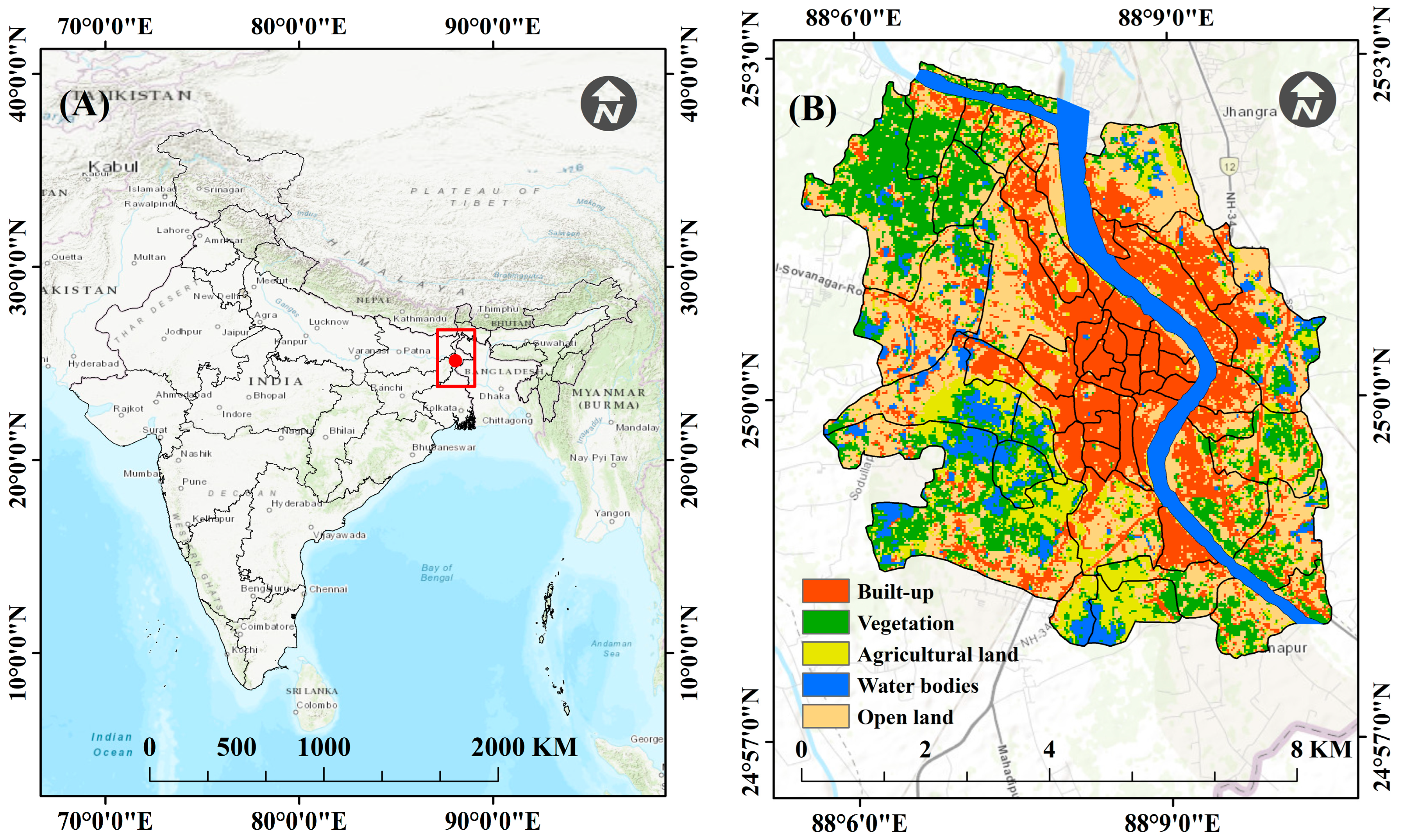
2.1. Study Area
2.2. Data Source
2.3. LST Extraction
2.4. LULC Mapping and Extraction of the IS, GS and BS
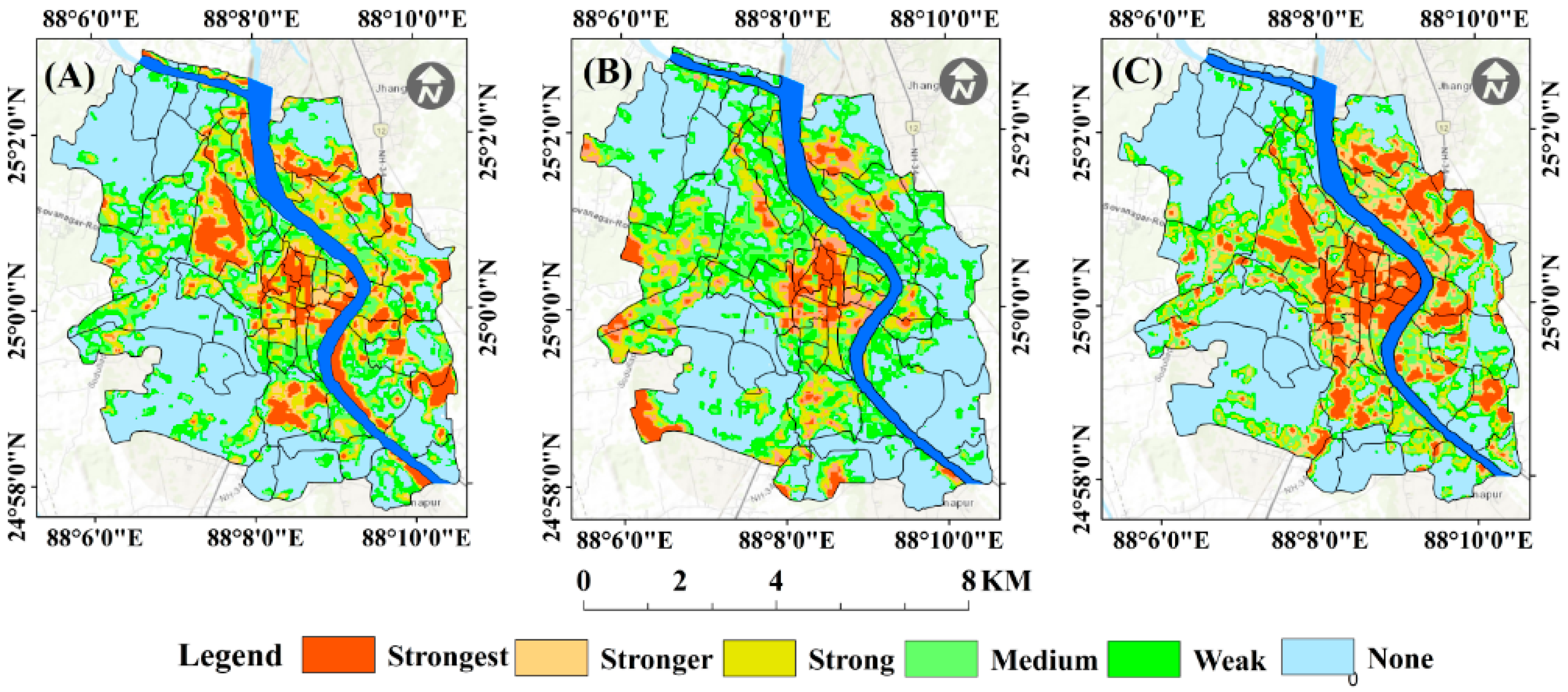
2.5. Delineation of UHI
2.6. Spatial and Statistical Analysis
2.6.1. Multi-Ring Approach
2.6.2. Spatial Metrics-Based Analysis
2.6.3. Validation
3. Results
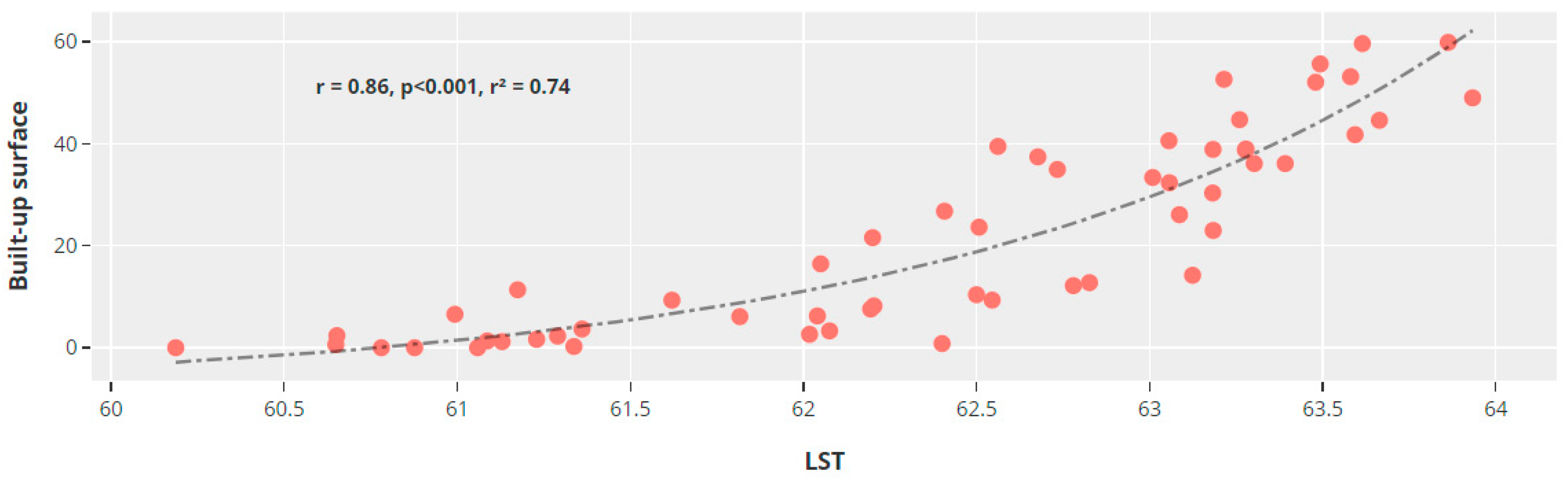
3.1. Validation
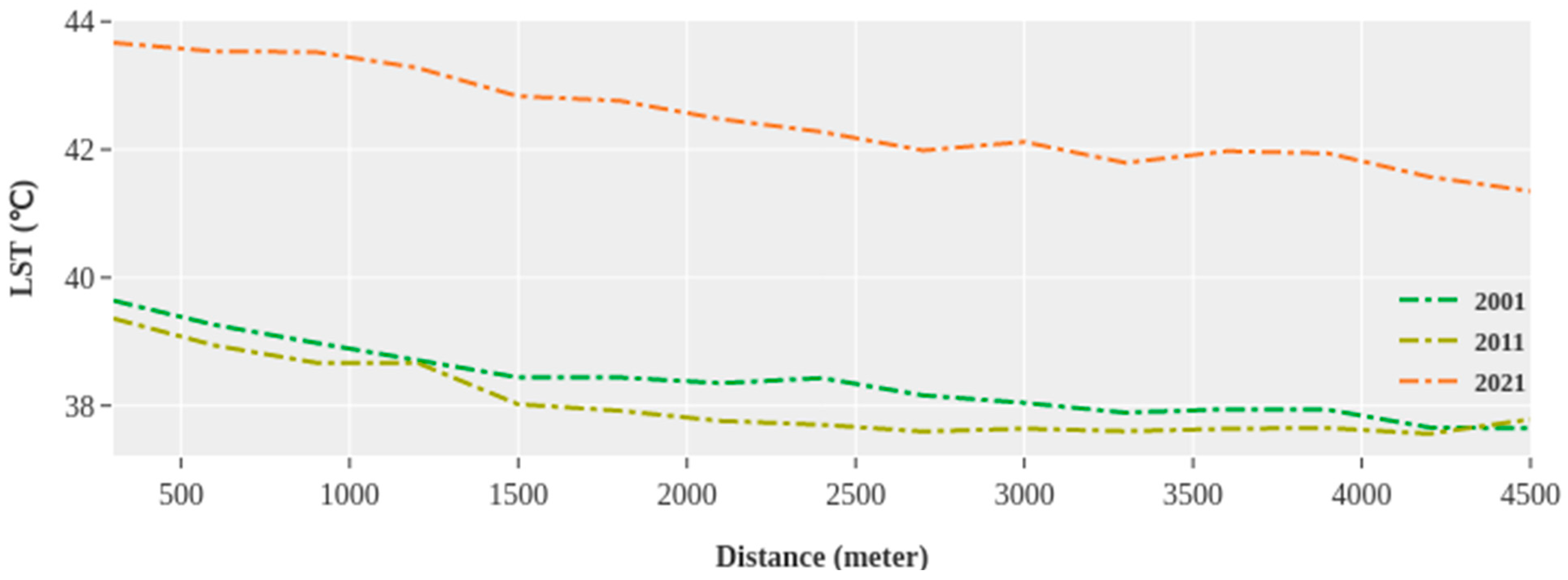
3.2. LST and UHI Pattern along URG
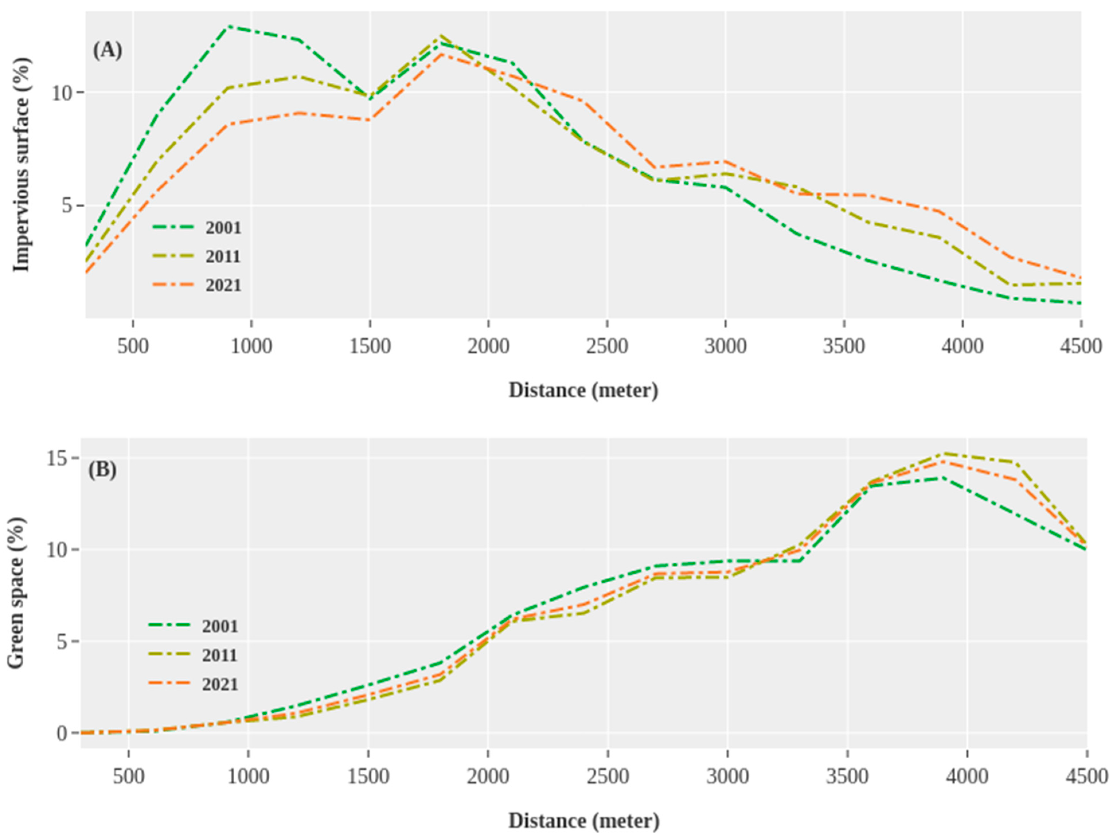
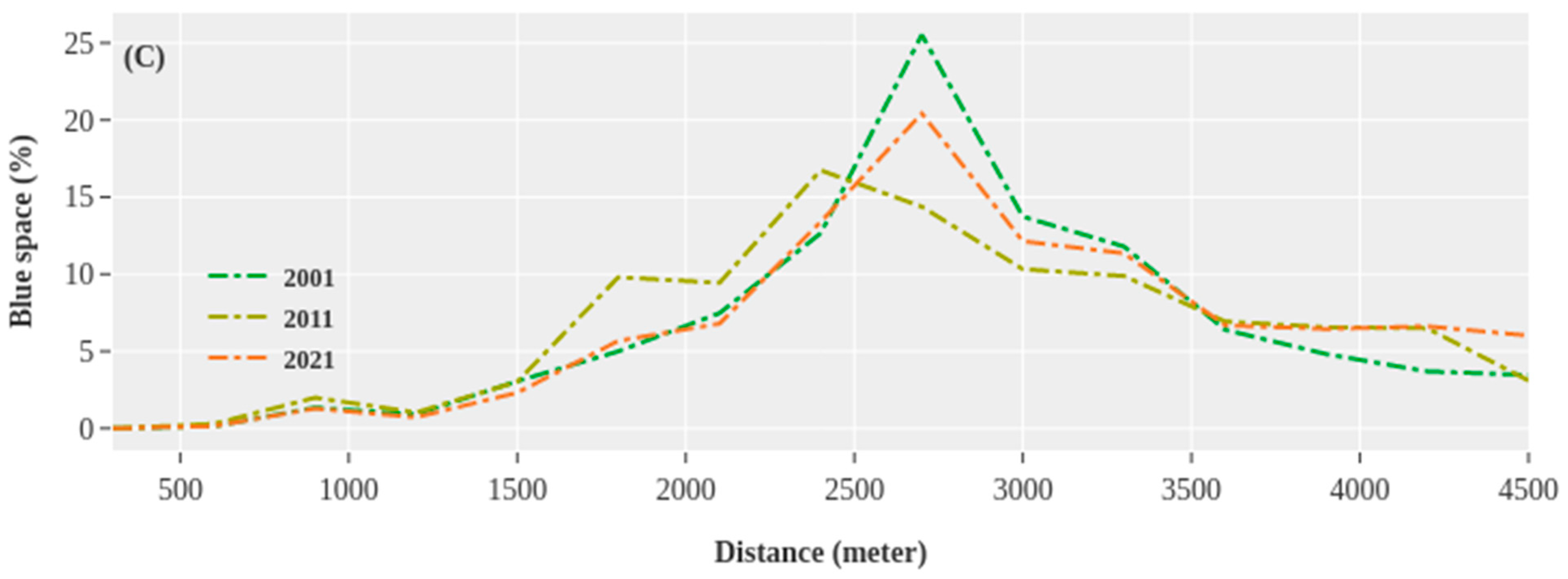
3.3. Changes of IS, GS, and BS along URG
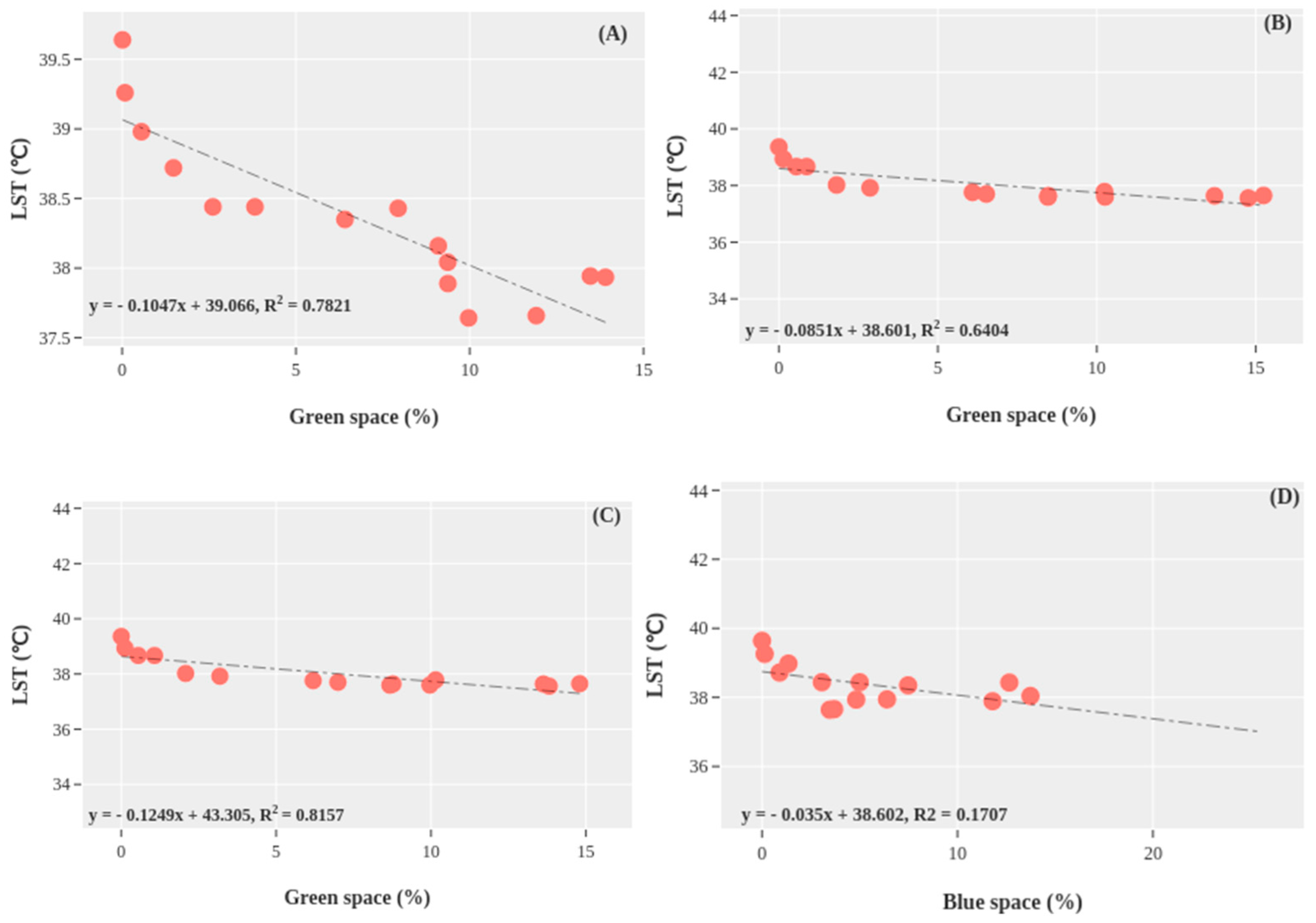
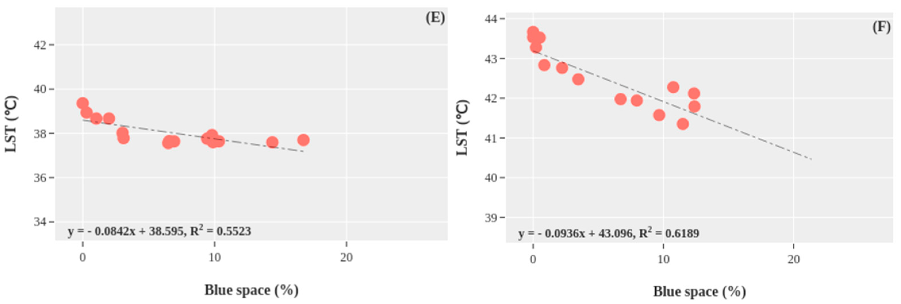
3.4. Impact of Landscape Composition and Configuration on the Thermal Environment
4. Discussion
4.1. Policy Implications
4.2. Limitations and Future Research Directions
5. Conclusions
Supplementary Materials
Author Contributions
Funding
Institutional Review Board Statement
Informed Consent Statement
Data Availability Statement
Conflicts of Interest
References
- Gallo, K.P.; Owen, T.W. Satellite-Based Adjustments for the Urban Heat Island Temperature Bias. J. Appl. Meteorol. 1999, 38, 806–813. [Google Scholar] [CrossRef]
- Guo, G.; Wu, Z.; Xiao, R.; Chen, Y.; Liu, X.; Zhang, X. Impacts of urban biophysical composition on land surface temperature in urban heat island clusters. Landsc. Urban Plan. 2015, 135, 1–10. [Google Scholar] [CrossRef]
- Lo, C.P.; Quattrochi, D.A.; Luvall, J.C. Application of high-resolution thermal infrared remote sensing and GIS to assess the urban heat island effect. Int. J. Remote Sens. 1997, 18, 287–304. [Google Scholar] [CrossRef]
- Singh, P.; Kikon, N.; Verma, P. Impact of land use change and urbanisation on urban heat island in Lucknow city, Central India. A remote sensing based estimate. Sustain. Cities Soc. 2017, 32, 100–114. [Google Scholar] [CrossRef]
- Du, H.; Ai, J.; Cai, Y.; Jiang, H.; Liu, P. Combined Effects of the Surface Urban Heat Island with Landscape Composition and Configuration Based on Remote Sensing: A Case Study of Shanghai, China. Sustainability 2019, 11, 2890. [Google Scholar] [CrossRef]
- Soydan, O. Effects of landscape composition and patterns on land surface temperature: Urban heat island case study for Nigde, Turkey. Urban Clim. 2020, 34, 100688. [Google Scholar] [CrossRef]
- Das, M.; Das, A. Exploring the pattern of outdoor thermal comfort (OTC) in a tropical planning region of eastern India during summer. Urban Clim. 2020, 34, 100708. [Google Scholar] [CrossRef]
- Saha, S.; Saha, A.; Das, M.; Saha, A.; Sarkar, R.; Das, A. Analyzing spatial relationship between land use/land cover (LULC) and land surface temperature (LST) of three urban agglomerations (UAs) of Eastern India. Remote Sens. Appl. Soc. Environ. 2021, 22, 100507. [Google Scholar] [CrossRef]
- Kedia, S.; Bhakare, S.P.; Dwivedi, A.K.; Islam, S.; Kaginalkar, A. Estimates of change in surface meteorology and urban heat island over northwest India: Impact of urbanisation. Urban Clim. 2021, 36, 100782. [Google Scholar] [CrossRef]
- Howard, L. The Climate of London: Deduced from Meteorological Observations Made in the Metropolis and at Various Places Around It. 1833, Volume 3. Available online: https://wellcomecollection.org/works/y73fcwsn (accessed on 29 December 2023).
- Voogt, J.A. Urban Heat Islands: Hotter Cities; America Institute of Biological Sciences: Herndon, VA, USA, 2004. [Google Scholar]
- Zhang, M.; Dong, S.; Cheng, H.; Li, F. Spatio-temporal evolution of urban thermal environment and its driving factors: Case study of Nanjing, China. PLoS ONE 2021, 16, e0246011. [Google Scholar] [CrossRef]
- Coseo, P.; Larsen, L. How factors of land use/land cover, building configuration, and adjacent heat sources and sinks explain Urban Heat Islands in Chicago. Landsc. Urban Plan. 2014, 125, 117–129. [Google Scholar] [CrossRef]
- Debbage, N.; Shepherd, J.M. The urban heat island effect and city contiguity. Comput. Environ. Urban Syst. 2015, 54, 181–194. [Google Scholar] [CrossRef]
- Lin, J.; Wei, K.; Guan, Z. Exploring the connection between morphological characteristic of built-up areas and surface heat islands based on MSPA. Urban Clim. 2024, 53, 101764. [Google Scholar] [CrossRef]
- Huang, Q.; Lu, Y. Urban heat island research from 1991 to 2015: A bibliometric analysis. Theor. Appl. Clim. 2018, 131, 1055–1067. [Google Scholar] [CrossRef]
- Deng, Y.; Wang, S.; Bai, X.; Tian, Y.; Wu, L.; Xiao, J.; Chen, F.; Qian, Q. Relationship among land surface temperature and LUCC, NDVI in typical karst area. Sci. Rep. 2018, 8, 64. [Google Scholar] [CrossRef] [PubMed]
- Guha, S.; Govil, H.; Dey, A.; Gill, N. Analytical study of land surface temperature with NDVI and NDBI using Landsat 8 OLI and TIRS data in Florence and Naples city, Italy. Eur. J. Remote Sens. 2018, 51, 667–678. [Google Scholar] [CrossRef]
- Maimaitiyiming, M.; Ghulam, A.; Tiyip, T.; Pla, F.; Latorre-Carmona, P.; Halik, Ü.; Sawut, M.; Caetano, M. Effects of green space spatial pattern on land surface temperature: Implications for sustainable urban planning and climate change adaptation. ISPRS J. Photogramm. Remote Sens. 2014, 89, 59–66. [Google Scholar] [CrossRef]
- Asgarian, A.; Amiri, B.J.; Sakieh, Y. Assessing the effect of green cover spatial patterns on urban land surface temperature using landscape metrics approach. Urban Ecosyst. 2015, 18, 209–222. [Google Scholar] [CrossRef]
- Sun, R.; Chen, L. Effects of green space dynamics on urban heat islands: Mitigation and diversification. Ecosyst. Serv. 2017, 23, 38–46. [Google Scholar] [CrossRef]
- Zhang, H.; Qi, Z.-F.; Ye, X.-Y.; Cai, Y.-B.; Ma, W.-C.; Chen, M.-N. Analysis of land use/land cover change, population shift, and their effects on spatiotemporal patterns of urban heat islands in metropolitan Shanghai, China. Appl. Geogr. 2013, 44, 121–133. [Google Scholar] [CrossRef]
- Bokaie, M.; Zarkesh, M.K.; Arasteh, P.D.; Hosseini, A. Assessment of Urban Heat Island based on the relationship between land surface temperature and Land Use/ Land Cover in Tehran. Sustain. Cities Soc. 2016, 23, 94–104. [Google Scholar] [CrossRef]
- Irfeey, A.M.M.; Chau, H.-W.; Sumaiya, M.M.F.; Wai, C.Y.; Muttil, N.; Jamei, E. Sustainable Mitigation Strategies for Urban Heat Island Effects in Urban Areas. Sustainability 2023, 15, 10767. [Google Scholar] [CrossRef]
- Shukla, A.; Jain, K. Critical analysis of rural-urban transitions and transformations in Lucknow city, India. Remote Sens. Appl. Soc. Environ. 2019, 13, 445–456. [Google Scholar] [CrossRef]
- Grover, A.; Singh, R.B. Analysis of urban heat island (UHI) in relation to normalised difference vegetation index (NDVI): A comparative study of Delhi and Mumbai. Environments 2015, 2, 125–138. [Google Scholar] [CrossRef]
- Dutta, I.; Das, A. Exploring the dynamics of urban sprawl using geo-spatial indices: A study of English Bazar Urban Agglomeration, West Bengal. Appl. Geomat. 2019, 11, 259–276. [Google Scholar] [CrossRef]
- Pal, S.; Ziaul, S. Detection of land use and land cover change and land surface temperature in English Bazar urban centre. Egypt. J. Remote Sens. Space Sci. 2017, 20, 125–145. [Google Scholar]
- Dutta, I.; Das, A. Exploring the Spatio-temporal pattern of regional heat island (RHI) in an urban agglomeration of secondary cities in Eastern India. Urban Clim. 2020, 34, 100679. [Google Scholar] [CrossRef]
- Ziaul, S.; Pal, S. Assessing outdoor thermal comfort of English Bazar Municipality and its surrounding, West Bengal, India. Adv. Space Res. 2019, 64, 567–580. [Google Scholar] [CrossRef]
- Kikon, N.; Singh, P.; Singh, S.K.; Vyas, A. Assessment of urban heat islands (UHI) of Noida City, India using multi-temporal satellite data. Sustain. Cities Soc. 2016, 22, 19–28. [Google Scholar] [CrossRef]
- Estoque, R.C.; Murayama, Y.; Myint, S.W. Effects of landscape composition and pattern on land surface temperature: An urban heat island study in the megacities of Southeast Asia. Sci. Total Environ. 2017, 577, 349–359. [Google Scholar] [CrossRef]
- Liu, G.; Zhang, Q.; Li, G.; Doronzo, D.M. Response of land cover types to land surface temperature derived from Landsat-5 TM in Nanjing Metropolitan Region, China. Environ. Earth Sci. 2016, 75, 1386. [Google Scholar] [CrossRef]
- McGarigal, K.; Cushman, S.A.; Neel, M.C.; Ene, E. FRAGSTATS: Spatial Pattern Analysis Program for Categorical Maps. Computer Software Program Produced by the Authors at the University of Massachusetts, Amherst. 2002. Available online: https://www.umass.edu/landeco/research/fragstats/fragstats.html (accessed on 29 December 2023).
- Boori, M.S.; Choudhary, K.; Paringer, R.; Kupriyanov, A. Spatiotemporal ecological vulnerability analysis with statistical correlation based on satellite remote sensing in Samara, Russia. J. Environ. Manag. 2021, 285, 112138. [Google Scholar] [CrossRef] [PubMed]
- Luo, J.; Zhuo, W.; Liu, S.; Xu, B. The Optimization of Carbon Emission Prediction in Low Carbon Energy Economy under Big Data. IEEE Access 2024. [Google Scholar] [CrossRef]
- Myint, S.W.; Brazel, A.; Okin, G.; Buyantuyev, A. Combined effects of impervious surface and vegetation cover on air temperature variations in a rapidly expanding desert city. GIScienceRemote Sens. 2010, 47, 301–320. [Google Scholar] [CrossRef]
- Sun, Q.; Wu, Z.; Tan, J. The relationship between land surface temperature and land use/land cover in Guangzhou, China. Environ. Earth Sci. 2012, 65, 1687–1694. [Google Scholar] [CrossRef]
- Song, J.; Du, S.; Feng, X.; Guo, L. The relationships between landscape compositions and land surface temperature: Quantifying their resolution sensitivity with spatial regression models. Landsc. Urban Plan. 2014, 123, 145–157. [Google Scholar] [CrossRef]
- Shang, K.; Xu, L.; Liu, X.; Yin, Z.; Liu, Z.; Li, X.; Yin, L.; Zheng, W. Study of Urban Heat Island Effect in Hangzhou Metropolitan Area Based on SW-TES Algorithm and Image Dichotomous Model. SAGE Open 2023, 13. [Google Scholar] [CrossRef]
- Li, X.; Zhou, W.; Ouyang, Z.; Xu, W.; Zheng, H. Spatial pattern of greenspace affects land surface temperature: Evidence from the heavily urbanised Beijing metropolitan area, China. Landsc. Ecol. 2012, 27, 887–898. [Google Scholar] [CrossRef]
- Zhou, W.; Huang, G.; Cadenasso, M.L. Does spatial configuration matter? Understanding the effects of land cover pattern on land surface temperature in urban landscapes. Landsc. Urban Plan. 2011, 102, 54–63. [Google Scholar] [CrossRef]
- Connors, J.P.; Galletti, C.S.; Chow, W.T.L. Landscape configuration and urban heat island effects: Assessing the relationship between landscape characteristics and land surface temperature in Phoenix, Arizona. Landsc. Ecol. 2013, 28, 271–283. [Google Scholar] [CrossRef]
- Das, M.; Das, A.; Momin, S. Quantifying the cooling effect of urban green space: A case from urban parks in a tropical mega metropolitan area (India). Sustain. Cities Soc. 2022, 87, 104062. [Google Scholar] [CrossRef]
- Wang, R.; Li, F.; Hu, D.; Li, B.L. Understanding eco-complexity: Social-Economic-Natural Complex Ecosystem approach. Ecol. Complex. 2011, 8, 15–29. [Google Scholar] [CrossRef]
- Shen, H.; Huang, L.; Zhang, L.; Wu, P.; Zeng, C. Long-term and fine-scale satellite monitoring of the urban heat island effect by the fusion of multi-temporal and multi-sensor remote sensed data: A 26-year case study of the city of Wuhan in China. Remote Sens. Environ. 2016, 172, 109–125. [Google Scholar] [CrossRef]
- Tian, P.; Li, J.; Cao, L.; Pu, R.; Wang, Z.; Zhang, H.; Chen, H.; Gong, H. Assessing spatiotemporal characteristics of urban heat islands from the perspective of an urban expansion and green infrastructure. Sustain. Cities Soc. 2021, 74, 103208. [Google Scholar] [CrossRef]
- Yang, H.; Zhang, X.; Li, Z.; Cui, J. Region-Level Traffic Prediction Based on Temporal Multi-Spatial Dependence Graph Convolutional Network from GPS Data. Remote Sens. 2022, 14, 303. [Google Scholar] [CrossRef]
- Zhou, X.; Chen, H. Impact of urbanisation-related land use land cover changes and urban morphology changes on the urban heat island phenomenon. Sci. Total Environ. 2018, 635, 1467–1476. [Google Scholar] [CrossRef]
- Das, M.; Das, A. Dynamics of Urbanization and its impact on Urban Ecosystem Services (UESs): A study of a medium size town of West Bengal, Eastern India. J. Urban Manag. 2019, 8, 420–434. [Google Scholar] [CrossRef]
- Das, M.; Das, A.; Pereira, P.; Mandal, A. Exploring the spatio-temporal dynamics of ecosystem health: A study on a rapidly urbanising metropolitan area of Lower Gangetic Plain, India. Ecol. Indic. 2021, 125, 107584. [Google Scholar] [CrossRef]
- Qin, Y. A review on the development of cool pavements to mitigate urban heat island effect. Renew. Sustain. Energy Rev. 2015, 52, 445–459. [Google Scholar] [CrossRef]
- Lu, S.; Zhu, G.; Meng, G.; Lin, X.; Liu, Y.; Qiu, D.; Xu, Y.; Wang, Q.; Chen, L.; Li, R.; et al. Influence of atmospheric circulation on the stable isotope of precipitation in the monsoon margin region. Atmos. Res. 2024, 298, 107131. [Google Scholar] [CrossRef]
- Sharma, A.; Conry, P.; Fernando, H.J.S.; Hamlet, A.F.; Hellmann, J.J.; Chen, F. Green and cool roofs to mitigate urban heat island effects in the Chicago metropolitan area: Evaluation with a regional climate model. Environ. Res. Lett. 2016, 11, 064004. [Google Scholar] [CrossRef]
- Saaroni, H.; Amorim, J.H.; Hiemstra, J.A.; Pearlmutter, D. Urban Green Infrastructure as a tool for urban heat mitigation: Survey of research methodologies and findings across different climatic regions. Urban Clim. 2018, 24, 94–110. [Google Scholar] [CrossRef]
- Farhadi, H.; Faizi, M.; Sanaieian, H. Mitigating the urban heat island in a residential area in Tehran: Investigating the role of vegetation, materials, and orientation of buildings. Sustain. Cities Soc. 2019, 46, 101448. [Google Scholar] [CrossRef]
- Aram, F.; Solgi, E.; García, E.H.; Mosavi, A.; Várkonyi-Kóczy, A.R. The Cooling Effect of Large-Scale Urban Parks on Surrounding Area Thermal Comfort. Energies 2019, 12, 3904. [Google Scholar] [CrossRef]


| Basic Information | |
|---|---|
| Name | English Bazar Urban Agglomeration (EBUA) |
| City type | Class I city (sixth largest urban agglomerations in West Bengal) |
| Local bodies | (i) Municipalities (English Bazar and Old Malda), (ii) Census towns, (iii) Mouzas (16 from English Bazar block and 11 from Old Malda block) |
| Urban bodies | 2 municipalities, |
| Area (km2) | 5465.43 ha [28] |
| Geographical location | Diara region in lower Gangetic plain |
| Demographic profile | |
| Total population | 0.63 million |
| Population density (person/km2) | 13,861 |
| Decadal growth (%) | 21.5 |
| Climatic features | |
| Climate type | Sub-tropical monsoon |
| Season | (i) Monsoon–June to mid of October; (ii) Post-monsoon–mid of October to mid of December; (iii) Winter–January to February, and (iv) Pre-monsoon (Summer)–March to May |
| Temperature (°C) in winter | About 10 |
| Temperature (°C) in summer | About 35 |
| Precipitation (mm) | 1444 |
| Year | Specification of Date | Image ID | Resolution (Meter) | Sensor |
|---|---|---|---|---|
| 2001 | 25 April | LT05_L2SP_139043_20010425_20200906_02_T1 | 30 | Thematic mapper (TM) |
| 2011 | 4 April | LT05_L2SP_139043_20110421_20200822_02_T1 | 30 | Thematic mapper (TM) |
| 2021 | 15 March | LC08_L2SP_139043_20210315_20210328_02_T1 | 30 (100 m for thermal band) | Operational Landsat imager |
| Spatial Metrics | Acronym | Description |
|---|---|---|
| Mean patch area | AREA_MN | It is used to measure the area or size of the patch |
| It is the sum of all patches of the corresponding path types. It is calculated from the patch metrics values divided by the number of patches. | ||
| The equation of AREA_MN = | ||
| Mean patch index | SHAPE_MN | It is one of the simplest measures of shape complexity |
| It is calculated from the patch perimeter and square root of the patch areas, adjusted by a constant to adjust a square standard, and divided by the number of patches. | ||
| The equation of SHAPE_MN = . | ||
| Aggregation index | AI | It is the number of like adjacencies divided by the maximum possible number of the adjacencies (corresponding class). |
| The equation of AI = | ||
| The value of AI “0” means totally disaggregated (no adjacencies), and 100 means patch type is totally aggregated, indicating a single patch. |
| Landscapes | Statistics | AREA_MN (ha) | SHAPE_MN (ha) | AI (%) |
|---|---|---|---|---|
| IS | Mean | 22.51 | 1.86 | 73.22 |
| SD | 40.12 | 1.23 | 17.64 | |
| Skewness | 2.09 | 1.61 | −0.17 | |
| Kurtosis | 3.91 | 2.36 | −1.26 | |
| Correlation with mean LST | r | 0.703 ** | 0.217 | 0.960 ** |
| Sig (2-tailed) | 0.003 | 0.437 | 0.000 | |
| GS | Mean | 0.77 | 1.21 | 43.19 |
| SD | 0.55 | 0.40 | 28.93 | |
| Skewness | 0.58 | −1.64 | −0.78 | |
| Kurtosis | 0.37 | 7.00 | −1.19 | |
| Correlation with mean LST | r | −0.896 ** | −0.363 | −0.952 ** |
| Sig (2-tailed) | 0.000 | 0.1784 | 0.00 | |
| BS | Mean | 0.64 | 1.12 | 49.02 |
| SD | 0.47 | 0.34 | 24.15 | |
| Skewness | 1.15 | −1.99 | −1.12 | |
| Kurtosis | 1.67 | 6.89 | 0.02 | |
| Correlation with mean LST | r | −0.800 ** | −0.686 ** | −0.722 ** |
| Sig (2-tailed) | 0.000 | 0.005 | 0.002 |
Disclaimer/Publisher’s Note: The statements, opinions and data contained in all publications are solely those of the individual author(s) and contributor(s) and not of MDPI and/or the editor(s). MDPI and/or the editor(s) disclaim responsibility for any injury to people or property resulting from any ideas, methods, instructions or products referred to in the content. |
© 2024 by the authors. Licensee MDPI, Basel, Switzerland. This article is an open access article distributed under the terms and conditions of the Creative Commons Attribution (CC BY) license (https://creativecommons.org/licenses/by/4.0/).
Share and Cite
Das, A.; Saha, P.; Dasgupta, R.; Inacio, M.; Das, M.; Pereira, P. How Do the Dynamics of Urbanization Affect the Thermal Environment? A Case from an Urban Agglomeration in Lower Gangetic Plain (India). Sustainability 2024, 16, 1147. https://doi.org/10.3390/su16031147
Das A, Saha P, Dasgupta R, Inacio M, Das M, Pereira P. How Do the Dynamics of Urbanization Affect the Thermal Environment? A Case from an Urban Agglomeration in Lower Gangetic Plain (India). Sustainability. 2024; 16(3):1147. https://doi.org/10.3390/su16031147
Chicago/Turabian StyleDas, Arijit, Priyakshi Saha, Rajarshi Dasgupta, Miguel Inacio, Manob Das, and Paulo Pereira. 2024. "How Do the Dynamics of Urbanization Affect the Thermal Environment? A Case from an Urban Agglomeration in Lower Gangetic Plain (India)" Sustainability 16, no. 3: 1147. https://doi.org/10.3390/su16031147
APA StyleDas, A., Saha, P., Dasgupta, R., Inacio, M., Das, M., & Pereira, P. (2024). How Do the Dynamics of Urbanization Affect the Thermal Environment? A Case from an Urban Agglomeration in Lower Gangetic Plain (India). Sustainability, 16(3), 1147. https://doi.org/10.3390/su16031147