Assessment of a Temperature-Based Artificial Neural Network Designed for Global Solar Radiation Estimation in Regions with Sparse Experimental Data

Abstract

The aim is to evaluate a model of monthly mean global solar radiation based on a simple ANN that uses geographic and temperature data as input variables and is designed for estimations in regions with few radiometric stations. Using data from 414 Spanish stations, the performance of the model is evaluated when both the number and the percentage of data collected for training the network are significantly modified while maintaining the clustering algorithms. The statistical indicators obtained show a compromise between achieving a lower mean error for all stations and limiting the maximum error at each station. In the worst case, the average error is less than 10% for all stations, and the maximum local error only exceeds 20% in less than 2% of the estimates. The least accurate predictions seem to be related to climate types where the clearness index tends to be higher in winter than in summer, which is the case in some locations on the northern Spanish coast. The results are consistent with estimates obtained for 16 non-Spanish stations, selected within the same input data range, suggesting that the variation of the clearness index over the year could be an important factor for local climate characterization.

1. Introduction

Renewable energy sources, mainly wind or solar, are currently considered essential for sustainable access to humanity’s basic resources, i.e., water, food, and energy [1], and for climate change mitigation, which is critical to protect humans, wildlife, and ecosystems [2]. Solar energy serves as a cornerstone for policymakers, engineers, and researchers [3] and is also discussed in educational projects for sustainability [4]. Thus, reliable data on solar resources are therefore needed to support the sustainable growth and impact of solar installations [5,6].

Solar resource assessment requires relatively expensive direct measurement equipment operating at qualified meteorological stations and providing long data sets to facilitate the validation of solar radiation models. Since radiometric stations are relatively scarce, especially in less developed countries [7,8], it is interesting to develop models that allow indirect estimation of global solar radiation (GSR) from abundantly recorded meteorological variables such as temperature.

Numerous GSR models have been developed over decades [9,10,11]. The accuracy of the estimates depends not only on the methodology and the number and type of influential variables considered in the model but also on the quality and the spatial and temporal distribution of the used data [12,13]. Models have even been proposed that use non-meteorological input variables, such as declination [14] or latitude [15], penalizing accuracy at the expense of simplicity. In general, it can be said that most GSR models are acceptable for the localities or regions where they were validated but less accurate when extended to other areas [16].

There is a trade-off between the accuracy of a model, its complexity, and its generality, i.e., its adaptability to large regions. Accuracy at the local scale can be increased using a higher number of variables, but a simple model may have advantages for predictions over large regions due to its higher number of degrees of freedom [17]. In addition, generality can be facilitated using dimensionless variables and complete functional relationships, i.e., dimensionally homogeneous equations. Otherwise, the parameters or coefficients of the functional relationships necessarily depend on variables that are not explicit in the model [11]. This observation has been little emphasized so far and is applicable to both regression-based and artificial intelligence-based models.

The most widely used models for estimating GSR consist of expressions of the clearness index as a function of the relative sunshine duration, so they are dimensionally homogeneous equations with various mathematical forms. Most equations use site-dependent parameters, but some of them are intended to be valid worldwide. Around 90% of the variability in data recorded at 59 European stations has been explained using relative sunshine hours, elevation, and the monthly index as input variables [18], but data on sunshine duration are not generally available. Looking for a temperature-based approach and as an evolution of the classical model of Hargreaves and Samani [19], a model of the monthly average of the atmospheric clearness index has been previously introduced [20], using the square root of $∆T/T_{\mathrm{m}\mathrm{i}\mathrm{n}}$ as the only meteorological variable, where $∆T$ is the difference between the monthly average of daily maximum temperature, $T_{\mathrm{m}\mathrm{a}\mathrm{x}}$ (in K), and the monthly average of daily minimum temperature, $T_{\mathrm{m}\mathrm{i}\mathrm{n}}$ (in K), and assuming that the proportionality coefficient depends on the ratio $z/L$ between the elevation $z$ (in m) and the distance to the sea $L$ (in km). This simple and dimensionally homogeneous model has been evaluated with acceptable results in localities of the northern Spanish coast [11,12,13,17,20] and two large areas of central and southern Spain, with very different climatology and latitude. The comparison with other temperature-based models in each of the three zones showed both the advantages of this model for obtaining general equations applicable in each zone and the influence of latitude on the geographical variability of the model coefficients [12].

To analyze the influence of latitude, mathematical methodology, and possible seasonal effects, a model based on a simple ANN was recently developed to estimate the monthly clearness index for the set of 105 stations located in the three areas of peninsular Spain previously studied. Using $∆T/T_{\mathrm{m}\mathrm{i}\mathrm{n}}$, $z/L$, the latitude and a monthly index as input variables. This approach allowed the improvement of the accuracy of previous models for both statistical indicators averaged for the set of stations and local deviations [13].

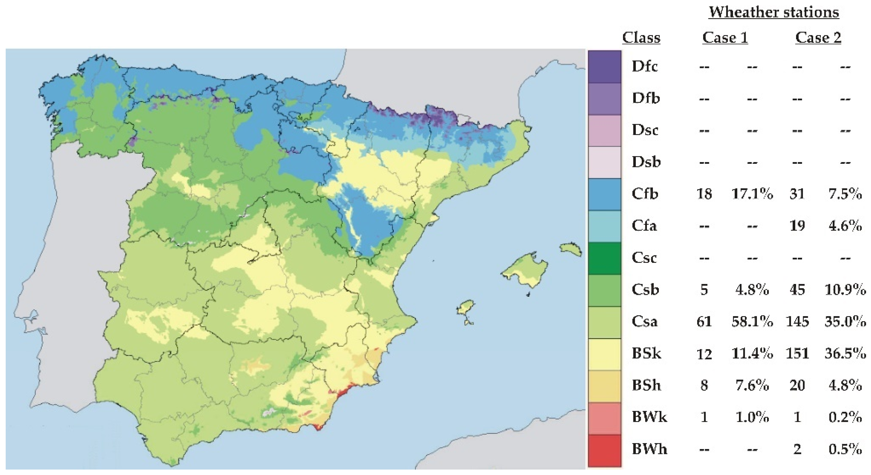
The varied geography and orography of Spain have been considered in many studies to characterize the solar resource, using different methods and data from a smaller number of on-ground stations than in the present article [21,22,23]. Access to the network of the Spanish Ministry of Agriculture, Fisheries and Food’s Agroclimatic Information System for Irrigation (SIAR) has facilitated for this paper the evaluation of the model using data from a total of 414 on-ground stations.

The main objective of the paper is to answer the following three research questions:

(a)

Is the robustness of the model, based on a simple ANN using the most commonly available input variables, acceptable when the percentage of data collected for network testing is significantly increased while maintaining the clustering algorithms?

(b)

What would the result be if a similar percentage of data were used for training and testing?

(c)

Does the procedure allow the detection of any climatic characteristics to improve the estimates without adding input variables?

To investigate the first question, the scenario described in the previous paper is considered to be a starting point (Case 0), using 53 stations for ANN training and 52 for testing. Case 1 refers to the ANN trained with the same 53 stations as in Case 0, but using for validation the remaining 361 stations available after adding the SIAR database.

In the analysis of the second question, Case 2 refers to the behavior of the ANN re-trained with 206 stations and validated with the remaining 208 stations.

Finally, to address the third question and as a preliminary step for more comprehensive future work on the extension of the procedure to other countries, the ANN results for the Spanish stations are complemented with ANN results for 16 stations included in the Meteonorm database [24].

Regarding the article’s structure, the Materials and Methods section contains descriptions of the physical and mathematical foundations of the model, the data, and the analysis procedure employed. In the Results section, it is considered an interesting contribution to show the statistical distribution of data in the cases analyzed, as well as the use of relative errors, both local and averaged over the total data set, as statistical indicators of the accuracy. After being previously described, the results are interpreted in the Discussion section in response to the research questions posed as objectives.

From a practical point of view, it is considered that the model procedure may be of interest for low-cost solar resource assessments at the microclimate scale, using data from secondary thermometric networks, terrain elevation maps, and GIS techniques once the model is validated on a wide range of input variables.

From an academic point of view, the article is an additional contribution to the scarce general GSR models, where the rare use of dimensionless variables is surprising despite being more orthodox from a physics point of view and more advantageous from a computational perspective.

2. Materials and Methods

2.1. Model Fundamentals

Any physical model is based on a functional relationship between quantities, even if it has an unknown mathematical form. In this article, the monthly average global solar irradiation on horizontal surface $H$ is assumed to be dependent on the monthly average extraterrestrial irradiation $H_0$, on the already defined temperature amplitude $∆T$, on the monthly average of daily minimum temperature $T_{\mathrm{m}\mathrm{i}\mathrm{n}}$, on the elevation $z$, on the distance to the sea $L$, on the latitude $\varphi$, and on a monthly index $d$, i.e.,:

$$H=f\left(H_0,∆T,T_{\mathrm{m}\mathrm{i}\mathrm{n}},z,L,\varphi ,d\right).$$

(1)

Parametric model equations are called incomplete when they cannot be converted into dimensionally homogeneous expressions, i.e., they cannot be rewritten by means of dimensionless groups formed by products of powers of the original ordinary quantities. Therefore, dimensional homogeneity analysis makes it possible to detect the absence of influential variables in a model. Using this type of reasoning, the original Hargreaves and Samani model was previously converted into a complete equation by adding $T_{\mathrm{m}\mathrm{i}\mathrm{n}}$, $z$ and $L$ as variables influencing the clearness index [20]. The procedure is also applicable to transfer functions used in ANN-based models, which satisfy relationships of the following type:

$$y_j=f\left({\sum }_{i=1}^n{w}_{ij}{x}_i+k_j\right),$$

(2)

where $y_j$, $x_i$, $w_{ij}$, and $k_j$ denote components of the output vector, the input vector, the connection weight matrix, and the independent term, respectively [25]. Buckingham’s Pi theorem provides an operational method to obtain the influencing non-dimensional groups, whose number is generally smaller than the original number of ordinary variables. If the application of the theorem does not lead to a solution, it is undoubtedly because the starting relationship is incomplete. In the case of Equation (1), the application of the theorem leads to the following equivalent expression, which justifies the selection of model input variables to estimate the atmospheric clearness index:

$${\displaystyle \frac{H}{H_0}}=f\left({\displaystyle \frac{∆T}{T_{\mathrm{m}\mathrm{i}\mathrm{n}}}},{\displaystyle \frac{z}{L}},\varphi ,d\right).$$

(3)

2.2. Data Bases

Table S1 in Supplementary Data shows the geographical and topographical data, as well as the Köppen–Geiger climate classification of the 414 radiometric stations used in this article, either for training or validation purposes. Stations No.1 to 105 are those used in previous works [12,13,17], operated by the Spanish State Meteorological Agency, Spanish Ministry of Environmental Issues, Environmental Climatology Information Network of the Andalusian Regional Government, Service of Environmental Information of the Principality of Asturias, and City Council of Gijón. Stations No.106 to 414 are the ones introduced in this paper, operated by the Spanish Ministry of Agriculture, Fisheries and Food. Figure 1 shows the distribution of the 414 stations, according to the Köppen–Geiger climate classification [26]. The variety of geographical, topographical, and climatic characteristics considered is representative of practically the whole of peninsular Spain, while stations No.369 to 376 facilitate the extension of the study to the Balearic Islands. At almost all stations, records averaged over a minimum of 14 years of the last two decades are used.

Table S2 in Supplementary Data shows experimental values of monthly averages of maximum and minimum daily temperatures and daily global solar irradiation on horizontal surfaces, as well as calculated values of monthly averages of daily extraterrestrial irradiation, totaling 4968 data for each variable.

Data compiled from the Meteonorm database [24] for stations in other countries are labeled as stations No.415 to 430 in Tables S3 and S4 of Supplementary Data.

Figure 2 shows the data distributions of the input variables used in Case 0, which fall within the following ranges:

$$0.0122\le ∆T/T_{\mathrm{m}\mathrm{i}\mathrm{n}}\le 0.0756$$

$$36.29°\le \varphi \le 43.58°$$

$$0.22\le z/L\le 376.65$$

Figure 3 shows the data distributions of the input variables used in Cases 1 and 2, which fall within the following ranges:

$$0.0122\le ∆T/T_{\mathrm{m}\mathrm{i}\mathrm{n}}\le 0.0787$$

$$36.29°\le \varphi \le 43.58°$$

$$0.00\le z/L\le 377.77$$

2.3. Hierarchical Clustering

Following the procedure of previous work [27], the available stations were classified into representative clusters by means of a bottom-up hierarchical clustering algorithm based on Euclidian distance and median merging criteria. Hierarchical clustering has been used in many areas, such as the analysis of residential energy consumption in Spain [28]. It was also recently recommended to perform solar radiation clustering, which led to the closest results to the Köppen–Geiger classification based on comparisons of four methods using data from 76 Spanish stations, two of which are located in northern coastal provinces [29].

Since some variables have values of some orders of magnitude higher than others, to avoid over-representation of these variables in the clustering procedure, the data have been previously normalized with the following equations:

$${\left({\displaystyle \frac{∆T}{T_{\mathrm{m}\mathrm{i}\mathrm{n}}}}\right)}_i^{*}={\displaystyle \frac{{\left(\frac{∆T}{T_{\mathrm{m}\mathrm{i}\mathrm{n}}}\right)}_i-\underset{j=1\dots n}{\min }\left\{{\left(\frac{∆T}{T_{\mathrm{m}\mathrm{i}\mathrm{n}}}\right)}_j\right\}}{\underset{j=1\dots n}{\max }\left\{{\left(\frac{∆T}{T_{\mathrm{m}\mathrm{i}\mathrm{n}}}\right)}_j\right\}-\underset{j=1\dots n}{\min }\left\{{\left(\frac{∆T}{T_{\mathrm{m}\mathrm{i}\mathrm{n}}}\right)}_j\right\}}}$$

(4)

$${\left({\displaystyle \frac{z}{L}}\right)}_i^{*}={\displaystyle \frac{{\left(\frac{z}{L}\right)}_i-\underset{j=1\dots n}{\mathit{min}}\left\{{\left(\frac{z}{L}\right)}_j\right\}}{\underset{j=1\dots n}{\mathit{max}}\left\{{\left(\frac{z}{L}\right)}_j\right\}-\underset{j=1\dots n}{\mathit{min}}\left\{{\left(\frac{z}{L}\right)}_j\right\}}}$$

(5)

$${\varphi }_i^{*}={\displaystyle \frac{{\varphi }_i-\underset{j=1\dots n}{\mathit{min}}\left\{{\varphi }_j\right\}}{\underset{j=1\dots n}{\mathit{max}}\left\{{\varphi }_j\right\}-\underset{j=1\dots n}{\mathit{min}}\left\{{\varphi }_j\right\}}}$$

(6)

where $n$ is the number of stations, ${\left(∆T/T_{\mathrm{m}\mathrm{i}\mathrm{n}}\right)}_i$ is the annual average value for i-th station, calculated from the monthly average values ${\left(∆T/T_{\mathrm{m}\mathrm{i}\mathrm{n}}\right)}_i^m$ using the following equation:

$${\left({\displaystyle \frac{∆T}{T_{\mathrm{m}\mathrm{i}\mathrm{n}}}}\right)}_i={\displaystyle \frac{1}{12}}\sum _{m=1}^{12}{\left({\displaystyle \frac{∆T}{T_{\mathrm{m}\mathrm{i}\mathrm{n}}}}\right)}_i^m,$$

(7)

2.4. ANN Characteristics

From a biological standpoint, a neuron can be defined as a living element placed inside a network of similar organisms, which provides it with a series of inputs. Then, an output is given [30] based on internal calculations. Following the structure of an ANN, its elements can be sorted into different groups. The neurons of the input layer act as the entrance of the numerical values of the variables $x_1,\dots ,x_n$ used to obtain the exit variables $a_1,\dots ,a_k$ of the network. It also carries information to the elements within the hidden layers. In this sense, the number of hidden layers can be as high as required to meet the required behavior. It is worth noting that its complexity and, thus, its optimization will be increased with this number. The output of each neuron is computed using Equation (2). The variable $y_j$ represents the output of the j-th element, which is the result of the activation function $f$, given a linear combination of the outputs of the previous layer. Thus, $x_i$ is the input of the i-th neuron from the previous layer; $w_{ij}$ is the gain factor of each excitation from the previous layer, and $k_j$ denotes an independent term. The function $f$ is introduced to produce a non-linearity in the system. According to the literature, it could be, among different options, an arctangent, a sigmoid, or a ramp function [25].

The complexity of an ANN makes it unfeasible to find an analytic solution directly, given the number of variables involved. Therefore, a training process is required. In this sense, a cost function is defined to be used in a convergence algorithm. It is aimed to obtain for each neuron the weights and biases in Equation (2) that optimize this function. The application of Buckingham’s theorem to the functional relation underlying the ANN simplifies the structure of the ANN, providing computational advantages due to the smaller number of variables and weights. The general results are evaluated by comparing the network output with the objective values by means of statistical indicators.

Multiple algorithms can be used in the process, with each single one of them having a different variation. A review of the great variation of them can be found in [31]. In general, one should not be chosen over the others, as there is a plethora of variations for each single one of them. Depending on the structure of the ANN, some may obtain the solution faster or be more suitable for more complex networks; however, the study of the best optimization process is outside the scope of this paper. As already mentioned, the behavior of the ANN previously introduced and applied to data recorded at 105 stations in three large areas of Spain (Case 0) will be evaluated in the following sections with a different set of data. The network structure consists of 3 hidden layers, connected by 15 neurons in each one. In this manuscript, a modification of the gradient algorithm is used to find the final parameters of the ANN during the training process. In this case, a value of any of the parameters of the network ($k_j$ or $w_{ij}$) is chosen randomly and then modified by adding or subtracting a certain quantity. If the cost function is improved with the change, this is kept. Then, the process is repeated until the cost function reaches a certain threshold.

2.5. Statistical Indicators

Several methods have been proposed to assess the fit between experimental observations and model estimates, but none of them is free of limitations [32]. Since percentage results are easier to interpret, this paper will make comparisons between models using dimensionless statistical indicators, namely the relative root-mean-square error (RRMSE), the relative mean bias error (RMBE), and the coefficient of determination $\left(R^2\right)$. To facilitate comparisons with the results of other authors, the Nash–Sutcliffe model efficiency coefficient (NSE), the normalized mean square error (NRMSE), and mean bias error (NMBE) have also been calculated, in both cases using the mean value of the experimental data as the reference for the normalization. In addition, comparisons based on the centered pattern RMS difference provide a concise summary statistic in terms of their correlation, their root-mean-square difference, and the ratio of their variances, as can be deduced from the following relationship:

$$E_n^{\prime }=\sqrt{1+{\sigma }_{sn}^2-2{\sigma }_{sn}R}$$

(8)

where ${\sigma }_{sn}$ is the standard deviation of the clearness index estimates, normalized by the standard deviation of the experimental data.

Regarding the performance at the local scale, the assessments will be made in terms of monthly relative errors and their probabilistic distribution.

3. Results

3.1. Number of Clusters and Selection of Training and Testing Data

Among the various criteria in the literature for determining the number of clusters, the one proposed by Kaushik has been adopted [27]. This procedure is based on the construction of the dendrogram and recommends that the number of clusters is the number of vertical lines cut in the dendrogram by a horizontal line that can traverse the maximum distance vertically without intersecting a cluster.

From the dendrogram shown in Figure 4, it is deduced that 4 clusters are obtained for the 414 stations considered in Cases 1 and 2. The stations included in each cluster are specified in

Table 1. Distribution of stations in each cluster.

Cluster No.1	Cluster No.2	Cluster No.3	Cluster No.4
91, 92, 103	85, 86, 87, 88, 89, 90, 93, 94, 95, 97, 98, 99, 100, 367	4, 7, 9, 10, 11, 13, 15, 17, 18, 20, 23, 24, 44, 60, 389, 399	Rest of stations

, and the distributions of stations and clusters in the normalized space are shown in Figure 5. Cluster No.1 includes only 3 stations, which are very close to the Cantabrian coastline and have a Cfb-type climate. The 14 stations included in Cluster No.2 are also located on the north coast, 11 of which have a Cfb climate, and the remaining ones have a Csb climate. Cluster No.3 includes 7 stations with climate type Csa, 5 stations type BSh, 4 stations type BSk, and 2 stations type BWh, some of them with relatively high $z/L$ values, especially station No.24, whose $z/L$ value is only surpassed by the stations of Cluster No.1. Cluster No.4 is much bigger than others are, as it includes 381 stations, which represent 92% of the stations, and has a greater climatic variety.

For Case 2, approximately half of the stations in each cluster were randomly selected for training or validation purposes, amounting to a total of 206 training stations and 208 testing stations.

Table 2. Distribution of training stations in each cluster for Case 2.

Cluster No.1	Cluster No.2	Cluster No.3	Cluster No.4
91, 103	86, 88, 90, 93, 95, 97, 99	4, 10, 18, 20, 24, 44, 60, 399	2, 6, 8, 12, 14, 16, 22, 26–42 (even), 46–58 (even), 62–84 (even), 96, 101, 105–365 (odd), 369–387 (odd), 391–397 (odd), 401–413 (odd)

lists the distribution of the training stations in the clusters. It can be observed that 189 of the training stations belong to Cluster No.4, representing 92% of the training stations.

3.2. ANN Performance for the Set of 414 Spanish Stations

Figure 6 compares the experimental values and the neural network estimates for Case 1, using symbols to differentiate the stations used for training and testing in Case 0 and the remaining stations added from the SIAR network. Figure 7 compares the results obtained after having re-trained the neural network for Case 2.

Table 3. Statistical indicators for Cases 1 and 2.

	RRMSE (%)	RMBE (%)	NRMSE (%)	NMBE (%)	NSE	R2	${\mathit{\sigma }}_{\mathit{s}\mathit{n}}$	${\mathit{E}}_{\mathit{n}}^{\prime }$ (%)
Case 1	9.28	−5.41	9.44	−0.68	0.4591	0.6762	0.9638	58.64
Case 2	6.89	−0.30	6.33	−0.67	0.7570	0.7628	0.9282	49.01

allows the comparison of the statistical results in both cases. The RRMSE value obtained in Case 2 for the training and testing stations is very similar, in the order of 6.9%, which indicates that the stations chosen for training represent acceptably the testing stations. Figure 8 allows a comparison between the two cases by means of a Taylor diagram, which is based on Equation (8) [33].

4. Discussion

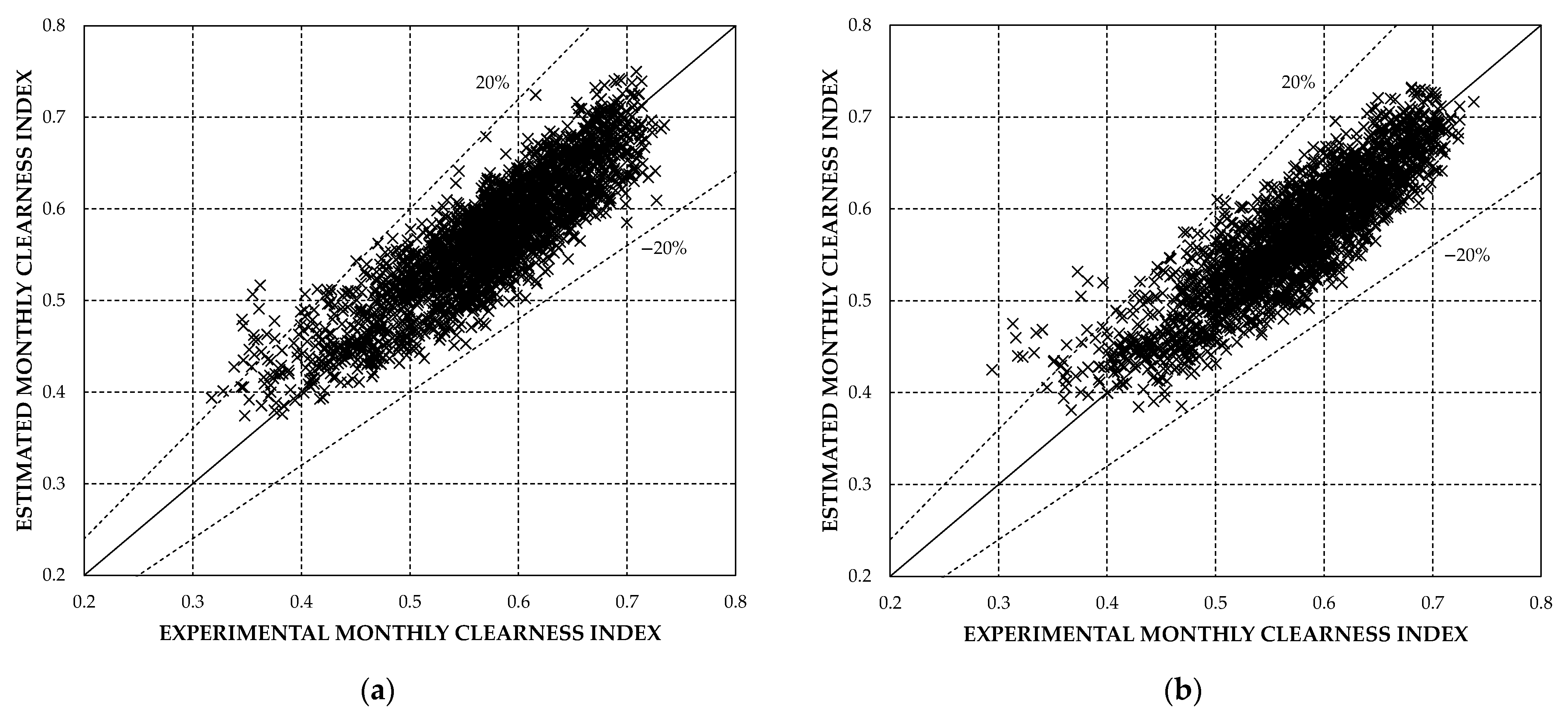
From the figures and tables, it can be deduced that the results are relatively satisfactory for Case 1, with an RRMSE value of 9.28% for the 4968 data set. In addition, with respect to the errors at each station, most of the monthly relative errors are within the range of ±20%, even though the network was trained in this case with less than 13% of the station set.

Table 4. Case 1: Probability that the relative error is greater than a certain x-value and number N of corresponding values.

x (%)	0	1	2	3	4	5	6	7	8	9	10	11	12	13	14	15	16	17	18	19	20	25	30
P (%)	100	91.34	82.63	74.07	64.65	56.98	50.08	43.80	38.53	34.02	30.03	26.43	23.11	19.99	16.43	12.72	9.50	6.94	4.85	3.08	1.85	0.14	0.02
N	4968	4538	4105	3680	3212	2831	2488	2176	1914	1690	1492	1313	1148	993	816	632	472	345	241	153	92	7	1

shows the statistical distribution of the monthly relative errors, with only 92 values above 20%, equivalent to 1.85% of the total data. However, as Figure 6 shows, it is evident that the neural network is biased for many stations in the SIAR network, providing estimates below the experimental data.

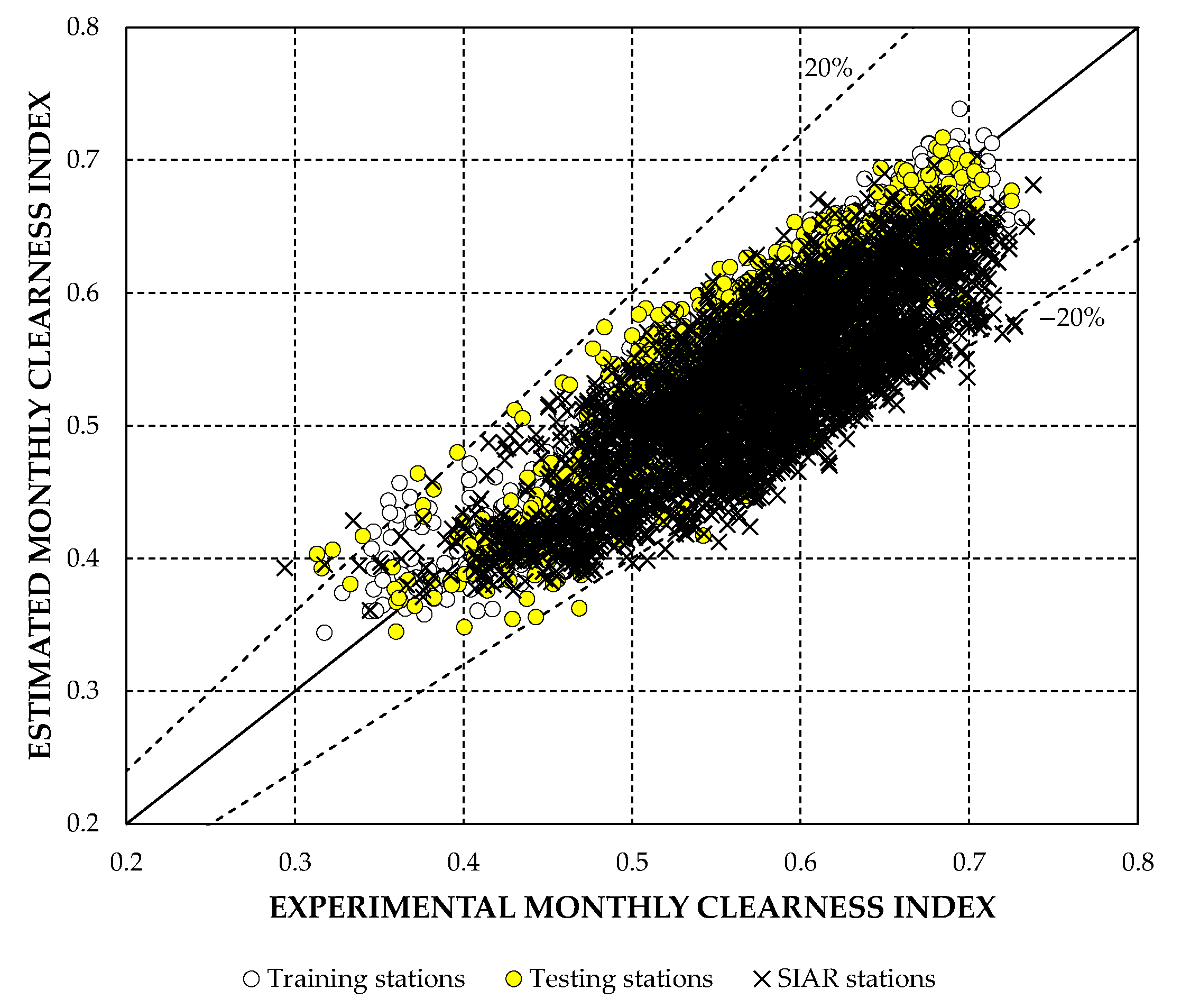
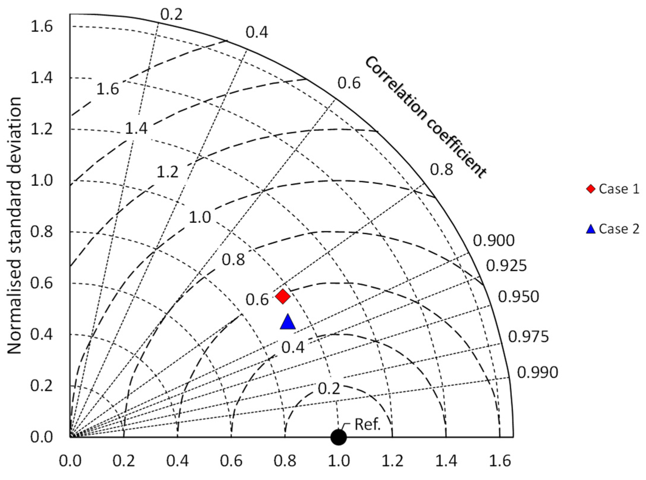
In Case 2, after re-clustering and selection of training stations, an RRMSE value of 6.89% is obtained for the data set. Figure 8 highlights the best statistical indicators obtained in Case 2 for the set of stations. As for the monthly relative errors, the values above 20% are reduced to about half of Case 1, as can be seen from

Table 5. Case 2: Probability that the relative error is greater than a certain x-value and number of corresponding values.

x (%)	0	1	2	3	4	5	6	7	8	9	10	11	12	13	14	15	16	17	18	19	20	25	30	35	40	45	50
P (%)	100	87.24	75.34	64.17	53.10	43.20	34.60	26.99	20.87	15.88	11.74	8.09	6.04	4.39	3.48	2.72	2.19	1.69	1.37	1.19	0.99	0.52	0.34	0.28	0.12	0.04	0.02
N	4968	4334	3743	3188	2638	2146	1719	1341	1037	789	583	402	300	218	173	135	109	84	68	59	49	26	17	14	6	2	1

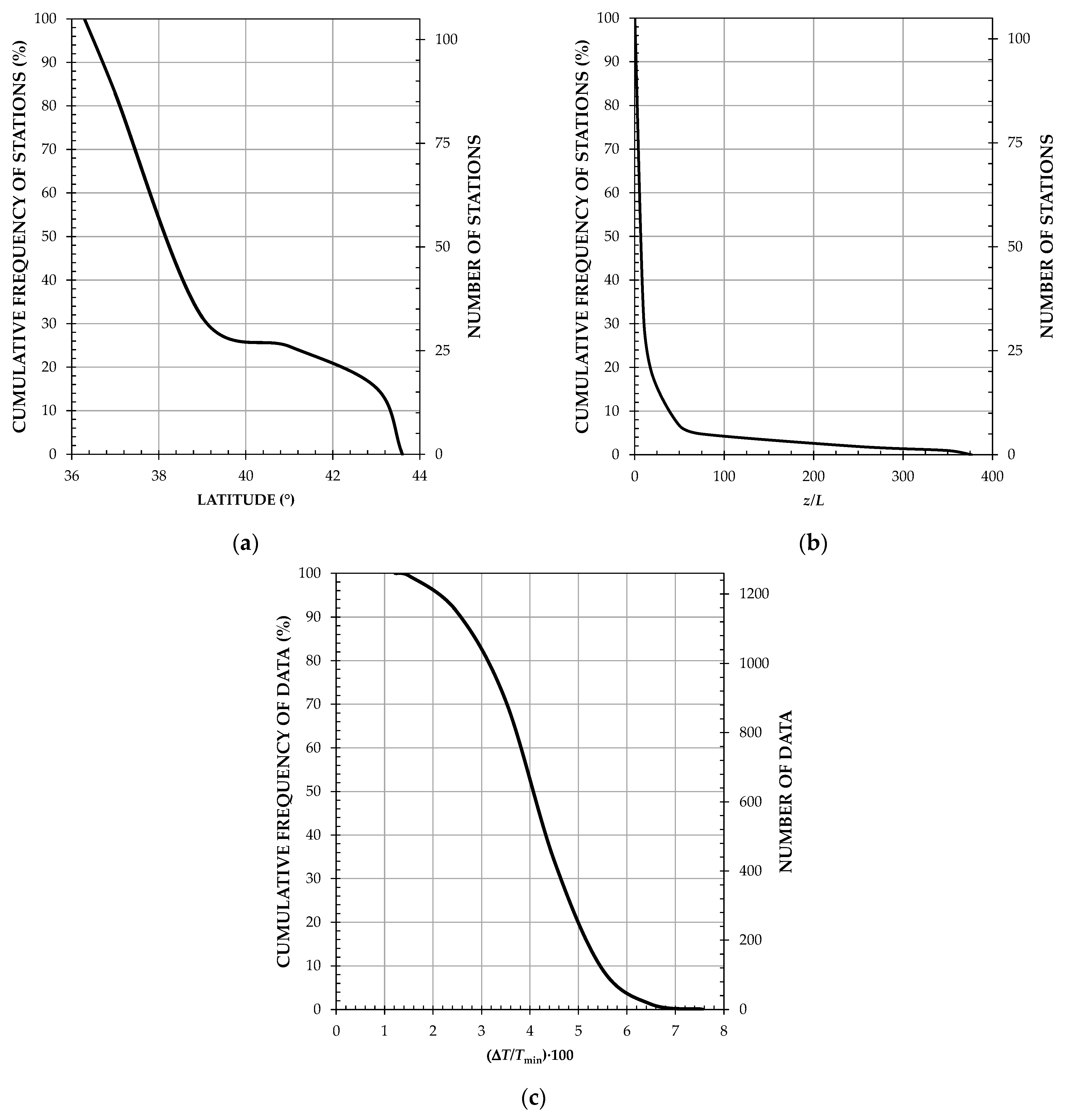
. Figure 9 provides a comparison between the monthly relative error distributions, with a noticeable improvement for Case 2. The comparison between Figure 2a and Figure 3a suggests that the main cause of such an improvement could be the higher percentage of stations used for training in mid-latitudes.

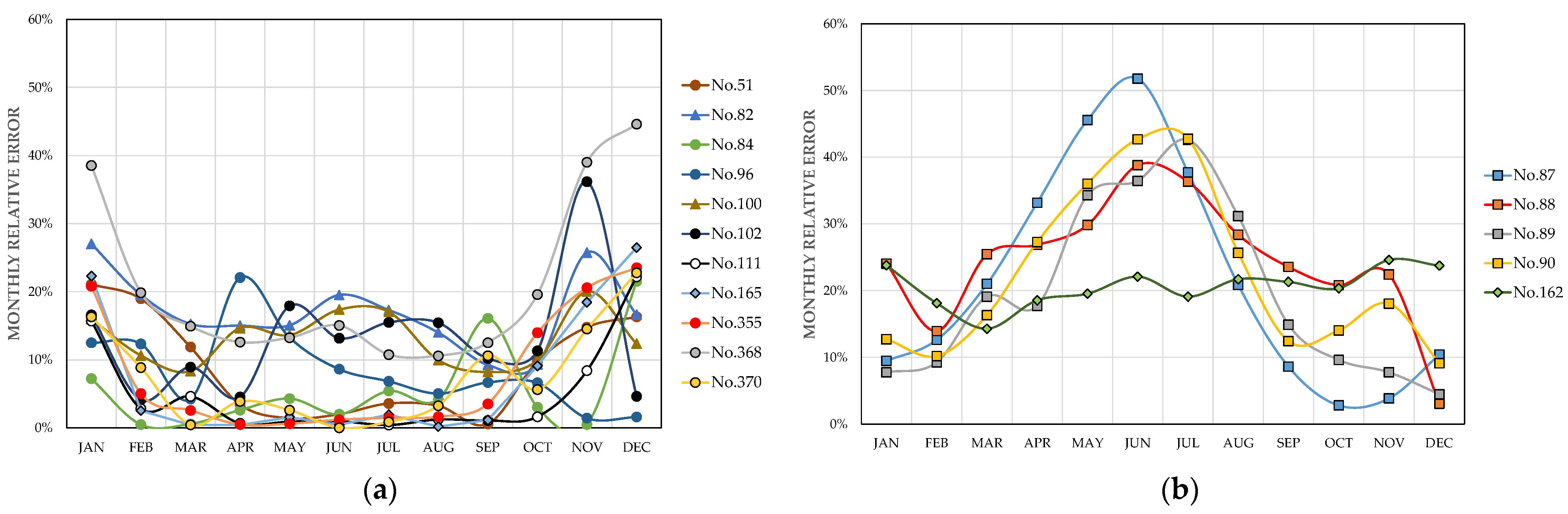
In Case 2 there are 49 values of monthly relative errors greater than 20%, spread over 16 stations. Figure 10a plots the values for the stations where the monthly relative errors are higher than 20% in 3 months at most, while Figure 10b allows comparing the results for the remaining 5 stations where the monthly relative errors are higher than 20% in more than 3 months.

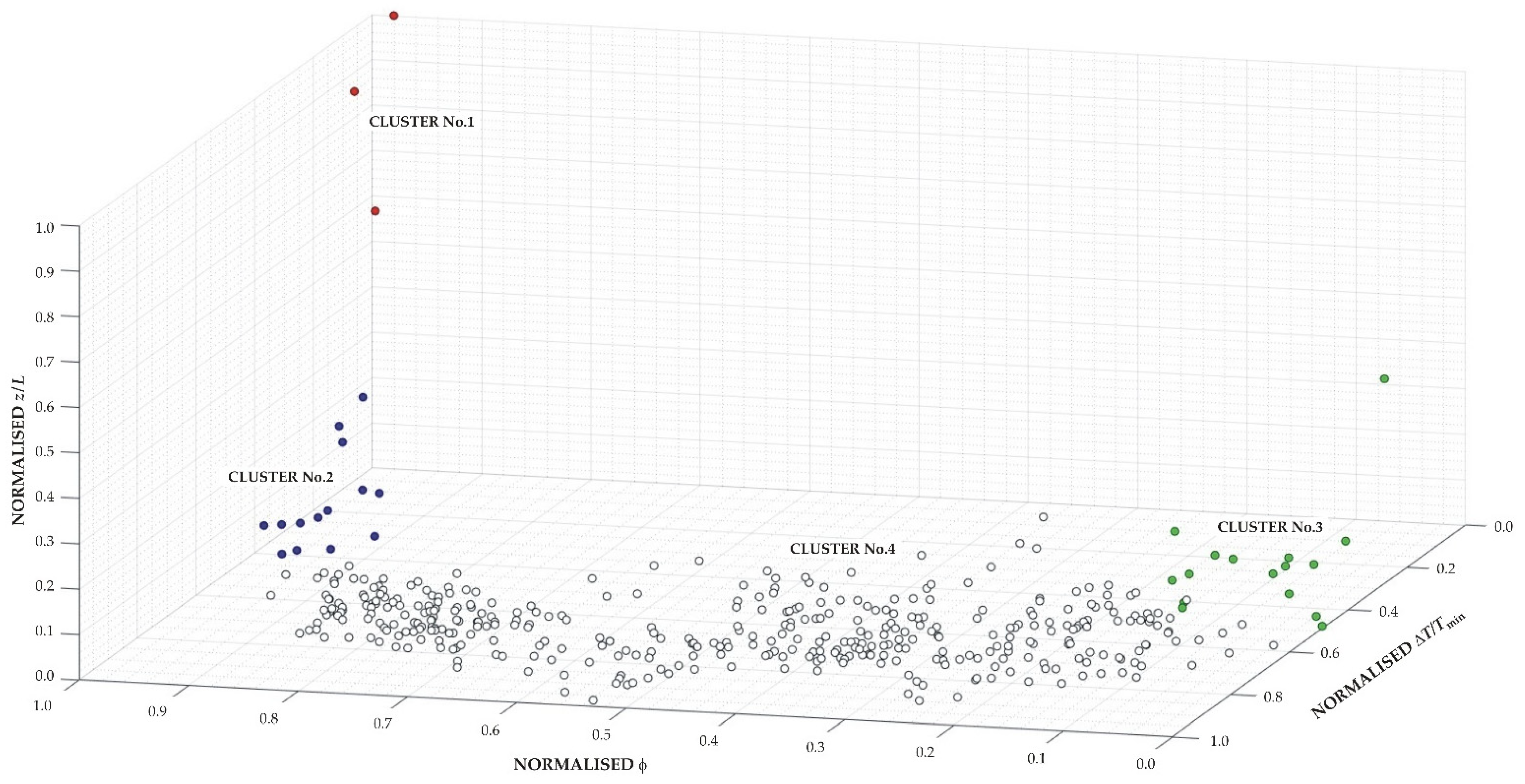
Figure 10a shows that relative error values are higher than 20% in three months at the most for 11 stations, which are included in Cluster No.4, except for station No.100, which belongs to Cluster No.2. For these stations, the least accurate estimates correspond practically to November, December, and January, with the least satisfactory results for station No.368. Figure 10b shows that 25 monthly relative error values are higher than 20% in the spring and summer months for stations No.87–90, while for station No.162, the 7 values of monthly relative error higher than 20% are more moderate and do not have a marked seasonal character. All five stations are classified as Cfb-type climate. Stations No.87–90 are located in a coastal province of northern Spain and are included in Cluster No.2, where high values of latitude and, to a lesser degree of $z/L$ are characteristic. However, station No.162 is located in the Castilian plateau and is included in Cluster No.4. Therefore, it is not evident that the largest errors are associated with high values of such variables since all stations of Cluster No.1 and most of Cluster No.2 present moderate monthly relative errors.

Figure 11a shows the low variability of the monthly clearness index measured for stations No.87–90, with the peculiarity that the difference between the clearness index values in June and December, $∆CI$, is negative. This observation contrasts with the seasonal variability of the clearness index shown in Figure 11b for the remaining 12 stations that also present some monthly error higher than 20%.

Among the 414 stations analyzed, $∆CI$ is negative at only 3 other stations, namely No.85, 91, and 98. Figure 11c shows the variability of the monthly clearness index for these stations, as well as for station No.97, whose data have the lowest positive value of $∆CI$, namely 0.005. This last station and the 7 already mentioned with $∆CI<0$ are included in clusters No.1 and 2, and all of them are in the Principality of Asturias, although managed by different official agencies.

It is interesting to note that in Case 1, stations No.87–90 and 162 also have the highest number of monthly relative errors above 20%. Figure 12 shows that the trends are similar in both cases but with more moderate errors in Case 1.

Furthermore, it should be noted that data from stations No. 1–71, located in southern Spain, were used in previous work to compare 14 GSR models based on regression and temperatures [12]. To evaluate their use as general models, the fit coefficients were replaced by functions of the $z/L$ ratio. The best averages for the set of stations, $RRMSE=7.45\%$ and $R^2=0.9693$, were obtained using the modified Adaramola model [12,34], which expresses the clearness index by a linear function whose only variable is the monthly average daily mean temperature. This model predicted annual mean errors of less than 20% for all stations except for station No. 24, located in Cádiz, where the error was 50.32%, the most probable cause being that the $z/L=150$ value at this location is notably higher than at the rest of the stations. Given that ANN predicts for station No.24 annual mean errors of 2.76% in Case 1 and 6.63% in Case 2, it can be concluded that the probability of obtaining unacceptable estimates at the local scale is lower using the neural network-based procedure.

As a complement to the analysis carried out for the Spanish stations and as a preliminary step to more comprehensive future work, the performance of the neural network has also been evaluated using data from stations located in other countries.

Table 6. Monthly clearness index, geographical and climatic data for non-Spanish stations [14].

No.	Location	$\mathit{\varphi }\mathbf{(}\mathbf{°}\mathbf{)}$	$\mathit{z}/\mathit{L}$	KGCC	JAN	FEB	MAR	APR	MAY	JUN	JUL	AUG	SEP	OCT	NOV	DEC
415	Ahar (Azerbaijan)	38.43	8.763	Csa	0.5433	0.5791	0.5644	0.5679	0.6035	0.6391	0.6491	0.6430	0.6437	0.6243	0.5596	0.5372
416	Bragança (Portugal)	41.82	4.035	Csb	0.4478	0.5464	0.5346	0.5781	0.5941	0.6427	0.6792	0.6673	0.6418	0.4974	0.4678	0.3889
417	Çannakkale (Turkey)	40.13	15.789	Csa	0.3427	0.3613	0.4481	0.4965	0.5373	0.5657	0.5977	0.5683	0.5462	0.4774	0.4051	0.3306
418	Elkins (USA)	38.88	2.096	Dfa	0.4129	0.4294	0.4643	0.4565	0.4869	0.4937	0.4794	0.4921	0.4801	0.4513	0.4261	0.4135
419	Faro (Portugal)	37.02	11.887	Csa	0.5754	0.6196	0.6209	0.6563	0.6645	0.6934	0.7082	0.6847	0.6616	0.6302	0.5972	0.5324
420	Isparta (Turkey)	37.85	10.324	Csb	0.4680	0.4699	0.5100	0.5246	0.5660	0.6105	0.6340	0.6104	0.6329	0.5477	0.5224	0.4554
421	Monte Real (Portugal)	39.83	5.844	Csb	0.5307	0.5019	0.5701	0.5707	0.5837	0.5795	0.6424	0.6464	0.6138	0.5783	0.5623	0.5323
422	New York JFK (USA)	40.65	2.275	Cfa	0.4001	0.4715	0.4911	0.4691	0.5034	0.5159	0.5111	0.5878	0.5047	0.5835	0.4591	0.4057
423	Pocatello Airp. (USA)	42.92	1.440	Dfb	0.4682	0.5359	0.5420	0.5854	0.5726	0.6337	0.6550	0.6644	0.6413	0.6167	0.4901	0.4647
424	Roma-Ciampino (Italy)	41.80	5.984	Csa	0.4059	0.4596	0.5008	0.4791	0.5176	0.5428	0.5673	0.5484	0.5079	0.4748	0.4003	0.3598
425	San Francisco (USA)	37.62	41.667	Csb	0.4616	0.5287	0.5594	0.5824	0.5814	0.6174	0.6290	0.6224	0.6338	0.5702	0.5108	0.5033
426	Sendai (Japan)	38.27	5.402	Cfa	0.4943	0.5067	0.4834	0.4840	0.4353	0.3642	0.3380	0.3779	0.3698	0.4353	0.4651	0.4795
427	Sofia (Bulgary)	42.68	2.754	Cfb	0.3446	0.4166	0.4244	0.4209	0.4542	0.4926	0.5064	0.5030	0.4600	0.4150	0.3590	0.2905
428	Turpan (China)	42.93	0.016	BWk	0.4676	0.5407	0.5500	0.5700	0.5753	0.5593	0.5497	0.5615	0.5933	0.5820	0.5127	0.4401
429	Viterbo (Italy)	42.43	7.815	Csa	0.4728	0.5214	0.5356	0.5073	0.5714	0.5937	0.6205	0.6087	0.5566	0.5214	0.4765	0.4307
430	Yinchuan (China)	38.48	1.106	BWk	0.5943	0.5999	0.5671	0.5743	0.5836	0.5556	0.5441	0.5425	0.5528	0.5779	0.5874	0.5804

shows the data of the monthly clearness index for 16 non-Spanish stations with input variables within the following ranges:

$$0.020\le ∆T/T_{\mathrm{m}\mathrm{i}\mathrm{n}}\le 0.067$$

$$37.02°\le \varphi \le 42.93°$$

$$0.016\le z/L\le 41.667$$

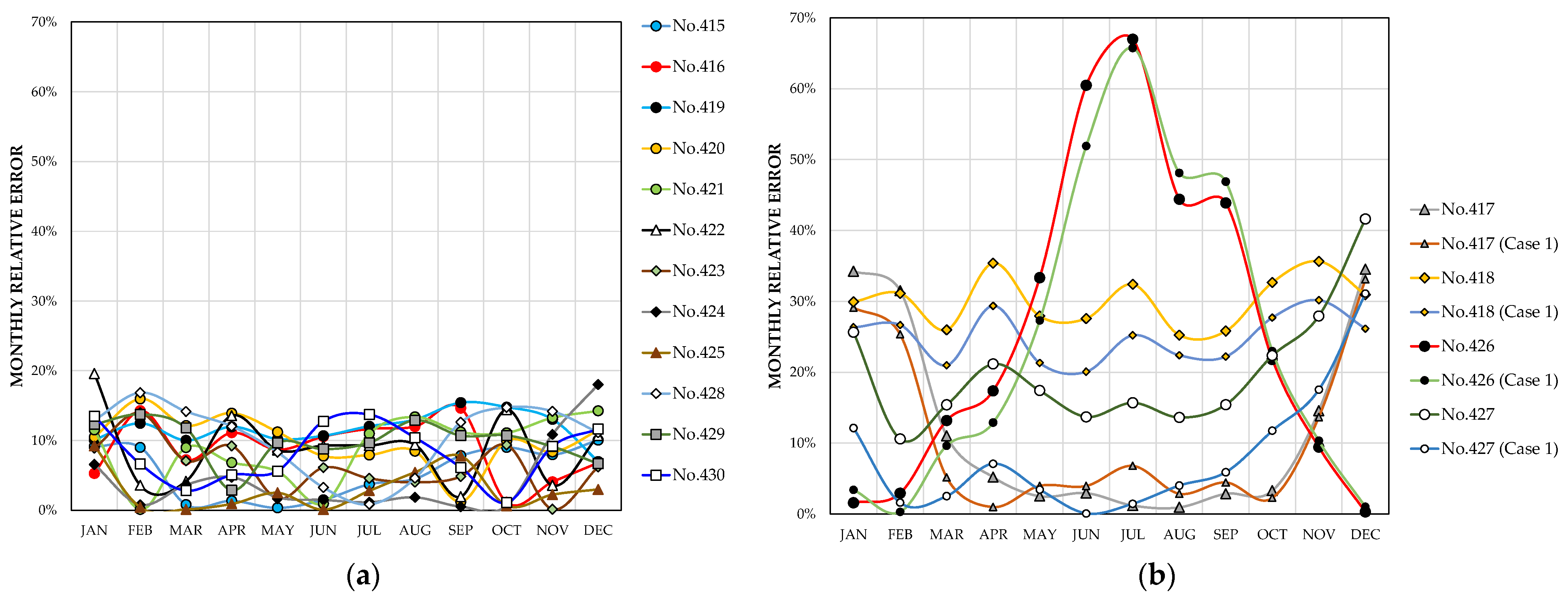
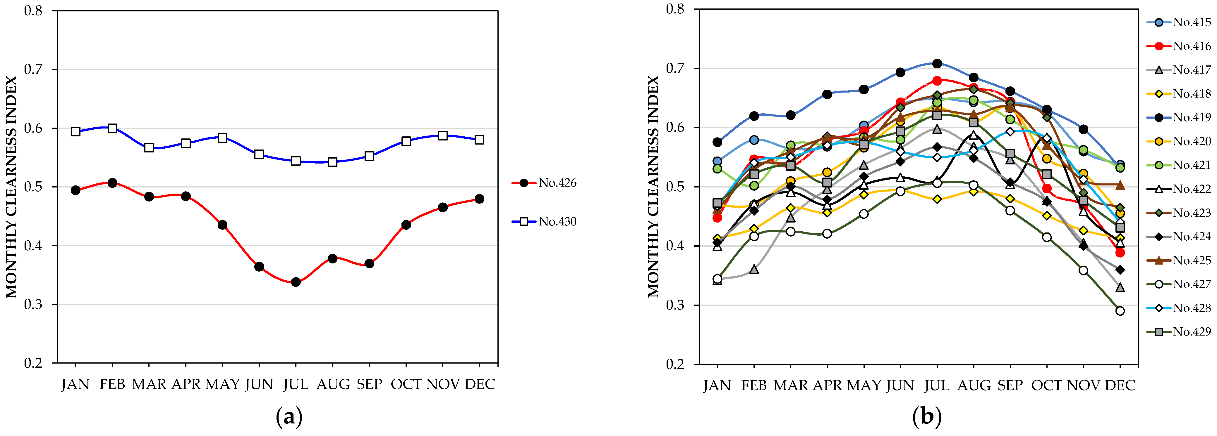
As shown in Figure 13a, using the neural network trained in Case 2, the relative error of the clearness index is less than 20% for 12 stations during all months of the year. For the remaining four stations, Figure 13b shows that the monthly relative errors are greater than 20% for station No.418 in all months of the year, with no appreciable seasonal differences. This result seems to be justified mainly because this station has a Dfa climate in the Köppen–Geiger classification and there are no stations of this class among the 414 Spanish stations analyzed. The errors are highest for station No.426 in the spring and summer months, while the highest errors are observed from December to February for station No.417 and from October to January for station No.427. Figure 13b also shows that the same stations present the highest errors and with similar monthly trends when estimates are made using the neural network trained in Case 1, although the errors are more moderate except for station No.426. It can be interpreted that the remarkably high errors obtained at this station are related to the negative value of $∆CI$, as Figure 14a shows. On the contrary, Figure 14b shows that stations No.417 and 427 have similar clearness index trends to the stations with lower errors, which is consistent with the fact that the errors at these stations only exceed 20% in 3 and 1 months, respectively, when using the network trained in Case 1.

The difference between the June and December clearness index is also negative for station No.430, located in Yinchuan, China, with some similarity to the behavior represented in Figure 11c for stations No.85, 91, 97, and 98 on the Spanish north coast, and also with acceptable monthly errors. However, the ANN estimates for station No.430 are pending corroboration because, among the 414 Spanish stations analyzed, there is only one with the same BWk type climate, namely station No.1, located at the Plataforma Solar de Almería facilities, in the desert area of Tabernas.

In summary, it can be said that the choice of the best model is a matter of preference between objectives: The behavior of the ANN in Case 2 is more appropriate if the objective of obtaining the lowest mean error for the set of stations is a priority, but Case 1 leads to more moderate values of the maximum monthly relative errors, with a mean error for the set of stations that can be considered acceptable, especially if one takes into account that in this case the network has been trained with less than 13% of the set of stations.

In any case, the less accurate estimates seem to be related to climate types where the clearness index tends to be higher in winter than in summer, which is the case in few locations on the northern Spanish coast. This result is consistent with the estimates obtained for the Japanese locality of Sendai and suggests that the sign of the difference between the clearness indices in June and December may be a basic indicator of climatic variability as a complement to the Köppen–Geiger classification.

Future work is expected to improve the ANN model, designed to estimate GSR over large regions and based on temperature and geographic input data, using algorithms that incorporate climate variability as a variable for selecting training weather stations.

5. Conclusions

Hierarchical clustering, based on normalized values of relative temperature amplitude, latitude, and the ratio of elevation to distance to the sea, is suitable for the characterization of solar radiation data.

A simple ANN is capable of estimating GSR from temperature, orography and geography data with acceptable accuracy, both with respect to error averages for the input data set and with respect to local errors, which is interesting for low-cost solar resource assessments over wide areas.

The application of Buckingham’s theorem to the functional relation underlying the ANN simplifies the structure of the ANN, providing computational advantages due to the smaller number of variables and weights.

The percentage of data used for ANN training influences the quality of the results. In this work, with the same network structure, a lower average error was obtained for the set of 4968 data measured at 414 Spanish stations using 50% of the data for network training, but local errors were lower using 18% of the data for training.

The results of the article once again corroborate the usefulness of the $z/L$ ratio as a proxy for both elevation and thermal regulation of the sea.

The ANN trained with data from Spanish stations performs generally well for other places all around the world within the same ranges of input variables.

The difference between the clearness indices in June and December could be used in the hierarchical clustering of climate data as a complement to the Köppen–Geiger classification, which is suggested to be studied in future works.