Optimization Algorithms for Sustainable Operation of Multi-Unit Hydropower Plants

Abstract

The work presented in this article concerns numerical studies on optimization methods used for the sustainable utilization of the energy potential of water, converting it into electricity in a hydropower plant equipped with more than one unit. These methods allow for maximization of production in given hydrological conditions, leading to the balanced, lossless, and environmentally friendly use of the renewable energy source that is water. Methods are selected from three groups, i.e., analytical, enumeration, and randomized. The results of calculations of optimal points of selected test functions carried out using the Broyden–Fletcher–Goldfarb–Shanno Limited-Memory Version (L-BFGS-B), Explicit Complete Enumeration (ECE), and Genetic Algorithm (GA) methods provided basic information on the features of these methods. Based on these tests, the GA method was selected to solve the problem of the optimal load distribution in a hydropower plant equipped with three identical hydro units. The defined optimization problem consisted of finding a configuration of hydro units in operation that would guarantee the maximum efficiency of the power plant under the imposed hydrological conditions. During the numerical studies, a number of calculations were performed to identify the impact of procedures and parameters characteristic of the optimization methods on the obtained results. Particular attention was paid to the GA method and penalty functions, enabling the elimination of results from the area of prohibited solutions.

1. Introduction

The idea of sustainability in the era of intensification of unfavorable climate changes requires the protection of natural resources, including the optimal use of their energy potential. This also applies to water resources, the protection of which means the need to develop a network of structures for water retention, purification, and reduction of waste, as well as the need to equip hydropower plants with highly efficient units using all of the available energy potential, which means using it in an optimal way. Maximum use of the energy potential of water flowing in the river must respect all the rules applicable to the system in which the hydroelectric facility operates. This includes the need to secure the needs of all users of water resources, and, above all, the needs of the natural environment, such as securing inviolable flows, watering natural riverbeds and wetlands, and operating fish passages. This means that hydroelectric facilities should be able to preserve biodiversity and maintain the required hydrological conditions in the area of the power plant’s impact on the environment. The use of the remaining available potential intended for energy production imposes an obligation or even a moral imperative to utilize this potential in such systems to the greatest possible extent. This should lead to the use of modern machines, manufactured using environmentally friendly technologies and operated according to optimal settings that guarantee maximum efficiency as well as minimum wear and failure rates. However, such a solution requires the use of appropriate optimization methods in the planning, design, and operation stages of the hydropower plant. The effect of such actions is also an increase in the profitability of hydropower plants, which in the case of the building phase is characterized by significant investment outlays, which is always a huge challenge.

The rationalization of generating equipment settings in hydropower plants, naturally and directly connected with the optimization of their operation, is a low-cost method of increasing the production of electricity. Additionally, it also allows for extending the service life of hydro units. This is achieved by reducing dynamic loads by shifting the operating point of the machines to an area of higher efficiencies, which is also characterized by lower vibrations and pressure pulsations. In terms of maximizing production in hydropower plants, the following can be distinguished:

• individual optimization of hydro units operating in the power plant, possible in the case of hydro units with a double or higher degree of regulation (e.g., equipped with a Kaplan or Deriaz turbine or a variable rotational speed system),
• group optimization of two or more hydro units in a given power plant,
• group optimization of cooperating power plants, e.g., operating as part of a river cascade.

If the hydro units being optimized have a double or higher degree of regulation, they should always be individually optimized before implementing group optimization. In turn, the group optimization of several power plants should be preceded by the group optimization of the hydro units operating in each of these power plants. Fulfilling these conditions is necessary to obtain the desired effect in the form of maximizing the use of the hydropower potential available in the whole water system where hydropower plants are operated. This is extremely important in the context of searching for solutions that must meet the needs of the development of distributed power generation. The structure of modern and ecological power generation based on renewables requires that devices optimally use resources while maintaining the idea of sustainable development.

In addition, optimization issues require taking into account several conditions. In the case of individual optimization of the hydro unit, limitations such as turbine and generator characteristics, range of operational load, etc., should be considered. On the other hand, for the issue of group optimization, it is usually required to take many criteria into account (from maximizing efficiency to maximizing revenues from energy sales and minimizing the impact of the power plant’s operation on the environment), as well as limitations related to the use of hydro units, such as:

• limitations resulting from hydrological conditions and hydro-technical characteristics of the structures, including their safety and stability,
• restrictions resulting from formal and legal conditions, such as legal water permits and a water management plan,
• obligations to other users of the river or water reservoir used for energy production.

Many publications on this subject present comprehensive reviews of methods used to optimize the operation of renewable sources, particularly hydropower plants [1,2,3,4,5,6]. This paper focuses on the group optimization of hydro units operating in a given power plant, where the criterion is to maximize the efficiency of the entire power plant. The problem comes down to finding a distribution of hydro unit loads that will ensure maximum electricity production in the power plant under given hydrological conditions. Many publications are addressing the topic of optimal load distribution in hydropower plants equipped with multiple units. Works presented in these publications focus on researching and proposing various calculation methods. In the paper by Arce et al. [7], a model for the operation of 18 hydro units in the Itaipu power plant was described, based on the dynamic programming technique used for minimizing costs of start-up or shut-down unit cost, as well as power generation loss unit cost. In [8], the authors presented a model using the heuristic-based combinatorial optimization technique, which was applied to optimize a hypothetical power plant equipped with two or more hydro units. A paper [9] presents the problem of appropriate formulation of optimization of the hydropower plant operation and its influence on the obtained calculation results in an example hydropower plant with six units equipped with different types of water turbines. In [10], a dynamic unit commitment and loading model used for determining the hydro unit generation schedules at BC Hydro is presented. Many of the papers deal with the problem of load distribution in a single power plant equipped with more than one unit, presenting analyses of various optimization methods carried out based on real facilities [11,12,13,14,15,16,17,18,19]. For example, in [11], the authors define the unit optimal commitment of a single hydropower plant as a nonlinear integer-mixed problem and propose an algorithm based on branch and bound and projected gradient methods for its solution. In turn, in [12], the modified shortest path algorithm is chosen to show multiple optimal solutions for the case study of China’s Geheyan hydropower plant that are useful to assess the highest efficiency together with low vibration conditions of hydro units.

Due to the different levels of complexity, the optimization problems also differ from each other in the level of difficulty of finding a solution. Therefore, for each of these problems, an appropriately matched algorithm is sought, which allows for the most accurate determination of the optimal solution at the lowest possible cost (acceptable computation time). This requires thorough knowledge of the analyzed problem and knowledge of the basic features of the optimization methods used. Such knowledge is a condition for achieving satisfactory results, and a lack of this knowledge may lead to failure to obtain results or, even worse, to incorrect optimization results.

The work presented in this paper concerns the following:

• Analyses and assessment of optimization methods selected from three groups of methods: analytical, enumeration, and randomized. They were based on detailed testing of representative algorithms consisting of calculating the extremes of selected test functions.
• Selection of the appropriate method to solve the problem of load distribution in a hydropower plant equipped with three units. Further tests using a suitably formulated optimization problem focused on the appropriate definition of conditions preventing results from being obtained were placed in prohibited areas of the solution domain.

The main contribution follows from the results of the works that were used to indicate the procedures and their parameters, which are important for obtaining a tool that provides reliable results when searching for solutions to maximize production in hydropower plants equipped with several units. The most attention was paid to the internal procedures of the GA method and the penalty procedures, which allow for the elimination of solutions from the prohibited area. This issue is one of the most important in practice for methods of searching for the optimal distribution of loads between the hydroelectric power plant units. The authors present a possible solution to this problem through an in-depth analysis and tests.

If optimization aims to achieve the goal of utilizing the available energy potential of water while meeting the needs of other users, including, above all, securing the needs of the natural environment and hydrology, it becomes the basis for a balanced and environmentally compliant solution for hydropower plant operation. Therefore, implementation of such optimization is one of the most important elements of achieving sustainable management of water resources in the systems where the hydroelectric facility is located. This paper indicates possible directions for further work on such issues.

2. Optimization Problem and Methods of Solution

Optimization is the process of searching for the best solution to a given problem, based on the adopted evaluation criterion and taking into account the adopted constraints. The correct formulation of an optimization problem includes:

• a function of one or more variables, called the objective function:

  $$F_{obj}=f\left(x_1,x_2,\dots ,x_n\right)\to \mathit{max}\hspace{1em}\mathrm{o}\mathrm{r}\hspace{1em}min$$

  (1)

  which reaches an extremum (maximum or minimum) for the sought values of decision variables $x_1,x_2,\dots ,x_n$.
• a set of constraints $u$ in the form of a system of $m$-equations or inequalities (a system of constraints):

  $$u_i\left(x_1,x_2,\dots ,x_n\right) \mathrm{f}\mathrm{o}\mathrm{r} i=1,\dots ,m$$

  (2)

  which must be met by the decision variables $x_1,x_2,\dots ,x_n$.
• boundary, initial, and final conditions:

  $$\begin{gathered} X_i^{min}\le x_i\le X_i^{max} \\ {x}_i\left(t=0\right)=X_i^0 \\ {x}_i\left(t=T\right)=X_i^T \end{gathered}$$

  (3)

  where $T$ is the time at the final condition.

As this paper addresses the optimization of electricity generation from multiple-unit hydroelectric power plants to maximize efficiency (maximize energy production and minimize water use), the constraints are related to meeting environmental and operational constraints (e.g., flow rate limitations, environmental regulations, and machine limitations). For such tasks, the definition of the optimization problem will certainly be characterized by a complex objective function and a fragmented area of permitted solutions. Due to this, an appropriate method for solving such problems is needed. In the case of the optimization problem defined in Equations (1)–(3), an algorithm based on one of the three main types of methods can be used, i.e., analytical, enumeration, or randomized.

In analytical methods, the extremum of the objective function can be sought by moving in the direction determined by the gradient (a derivative of the objective function), or by solving a system of equations obtained by equating the gradient to zero. Analytical methods are characterized by their very short calculation times and provide precise, accurate solutions. However, due to the need to calculate derivatives of the objective function, this function must meet the following criteria, i.e., it must be continuous and differentiable.

Enumeration methods are based on calculating the value of the objective function in the entire domain of solutions and choosing its extremum value as the final solution. These methods have a very simple idea of conducting calculations and do not require the condition of smoothness or the existence of derivatives of the objective function. As a result of their use, a global extremum is always obtained. However, these methods are inefficient for large solution areas, and the final solution, because it is correlated with the resolution of the results (the size of the step along one of the domain axes with which it is “sliced”), may be inaccurate. The increase in accuracy, requiring an increase in resolution (reducing the previously mentioned step between “slices”), is sometimes associated with a dramatic increase in computational costs by extending the computational time or utilizing appropriately large amounts of computing power.

Randomized optimization methods, as the third of the above-mentioned groups, consist of randomly examining the entire solution domain and searching for the best value (global maximum or global minimum) of the objective function. Similarly to enumeration methods, in random methods, the objective function does not have to be smooth or differentiable. The computation time increases with increases in the solution area. However, these methods are much faster than enumeration methods and, additionally, the loss of efficiency with the increase in resolution or solution area can be significantly reduced by using additional numerical tools. One of the shortcomings of randomized methods is the possibility of converging to a local, not global, extremum. However, the probability of this is much lower than in analytical methods. The obtained solutions may be imprecise and reducing this problem requires careful design of all the procedures accessible using these methods.

Each of the groups of methods mentioned and briefly characterized is intended as a tool for appropriate optimization tasks. Through knowledge and proper control of their parameters, algorithms dedicated to issues encountered in engineering practice can be created.

3. Tests

As part of the work aimed at developing an appropriate tool useful in the area of optimizing the operation of hydropower plants, several tests of optimization algorithms were carried out. The tests were based on two functions that are very different from each other. The choice of these functions was dictated by the need to ensure that the criterion for using the analytical method was met. Therefore, the test functions are differentiable and continuous in the solution area. However, it should be remembered that, in practice, the objective functions that meet these criteria are rarely found, and certainly not in the entire solution domain. The results obtained using the algorithms were compared in terms of the quality of the results and the time of the calculations (the number of performed calculation iterations). The algorithms of the selected methods were programmed in the Visual Studio Community environment in C++. The following methods were selected for testing:

• Broyden–Fletcher–Goldfarb–Shanno Limited-Memory Version (L-BFGS-B)—representing analytical methods,
• Explicit complete enumeration (ECE)—representing enumeration methods,
• Genetic algorithm (GA)—representing randomized methods.

Among the selected algorithms, those are representatives of different methods of solving optimization problems. Each of the methods has slightly different characteristics and is suitable for different types of problems. Thanks to the detailed testing of these algorithms on problems with different characteristics, features focusing on their ability to deal with complexity, uncertainty, or real-time constraints were confirmed. The details of the selected methods are described below.

3.1. Tested Optimization Methods

3.1.1. L-BFGS-B Method

The L-BFGS-B method is a gradient method [20]. This means that the actions aimed at finding the extremum of the function are based on tracking the gradient, i.e., the derivative of the objective function (the objective function reaches the extremum when its derivative takes the value 0). The program uses the publicly available DLib library [21], which is distributed based on open-source licensing and contains, among others, an implementation of the L-BFGS-B method. This is a method that allows users to avoid collecting full data on changes in the gradient of the function in the solution area. It is based only on the gradient determined in the previous calculation step. This makes this method less cost-intensive compared to other gradient methods and therefore useful in the optimization of multivariable functions.

From the characteristics of analytical gradient methods, it follows that their basic limitation is the requirement for a continuous and differentiable objective function. This is a significant limitation when using these methods in practice. In addition, these methods can converge to local extrema, which is directly connected with the initial point from which the search for the global extremum begins (Figure 1). Despite the limitations of using these methods in practice, they constitute the basis of numerical algorithms and can successfully be an element of hybrid algorithms, in which analytical methods can support other types of optimization methods.

In the example of the calculation process of the optimization algorithm based on the gradient, shown in Figure 1, it is visible that the choice of four different starting points can significantly differ in the final result of the operation. Only in the case of starting points #3 and #4 will the algorithm, which always follows the direction in which the derivative of the objective function is negative ($dF\left(x\right)/dx<0$), converge to the global extremum located at point $x_j$. Moreover, the choice of the starting point also determines the speed of finding the solution. In the case of starting point #4, the solution is found in the shortest time (in three calculation steps). During tests of this method, the program randomly set the starting point when searching for the extremum. The analysis took into account the accuracy of the solution for the calculation cycles carried out for 200 different starting points.

3.1.2. ECE Method

For tests, the ECE algorithm was used [22], in which the search for the extremum consisted of determining the value of the objective function in the entire solution domain. It follows a simple algorithm that reads the values of the objective function on consecutive levels. “Cutting” the function into “slices” ensures the gathering of values of the function at the given levels. Comparing these values with each other allowed the global extremum to be found. The search for the entire solution area was performed with a specified resolution (step between the “slices”) and the computational time at different resolutions and sizes of the solution domain was analyzed. 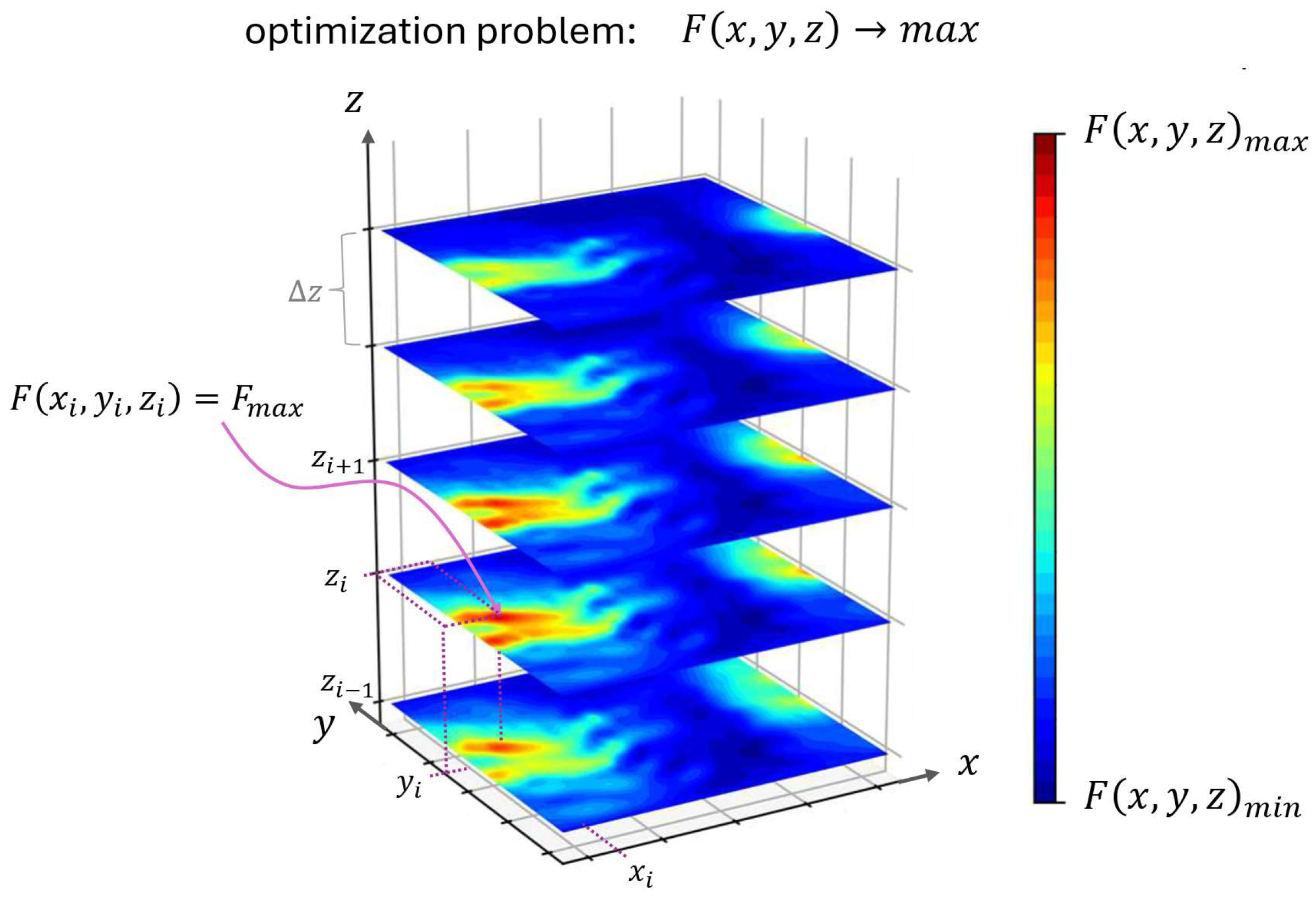Figure 2 shows an example of searching for the maximum of a 3D function. The resolution of the ECE method is defined by the step $∆z$. As can be seen, after scanning the entire solution domain and comparing all obtained values of the $F$ function, its maximum was found in the $i$-th step, i.e., at the point with coordinates $\left(x_i,y_i,z_i\right)$.

Since the actual maximum of the function may lie between steps $\left(i-1\right)$ and $\left(i+1\right)$, the accuracy of the ECE method is expected to depend on the imposed resolution. This resolution will also affect the computational time. Another limitation of this method follows from the necessity to scan all of the solution area before finding the extremum, which can additionally extend the calculation times.

3.1.3. GA Method

The genetic algorithm was chosen as a representative of randomized methods. This algorithm has found many applications in the search for optimal solutions, including in engineering practice. Therefore, it is widely described in the literature. There is a large database of monographs dealing with this topic, etc. [24,25]. The GA method, in the process of searching for the solution area, uses a method analogous to the processes of natural evolution, the aim of which is to optimally match individuals to existing environmental conditions. In this analogy, individuals are vectors of decision variables, which are the coordinates of the points of the solution domain (Figure 3). They are subject to encoding, e.g., using the binary system, which generates the genes making up an individual (often called a specimen or chromosome).

The genetic algorithm generates an entire population of individuals through the selection and manipulation of genes. Each individual in the population differs from the others in terms of the configuration of genes, which means that it represents a specific point in the solution area with a unique combination of coordinates. In the next steps, the algorithm compares the values of the fitness function $F_f$ for each individual, which is a quantitative analogy to the quality of the adaptation of a given individual to the environmental conditions obtained in the process of natural evolution. The value of $F_f$ takes into account all the constraints imposed on the decision variables and the characteristics of the objective function defined for a given optimization problem. 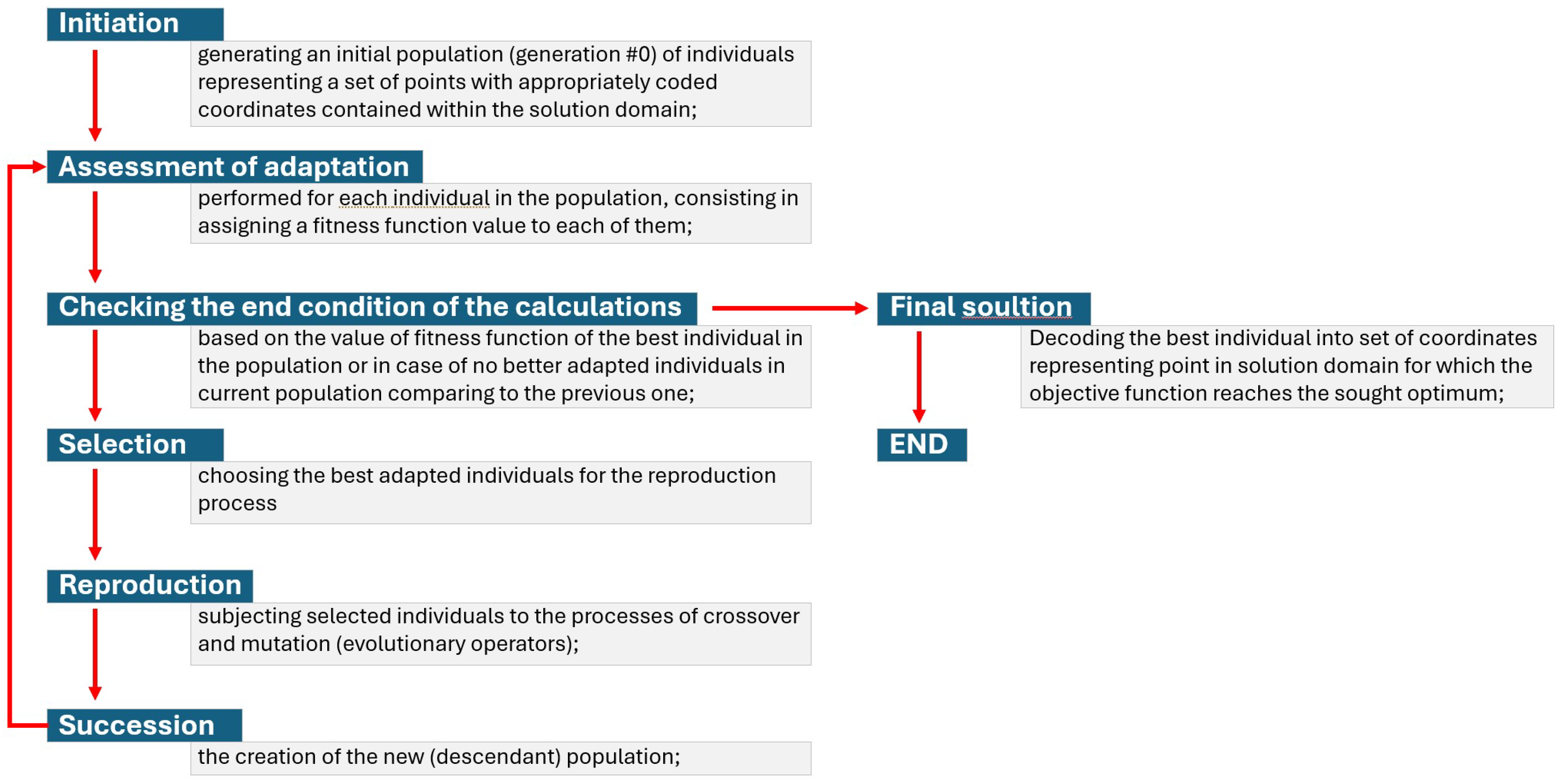In this way, the value of the function $F_f$ can be used to obtain information about the proximity of a given point to the optimal solution sought. By applying successive procedures reflecting processes encountered in nature, such as the selection of individuals or gene crossovers and mutations, a descendant population is generated from the initial one, consisting of new individuals that inherit genes from individuals from the previous generation (parents in the previous population). This process is repeated until an individual with the sought adaptation, representing the optimal solution to the posed problem, is obtained. The flowchart of the genetic algorithm is shown in Figure 4. Each passage of the loop between the assessment of adaptation and succession constitutes another iteration of the GA calculations.

Each of the presented steps of the GA can have a significant impact on its operation and efficiency. In this work, the analysis of this issue covers:

• Different methods of encoding individuals:
  The analyses considered two methods of encoding used to represent points (individuals) of the solution area: natural binary encoding [26] and Gray encoding [27]. Natural binary encoding does not always ensure that two points that lie close to each other in the solution area also lie close to each other after coding. A good example is the numbers 7 and 8, which in natural binary encoding have the form 0111 and 1000, respectively. As can be seen, these two adjacent numbers differ in all digits in the natural binary notation. Therefore, it is obvious that the probability of obtaining these values using such a coding method is very low. To avoid such situations, the Gray scheme is often used, in which neighboring numbers differ only by one digit in the binary notation. For example, the numbers 7 and 8 in the decimal system are represented as 0100 and 1100, respectively, so they only differ by one digit.
• Different methods of selecting individuals for further reproduction:
  Three different methods of selecting individuals for the construction of descendant populations are analyzed [24,25]:
  • Roulette Wheel Selection—consists of drawing individuals after assigning each of them to a section of the roulette wheel that corresponds to the quality of its adaptation;
  • Tournament Selection—consists of selecting the best-adapted individual from a specified number of individuals drawn for the tournament;
  • Rank Selection—consists of sorting the individuals of the population from the most to the least adapted and selecting only a specified number of individuals with the best adaptation from such series.
• Application of different probabilities of occurrence of crossover and mutation:
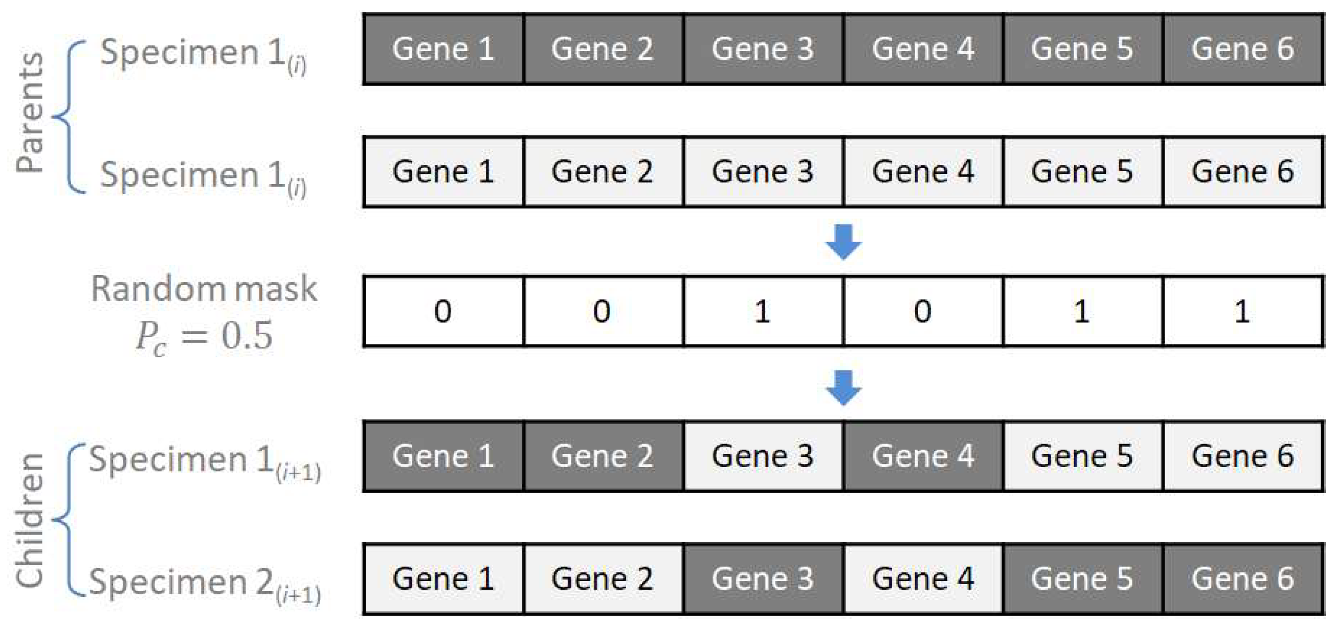
  In the tested program based on the GA method, the crossover procedure consists of exchanging individual genes passed on by parents to descendants by randomly selecting them with the assumed probability $P_c$. In cases where this probability is different from 0.5 (Figure 5), descendants have more genes originating from one of the parents.
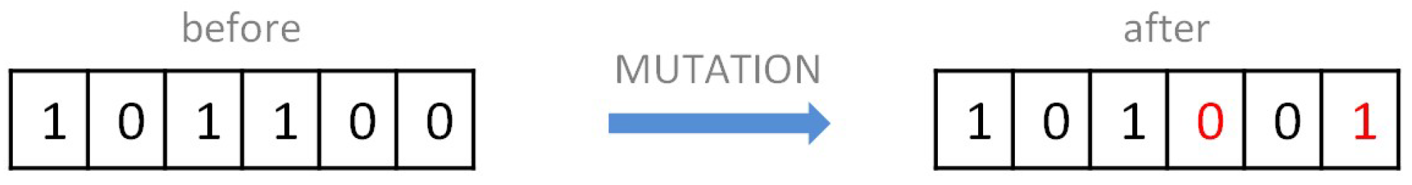
  The mutation operator changes a randomly selected value of the code sequence of a single individual/gene. The mutation probability is assumed to be in the range of ${0<P}_m<0.1$ (Figure 6).
• Different population sizes.
  In the GA method, different population sizes were also used as the initial conditions for the calculations.

A limitation of the GA method follows from the probability, which affects the results. In order to reduce the probability of obtaining a non-optimal solution, there are a number of techniques, with some being more cost-intensive and some less cost-intensive (increasing iterations, carrying out multiple calculations, etc.). Additionally, using this method for optimization problems with a discontinuous solution domain is problematic, which is discussed later in this paper.

3.2. Test Function

Tests of methods implemented in programs were performed for the task of searching for the maximum of a given function. Two functions defined in a two-dimensional space were selected for this purpose:

• Function #1 (Figure 7a) has three local maxima, of which the global maximum is at the point (−0.009459, 1.581694) and is equal to 16.106212. This function has a constant value of 8 in the majority of the solution domain $\left(x,y\right)$. For testing, the solution area was limited to areas $x,y\in 〈-30;30〉$ and $x,y\in 〈-3;3〉$.
• Function #2 (Figure 7b), unlike function #1, has variable values in the solution domain and therefore has numerous local extrema. It achieves the global maximum at the point (0,0) and it is equal to 9.7182. For testing purposes, the solution area was restricted to the areas $x,y\in 〈-40;40〉$ and $x,y\in 〈-4;4〉$.

3.3. Test Results

Due to the specificity of the methods and their advantages and disadvantages, the factors that have a particular impact on the implementation of the tested algorithms were examined during the tests, i.e.,

• for the L-BFGS-B method, the number of optimal solutions obtained was analyzed for 200 randomly selected starting points selected from the solution domain;
• for the ECE method, the time to obtain a global maximum was analyzed with the imposed resolution for the given largest analyzed function domain. It should be noted that the method always gives an optimal solution;
• for the GA method, the average time and average number of iterations to obtain the global maximum were analyzed with 1000 performed calculations. The condition for the end of the calculations was the value of the global maximum of the test functions with the assumed accuracy.

During the tests, our own program, written using the Visual Studio Community C++ programming package, was used. The computer on which the calculations were performed was equipped with CPU i7 4790k 4.0 GHz and 32 GB of RAM.

3.3.1. Methods Comparison

The first task of the tests was to compare the algorithms used. For the ECE and GA methods, the calculation time was compared. A specific resolution of the result, equal to $∆x=∆y=0.001,$ was used. Because the L-BFGS-B method, as an analytical method, should give an exact solution, the assumption was to compare the average time to obtain results for the aforementioned 200 calculations with the selection of different starting points in each of them.

In the case of the GA method, tests were performed with the following basic values of the parameters of this algorithm:

• natural binary encoding;
• selection method: roulette;
• probability for the crossover operator $P_c=0.75$;
• probability for the mutation operator $P_m=0.075$;
• population size: 10.

The time of calculations and the number of calculation iterations for the GA method were calculated as the average values from 10³ calculations performed.

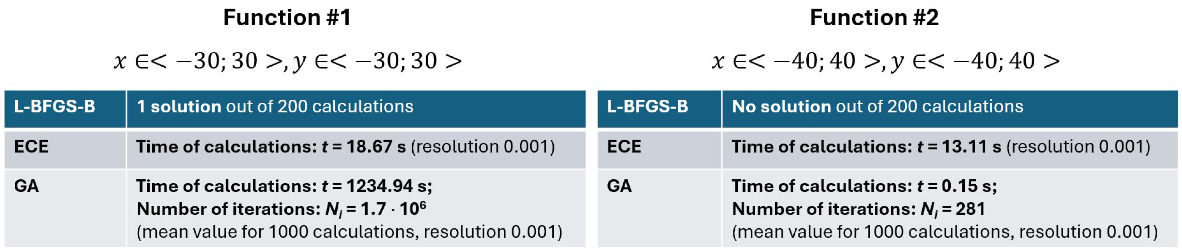
The tests in this task were carried out for test functions #1 and #2 using the largest tested solution domains, i.e., $y\in 〈-30;30〉$ and $x,y\in 〈-40;40〉$, respectively. The results obtained during the tests are presented in Figure 8.

In the case of the L-BFGS-B algorithm, tests showed that this algorithm is not applicable for solving optimization problems defined using either function #1 or function #2. When trying to solve these problems, the algorithm obtained a solution only for function #1, and only in one case out of 200 calculations, in which the starting point of the calculations was randomly selected. In the case of function #2, no result was obtained in analogous conditions. This confirms the features of this algorithm, which is one of the examples of analytical methods based on gradient tracing. Of course, this does not completely exclude the usefulness of the algorithm for use in optimization problems; however, such an algorithm would require adjustments and additional tools (procedures) to enable its effective use.

In the case of the ECE method, the computation time for both functions #1 and #2 was in the order of 10¹ s. The similar calculation times for these functions are related to the resolution of the algorithm’s scanning of the solution domain. On the other hand, small differences in computation time result from the fact that the coordinates of the optimum sought for both functions are slightly different, and the end condition is defined as reaching the value closest to the maximum value (with an assumed permissible difference). Therefore, in cases where the algorithm for each of the functions starts the search from the points $x=x_{min}$ and $y=y_{min}$, the end condition of computation for each will occur after different lengths of time.

The calculation results obtained using the GA method showed that the time taken to reach optimal solutions for problems based on functions #1 and #2 differed significantly. The calculation time for function #1 was in the order of 10³ s and was significantly longer than the time obtained by the ECE method. On the other hand, for function #2, this time was in the order of 10⁻¹ s and was 100 times shorter than that obtained by the ECE method at the same resolution. The results obtained from the comparison of methods did not provide a clear answer to the question of which method has better properties for solving problems differing in the characteristics of the objective function. The universality of the GA method, which showed a very short calculation time for function #2, is, however, very controversial due to the drastically long calculation time obtained for function #1. The reason for this was the use of natural binary encoding, which was discussed earlier. Further research that takes into account the influence of Gray encoding proves that this is the correct explanation for the observed results.

3.3.2. Tests of ECE and GA Methods

The ECE and GA methods, as those that proved to be effective in finding solutions to chosen optimization problems, were subjected to further tests.

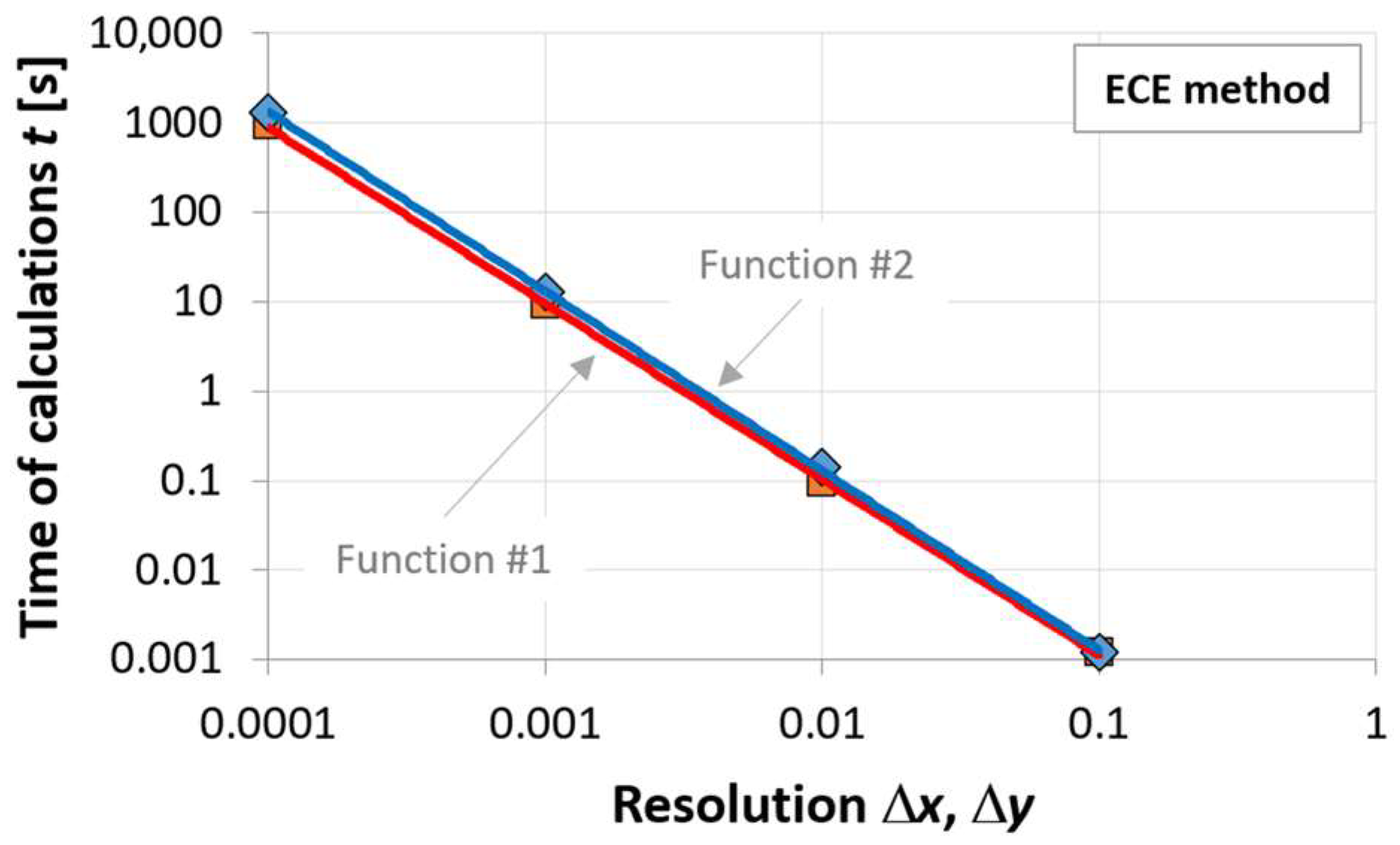
In the case of the ECE method, the influence of the imposed resolution on the computation time was examined. This influence is presented in Figure 9. For both analyzed functions, this time is inversely proportional to the resolution, which is in an intuition-based conclusion.

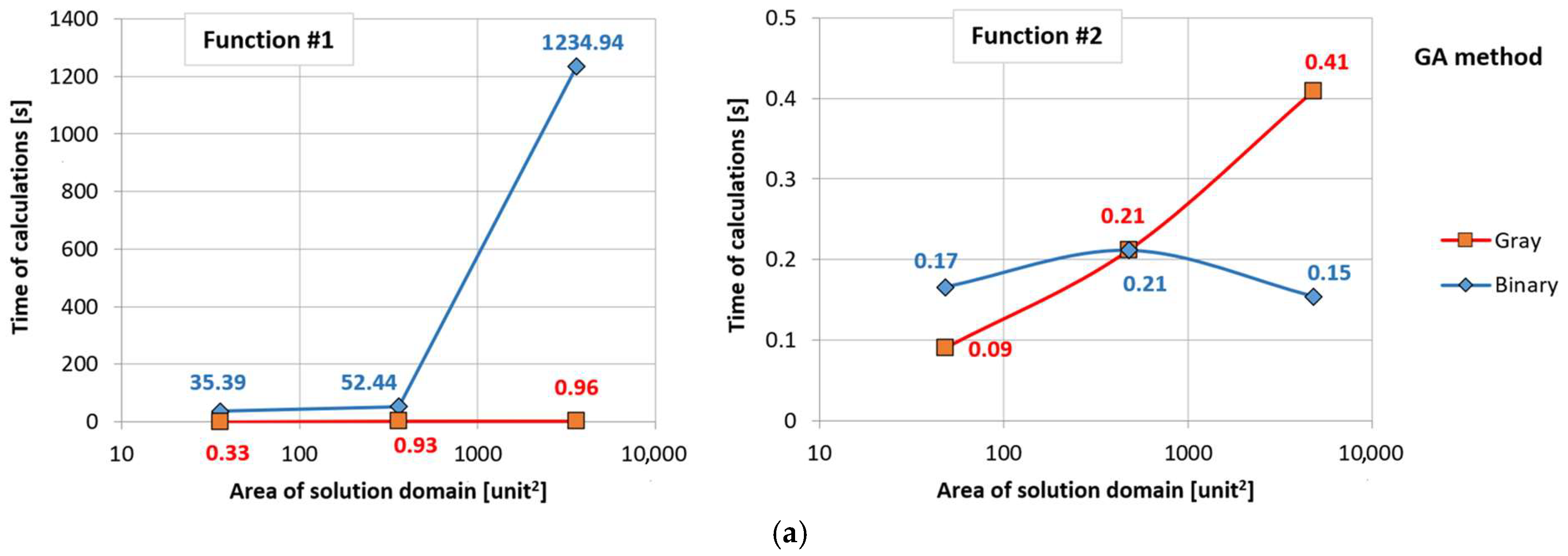
In the case of the GA method, several tests were performed. The first one concerned the influence of the method of encoding the decision variables (natural binary and Gray system). In these tests, calculations were performed for different sizes of the computational domain:

• for function #1 $x,y\in 〈-30;30〉$ and for function #2 $x,y\in 〈-40;40〉$ (maximum analyzed solution area);
• for function #1 $x\in 〈-30;30〉, y\in 〈-3;3〉$ and for function #2 $x\in 〈-40;40〉, y\in 〈-4;4〉$ (area 10 times smaller than the maximum);
• for function #1, $y\in 〈-3;3〉$ and for function #2, $y\in 〈-4;4〉$ (the smallest analyzed area, 100 times smaller than the maximum).

The other parameters of the GA method in these tests remained unchanged (resolution of the solution domain: $∆x=∆y=0.001$; selection method: roulette; probability for the crossover operator $P_c=0.75$; probability for the mutation operator $P_m=0.075$; population size: 10).

The results for both analyzed test functions are presented in Figure 10a.

The results obtained for tests using function #1 clearly indicate significantly better results obtained with Gray encoding—the computation times for this encoding in the analyzed cases did not exceed 1 s, while for natural binary encoding, they ranged from several dozen to several hundred seconds.

In the case of function #2, the obtained results are not so clear. However, for both versions of encoding, the times of obtaining results reached values of less than 0.5 s. Moreover, both relative and absolute differences in these times obtained with natural binary and Gray encoding are much smaller than in the case of results obtained for function #1.

As part of the next test, the influence of both the population size and the choice of the selection method on the computation time was examined. In the case of these tests, the algorithm with Gray encoding was analyzed for the maximum analyzed solution area of the tested functions. The results obtained for the selection carried out following the roulette, tournament, and ranking methods are summarized in Figure 10b.

For tests using function #1 for each of the analyzed selection methods, the trend of decreasing computational time with population growth is maintained. In the case of tests performed for function #2, the differences in the times are not as large. The trends indicate an increase in these times with population growth. In general, for tests using both test functions, significantly shorter times were obtained for obtaining results with the ranking and tournament methods compared to the roulette method.

During the tests of the GA method, the influence of different probability values for the crossover and mutation operators was also checked. These tests showed that the crossover probability value has no significant effect on the computation time (Figure 10c). In this case, the roulette method of selecting individuals also performs worse compared to the ranking and tournament methods.

In the case of the mutation operator, the tests showed that the probability of this operation, which is more than 0.075, significantly shortens the computation time in the case of function #1. For function #2, an opposite trend was observed (Figure 10d). For both test functions, the shortest calculation times were obtained for the ranking and tournament methods, and the longest for the roulette method, regardless of the probability of genetic operators.

3.4. Summary of Tests of Optimization Methods

The tests performed have shown that the analytical method L-BFGS-B and the enumeration method ECE are not effective ways of solving optimization problems in the case of the test functions selected for analysis. In the case of complex objective functions (with numerous local extrema), the L-BFGS-B method makes it impossible to obtain the result. On the other hand, the ECE method, due to the required significant accuracy of results combined with the large size of the solution domain, is characterized by very long computation times, which disqualifies this method in practical applications.

The tests of the GA method have clearly shown that the choice of the coding method in some cases can have a very significant impact on the computation time. Based on the tests performed, it is recommended to use Gray encoding instead of natural binary encoding. In general, even though some of the tests performed did not provide unambiguous results, it should be recognized that the best results (with the shortest computation times) can be obtained with:

• choosing the tournament or ranking method as the selection method;
• using high values of the crossover probability;
• selecting large population sizes of individuals;

Other parameters, such as the probability of mutation, should be selected depending on the characteristic of the problem being optimized.

The considerations so far concern the optimization of the adopted algorithm in terms of the computation time. The end condition of the calculations was to achieve the global maximum with the assumed accuracy, as the global maximum was known for the test functions. In practical applications, such as the optimization of the operation of units installed in the hydropower plant, which is the subject of further consideration, the optimum solution is not known. In such cases, the possible end condition of calculations may be:

• performing a specified number of iterations;
• exceeding the specified computational time;
• no changes in the value of the adaptation function in subsequent iterations.

These conditions should be selected depending on the characteristics of the optimization problem.

4. Sustainable Hydropower Plant Operation

The mathematical model used in this paper, including the decision variables, objective function, and constraints, is outlined in this chapter, where all the specific equations used for the defined problem are presented.

4.1. Formulation of the Optimization Problem

The next stage of this work, consisting of recognizing the properties of optimization methods in terms of their usefulness in the sustainable operation of hydropower plants, was to solve an example task for optimizing a hydropower plant equipped with three units. The goal of the optimization was to determine the operating points of all hydro units (flow through each of the hydro units $Q_{u\_i}$ at a given constant head value $H=const.$) depending on the given flow through the power plant ($Q_{hpp}$). The criterion for this optimization was to maximize the efficiency of the power plant under the given conditions: ${\eta }_{hpp}{\left(Q_{hpp}\right)}_{H=const}\to max$. It was assumed that the hydro units are identical in terms of the relationship between the efficiency and the flow rate through each hydro unit ${\eta }_{u\_i}\left(Q_{u\_i}\right)={\eta }_u\left(Q_{u\_i}\right)$. The objective function for this task is defined as follows:

$${\eta }_{hpp}{\left(Q_{hpp}\right)}_{H=const}={\displaystyle \frac{{\sum }_{i=1}^3\left[{{\eta }_u\left(Q_{u\_i}\right)·Q}_{u\_i}\right]}{{\sum }_{i=1}^3{Q}_{u\_i}}}\to max$$

(4)

The decision variables in this problem are the flow rate values through each hydro unit $Q_{u\_i}$ for $i=1\dots 3$. The input data of the optimization problem are a set of constraints formulated as follows:

• The flow through the hydropower plant $Q_{hpp}$ is in the range of 75 m³/s to 540 m³/s and is equal to the sum of the flows through all hydro units:

  $$Q_{hpp}={\sum }_{i=1}^3{Q}_{u\_i} ; 75 {\mathrm{m}}^3/\mathrm{s}\le Q_{hpp}\le 540 {\mathrm{m}}^3/\mathrm{s}$$

  (5)
• The flow through each of the hydro units $Q_{u\_i}$ can take the value 0 m³/s or a value from a range of $Q_{min}=$ 75 m³/s to $Q_{max}=$ 180 m³/s, i.e.,

  $$Q_{u\_i}=0 {\mathrm{m}}^3/\mathrm{s} ⌵ 75 {\mathrm{m}}^3/\mathrm{s}\le Q_{u\_i}\le 180 {\mathrm{m}}^3/\mathrm{s}$$

  (6)

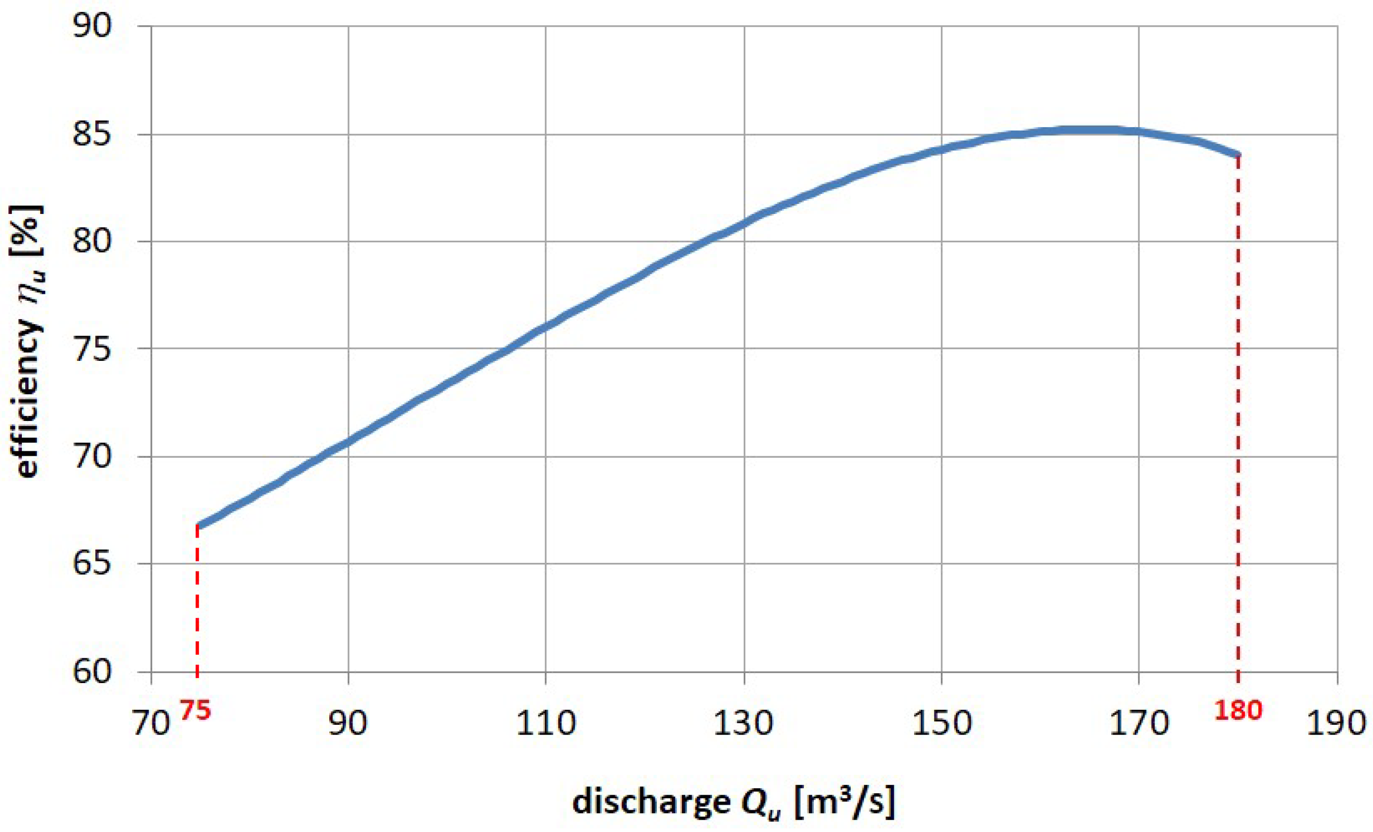
The efficiency function of the hydro units in relation to the flow ${\eta }_u\left(Q_u\right)$ is shown in Figure 11.

It is assumed that the function in Figure 11 is described by the following fourth-degree polynomial:

$${\eta }_u\left(Q_{u\_i}\right)=A·Q_{u\_i}^4+B·Q_{u\_i}^3+C·Q_{u\_i}^2+D{·Q}_{u\_i}+E$$

(7)

where: A = −0.0000000764

B = +0.0000176463

C = −0.0008605875

D = +0.2157098756

E = +50.4182036066

The problem described by Equations (4)–(7) was used to test the computational algorithm prepared for the optimization of the hydropower plant operation. The algorithm was based on the GA method, which, due to the results obtained at the testing stage, was selected as the target tool for its solution. The following tests consisted of calculating water flows through hydro units for total flows through hydropower plant $Q_{hpp}$, changing from minimum to maximum values with a step of 10 m³/s. The results of the calculations using the GA method were compared to the results obtained using the ECE method, which is very expensive but always provides the correct solution.

4.2. Results Obtained Using the ECE Method

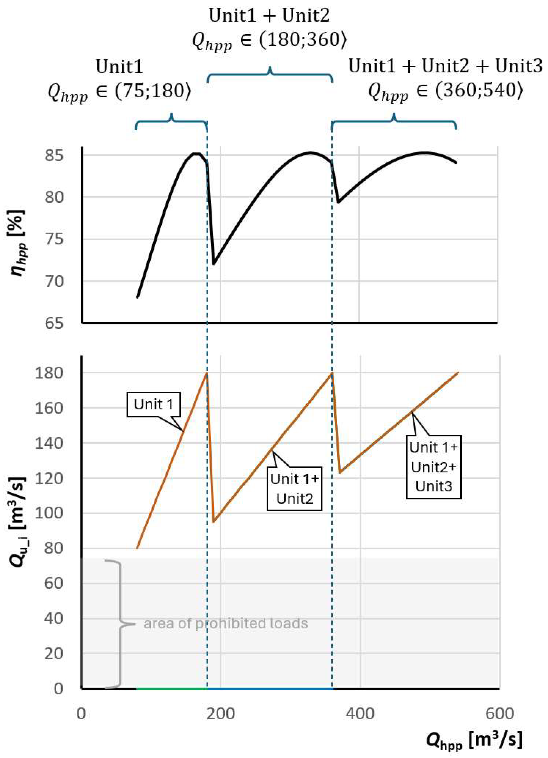
In a situation where a hydropower plant is equipped with identical units, an equal distribution of flows through them seems to be optimal as it follows intuition. Such a solution is presented in Figure 12. However, the results obtained using the ECE method presented in Figure 13 showed that the flows through each hydro unit in the case of an optimum distribution of total flow differ from each other:

• when two hydro units are in operation for flows through the power plant: $180 {\mathrm{m}}^3/\mathrm{s}<Q_{hpp}<260 {\mathrm{m}}^3/\mathrm{s}$;
• when three hydro units are in operation for flows through the power plant: $360 {\mathrm{m}}^3/\mathrm{s}<Q_{hpp}<410 {\mathrm{m}}^3/\mathrm{s}$.

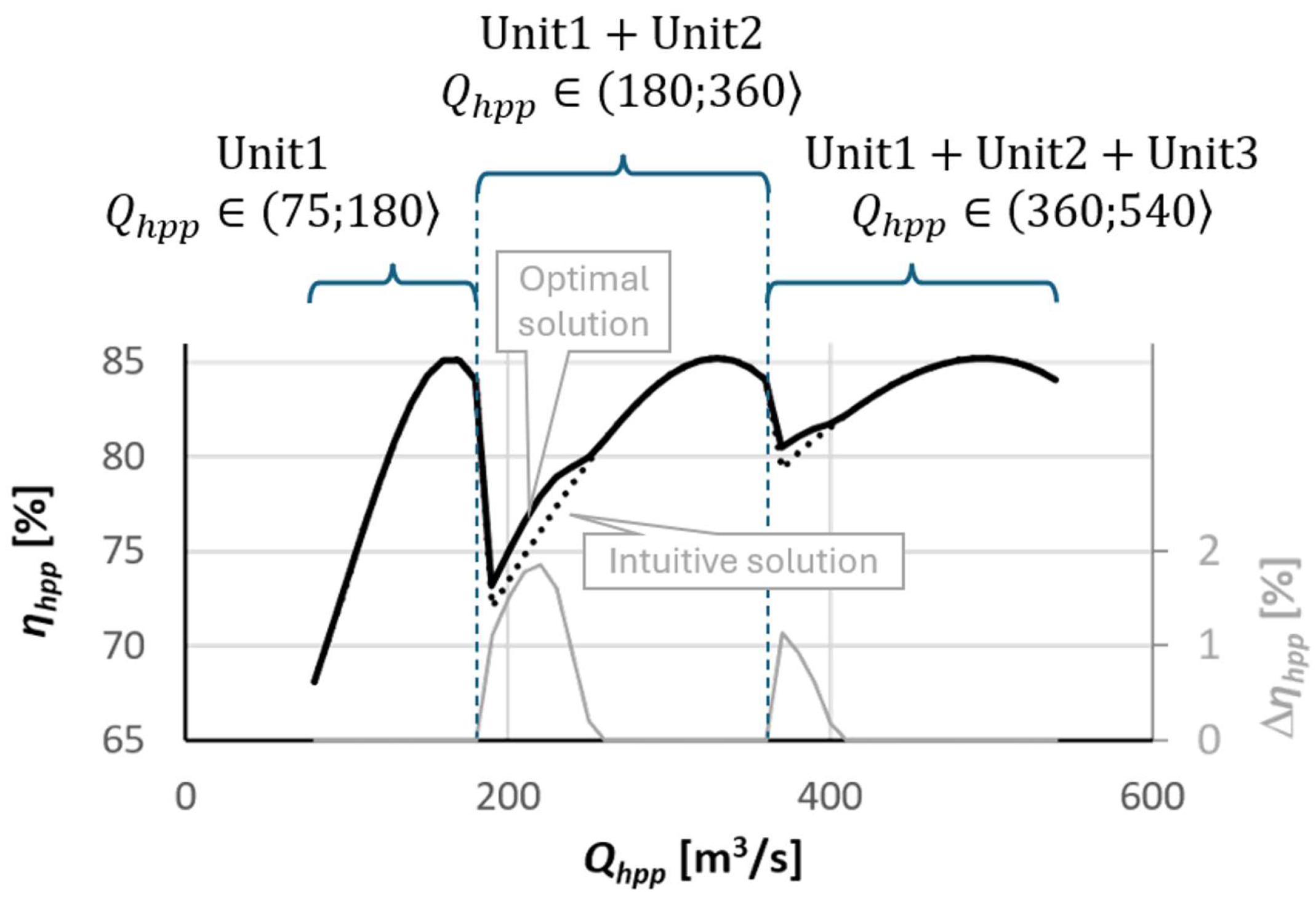
The differences between the results obtained using the optimization algorithm and the intuitive results are presented in Figure 14. The optimal results for the analyzed problem allow for obtaining a power plant efficiency of up to approx. 2% higher than in the case of an equal distribution of water flow between the hydro units in operation.

4.3. Results Obtained Using the GA Method

When using the GA algorithm to solve the optimization problem of the operation of a power plant equipped with three identical hydro units, the experience gained during the algorithm testing stage using test functions was used. Consequently, the tournament method was used as the selection method, while the crossover and mutation probabilities were assumed to be equal to 0.75 and 0.075, respectively. Gray scheme encoding was used to encode decision variables. The basic difference between the algorithm testing phase based on test functions #1 and #2 and the power plant optimization problem is the form of the solution domain. According to Equation (6), the flow through the hydro units can take the value of zero or values between 75 m³/s and 180 m³/s. Therefore, an appropriate effective solution was required to reject solutions in which the hydro unit flows are outside of this area. This is reflected in the construction of individuals that contain information about each of the hydro units of the power plant.

4.3.1. Construction of Individuals

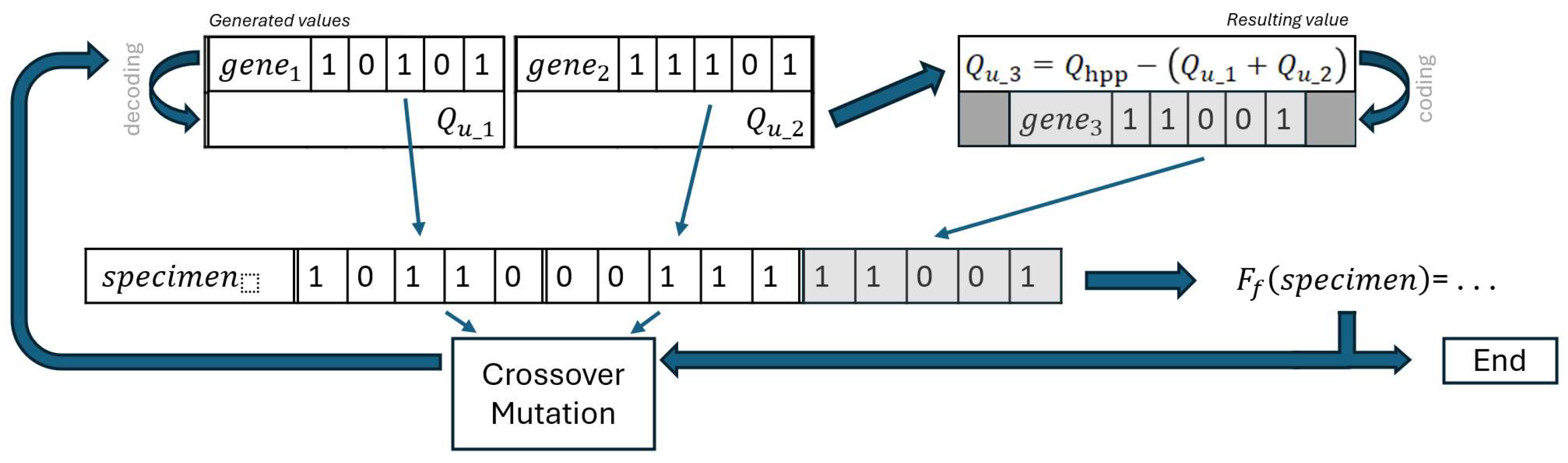
The use of the GA method consists of generating an individual (specimen) that will be characterized by the highest value of the fitness function $F_f$, defined as follows:

$$F_f\left(specimen\right)={\displaystyle \frac{{\sum }_{i=1}^3\eta \left(Q\left({gene}_i\right)\right)·Q\left({gene}_i\right)}{{\sum }_{i=1}^{3}Q\left({gene}_i\right)}}$$

(8)

In Equation (8), ${gene}_i$ is the encoded form of the decision variables $Q_{u\_i}$ presented in Equation (4)—$Q_{u\_i}=Q\left({gene}_i\right)$ for the $i$-th hydro unit. In turn, the efficiency of the $i$-th hydro unit is as follows—${\eta \left(Q\left({gene}_i\right)\right)=\eta }_{u\_i}={\eta }_u$. The encoding scheme is shown in Figure 15. The genes reflecting the decision variables were subjected to the genetic operators, i.e., crossover and mutation procedures. In the applied approach, the last of the genes was not subjected to genetic operators and the decision variable it represents (the flow through the third hydro unit) is the resulting value of the difference in the flow through the power plant and the sum of the flows through the remaining two hydro units.

4.3.2. Penalty Function

Such a solution for coding an individual in the GA method automatically ensured that the condition given by Equation (5) ($Q_{hpp}={\sum }_{i=1}^3{Q}_{u\_i}$) is met. For the remaining conditions presented in Equation (6), concerning flows through each of the hydro units, the application of appropriately defined penalties is required. The values of these penalties are intended to reduce the value of the fitness function of a given individual constructed from the generated genes in cases where the genes that make up its structure come from a prohibited solution area, i.e., from outside the area defined by Equation (6).

Reducing the value of the fitness function $F_f$ is intended to direct the calculations to obtain solutions from the permitted solution area. The use of a penalty function is one of several solutions that make achieving such a goal possible. The values of these penalties are defined as a function that assumes higher values the further the decision variable represented by a given gene is from the area of the permitted solution. The penalty assigned to an individual is defined as the largest penalty imposed on the genes from which it is constructed.

$$F_{penalty}\left(specimen\right)=\max \left(F_{penalty}\left({gene}_i\right)\right)$$

(9)

The general form of the penalty function for the analyzed individual consisting of three genes can be written as:

$$F_{penalty}\left({gene}_i\right)=F_f\left(specimen\right)·F_s\left({gene}_i\right)$$

(10)

where $F_s\left({gene}_i\right)$ is a function taking values from 0 to 1.

In the case of the first two genes (${gene}_1$ and ${gene}_2$ subjected to genetic operators), the prohibited area of operation is $Q_{u\_i}\in (0,Q_{\mathrm{m}\mathrm{i}\mathrm{n} \_u_i})$, where $Q_{u\_i}$ is the flow rate value corresponding to the $i$-th gene (${gene}_i$), while $Q_{\mathrm{m}\mathrm{i}\mathrm{n} \_u_i}$ denotes the minimum flow rate value permissible for a given hydro unit during its operation (according to Equation (6)). 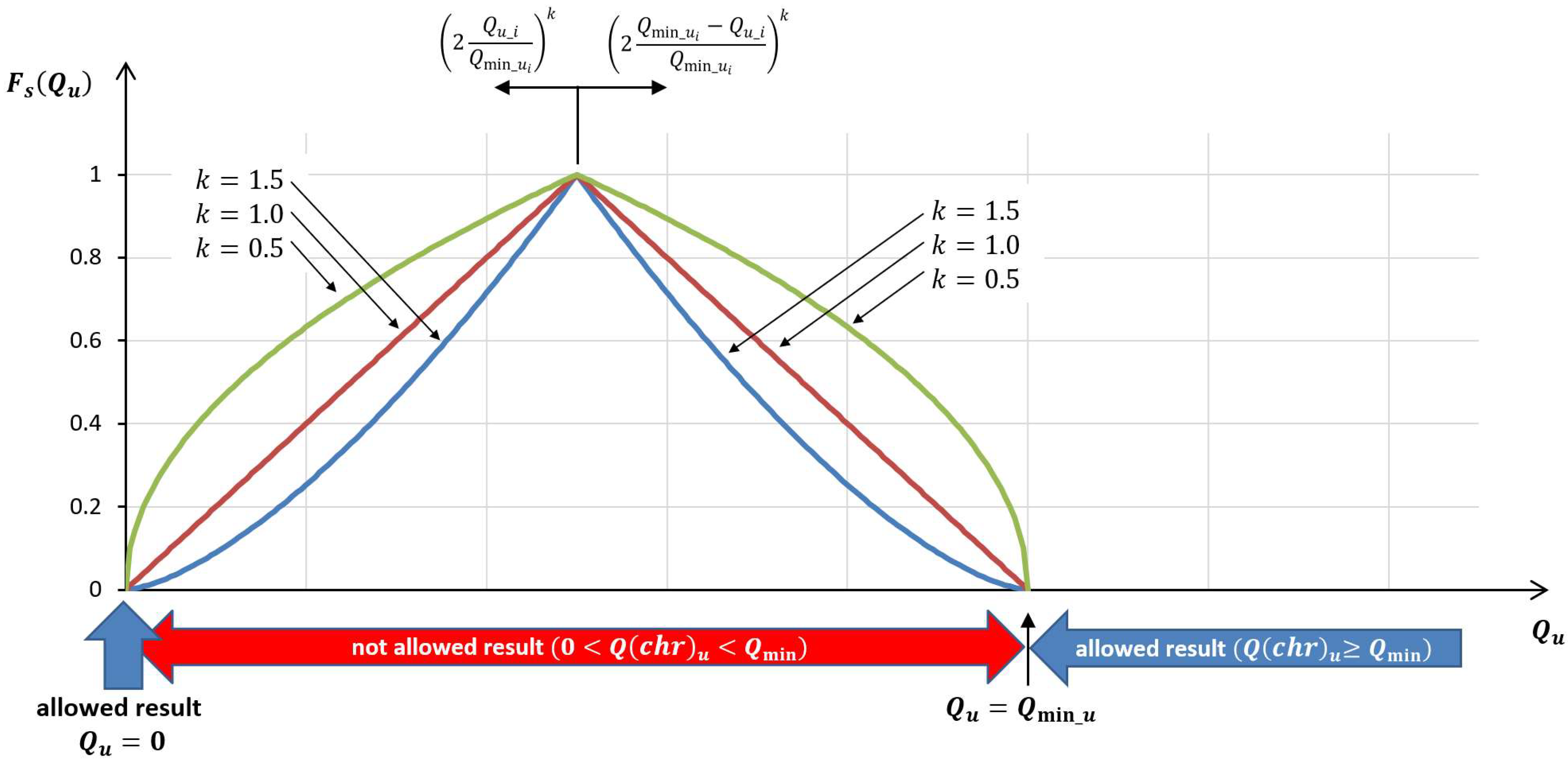The $F_s\left({gene}_i\right)$ function is calculated according to the following formula:

$$Q_{u\_i}\in \left(0,Q_{\mathrm{m}\mathrm{i}\mathrm{n} \_u_i}/2\right) \to F_s\left({gene}_i\right)={\left(2{\displaystyle \frac{Q_{u\_i}}{Q_{\mathrm{m}\mathrm{i}\mathrm{n} \_u_i}}}\right)}^k$$

(11)

$$Q_{u\_i}\in \left(Q_{\mathrm{m}\mathrm{i}\mathrm{n} \_u_i}/2,Q_{\mathrm{m}\mathrm{i}\mathrm{n} \_u_i}\right) \to F_s\left({gene}_i\right)={\left(2{\displaystyle \frac{Q_{\mathrm{m}\mathrm{i}\mathrm{n} \_u_i}-Q_{u\_i}}{Q_{\mathrm{m}\mathrm{i}\mathrm{n} \_u_i}}}\right)}^k$$

(12)

An important issue is the influence of the exponent $k$ on the values of the penalty function. The dependence of the shape of the $F_s$ function on the exponent $k$ is shown in Figure 16.

For gene no. 3, representing the flow through hydro unit #3, the $F_s$ function is additionally defined for flows smaller than 0 m³/s and greater than the $Q_{\mathrm{m}\mathrm{a}\mathrm{x} \_u_3}$ defined for the third hydro unit. Its shape is analogous to those shown in Figure 16 (the value of the $F_s$ function in the above ranges increases with the decrease of $Q_{u\_3}$ below 0 and with the increase of $Q_{u\_3}$ above $Q_{\mathrm{m}\mathrm{a}\mathrm{x} \_u_3}$). Therefore, for describing the values of the $F_s$ function of the third hydro unit, Equations (11) and (12) apply, while in the range of flows below 0 m³/s and greater than $Q_{\mathrm{m}\mathrm{a}\mathrm{x} \_u_3}$, the equations presented below are used:

$$Q_{u\_3}\in \left(-{\sum }_{i=1}^2{Q}_{\mathrm{m}\mathrm{a}\mathrm{x} \_u_i} ;0\right) \to F_s\left({gene}_3\right)={\left({\displaystyle \frac{Q_{u\_3}}{{\sum }_{i=1}^2{Q}_{\mathrm{m}\mathrm{a}\mathrm{x} \_u_i}}}\right)}^k$$

(13)

$$Q_{u\_3}\in \left(Q_{\mathrm{m}\mathrm{a}\mathrm{x} \_u_3}; {\sum }_{i=1}^3{Q}_{\mathrm{m}\mathrm{a}\mathrm{x} \_u_i}\right) \to F_s\left({gene}_3\right)={\left({\displaystyle \frac{Q_{u\_3}-Q_{\mathrm{m}\mathrm{a}\mathrm{x} \_u_3}}{{\sum }_{i=1}^3{Q}_{\mathrm{m}\mathrm{a}\mathrm{x} \_u_i}-Q_{\mathrm{m}\mathrm{a}\mathrm{x} \_u_3}}}\right)}^k$$

(14)

The value of the fitness function after imposing the penalties defined in the method presented in Equations (11)–(14) is given as follows:

$${F_f}^{*}=F_f-F_{penalty}$$

(15)

When using the approach based on Equation (9), the value of the fitness function ${F_f}^{*}$ after imposing the most unfavorable penalty (for $\max \left(F_{penalty}\left({gene}_i\right)\right)$, i.e., for $F_s\left({gene}_i\right)=1$), can reach a minimum value of 0.

4.3.3. Results and Further Modifications of the GA

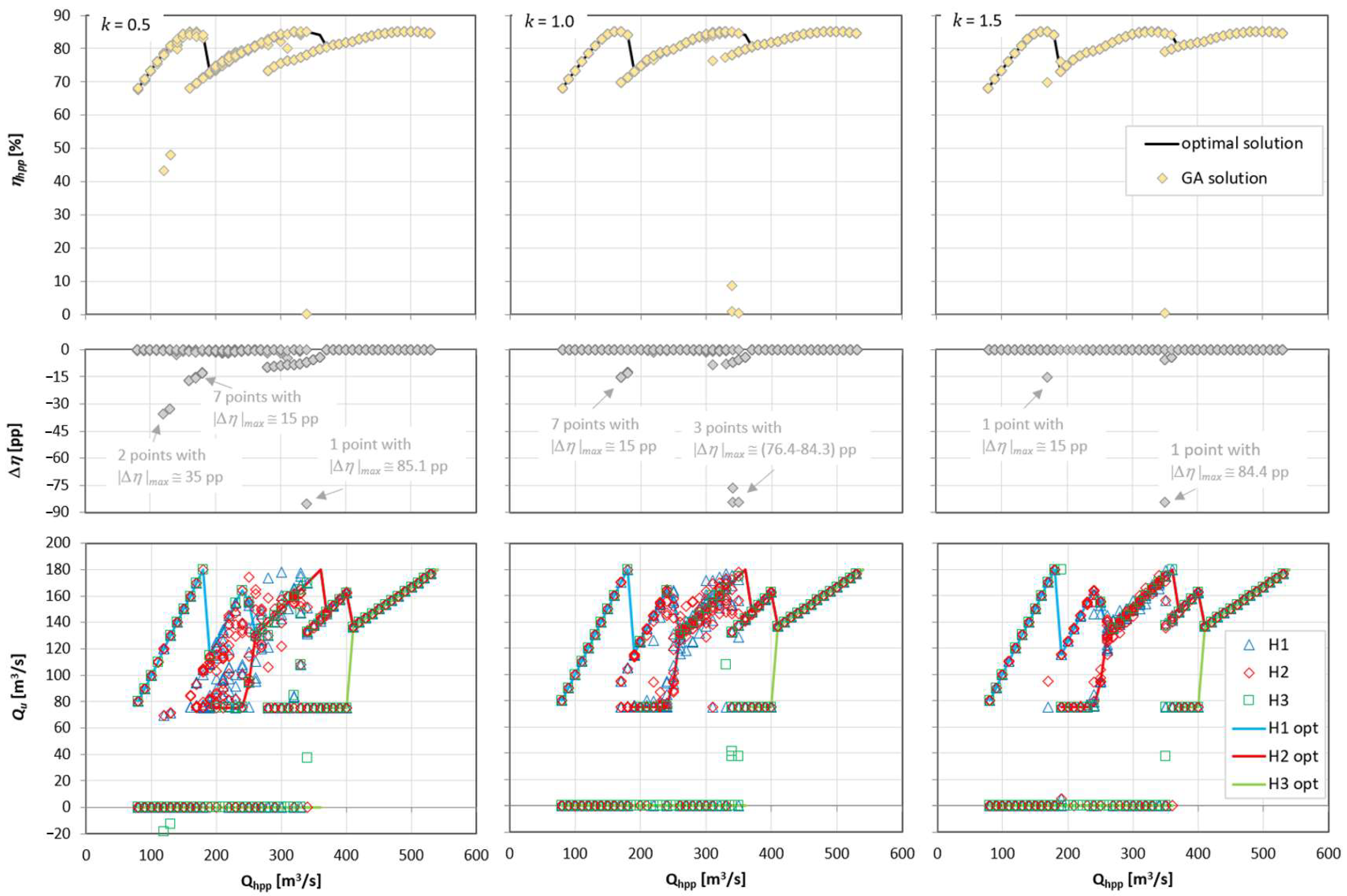
The exponent $k$ in the penalty function has a direct impact on the quality of calculations performed using the GA. As part of the work, several tests were conducted to observe the effect of this parameter on the obtained results.

The results for the exponent $k$ in Equations (11)–(14) equal to 0.5, 1, and 1.5 are presented in Figure 17. Calculations using the GA method consisted of determining the optimal flows through each of three hydro units for a given total flow through the power plant. The flows through the power plant were set from the minimum to the maximum value in steps of 10 m³/s. At each of these points, the calculations were performed 10 times, performing 1000 iterations in each of these calculations. The results are presented in the form of:

• the efficiency of the power plant ${\eta }_{hpp}\left(Q_{hpp}\right)$ determined for a constant head ($H=const.$) using Equation (4)—the optimal solutions obtained using the ECE method (${\eta }_{hpp\_opt}$—continuous line) is overlaid with solutions obtained using the GA algorithm (${\eta }_{hpp\_GA}$—points);
• the difference between the efficiency of the power plant for the optimal solution (${\eta }_{hpp\_opt}$) and the efficiency calculated using the GA method (${\eta }_{hpp\_GA}$):

  $$∆\eta ={\eta }_{hpp\_opt}-{\eta }_{hpp\_GA} \left[\mathrm{p}\mathrm{p}\right]$$

  (16)
• flows through each of the hydro units $Q_{u\_i}\left(Q_{hpp}\right)$ determined using the GA method (points), superimposed on the results of the optimal flow distribution determined using the ECE method (line).

As can be seen from the results presented in Figure 17, the use of a constant value of the $k$ exponent to define the penalty functions does not provide an optimal solution in all operation points in the problem under investigation. Many of the hydro unit operating points determined by the GA do not meet the conditions imposed by the constraints (Equations (5) and (6)). This causes the adaptation function for these points to significantly deviate from the optimal solution; at these points, its value is lower by several to almost 90 pp than the corresponding efficiency for the optimal solution. Such a large difference means that the result obtained using the GA is at the place of the maximum possible penalty, i.e., for $F_s\cong 1$. However, it can be observed that in the case of using a larger value of the exponent $k$, the obtained results are slightly better than for the other analyzed cases.

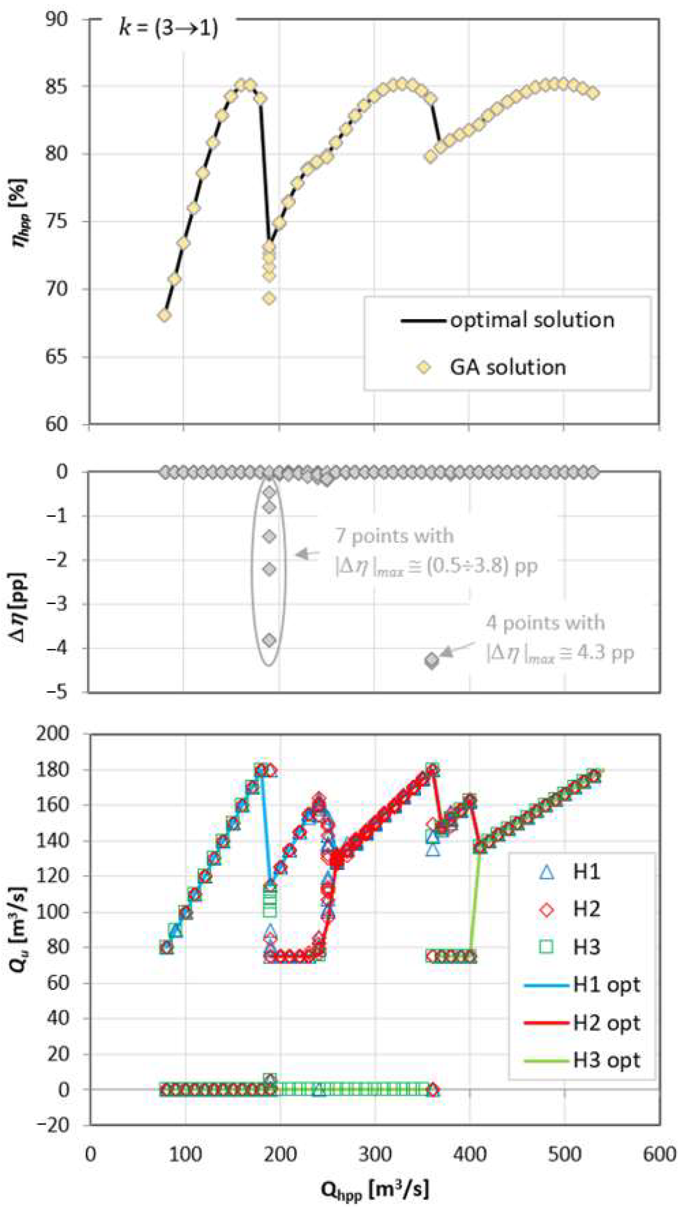
The results obtained for constant values of the $k$ exponent were considered unsatisfactory due to significant deviations from the optimal solution. This assessment was particularly influenced by the fact that the solutions contained operating points in prohibited areas, in particular at the beginning of the area where the calculation results indicated the need to operate all three hydro units (for $Q_{hpp}$ = (350–360) m³/s). Therefore, a new approach was proposed consisting of differentiating the value of the exponent $k$ depending on the distance of the obtained result (individual) from the area of permissible solutions. Many configurations of the variable value of the exponent $k$ were tested. Ultimately, the best solutions were obtained assuming that the value of $k$ is higher near the permitted area and decreases the further the result is from this area. 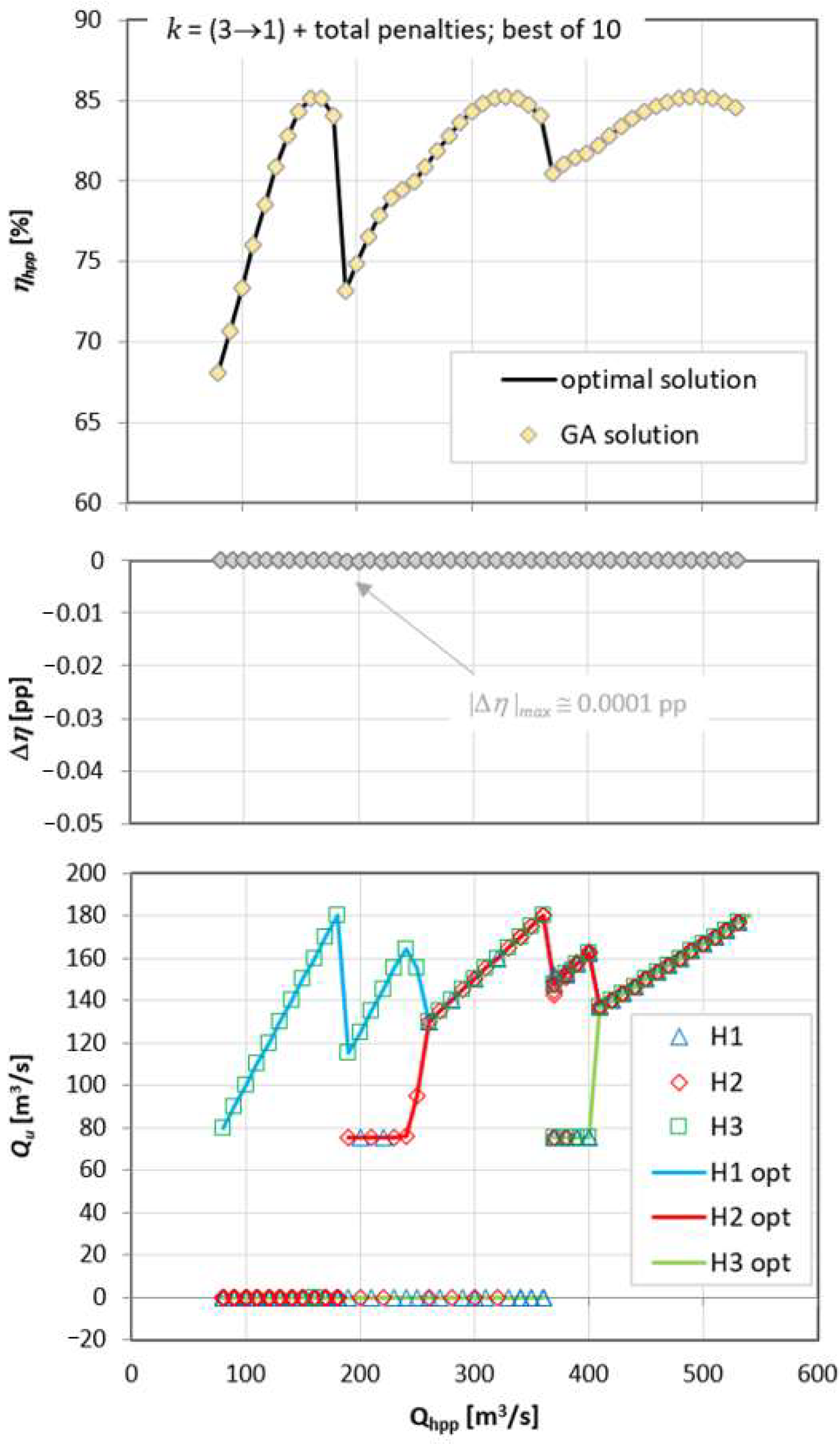An example of calculations for the $k$ exponent varying from 3 to 1 is presented in Figure 18. A significant improvement in the quality of the obtained results is noticeable. Only for flows requiring the operation of two hydro units ($Q_{hpp}$ = 190 m³/s) were single results in the prohibited solution area found, i.e., with a flow through the hydro unit slightly greater than 0 m³/s or in the area between 75 m³/s and 110 m³/s. In addition, the GA algorithm generated only a few results that deviated by more than 1 pp from the optimal results—the maximum discrepancy from the optimal solution was 4.3 pp and it was found for $Q_{hpp}$ = 360 m³/s. Among the remaining results, several calculated operating points of the hydro units were characterized by efficiency that deviated from the optimal efficiency by less than 1 pp.

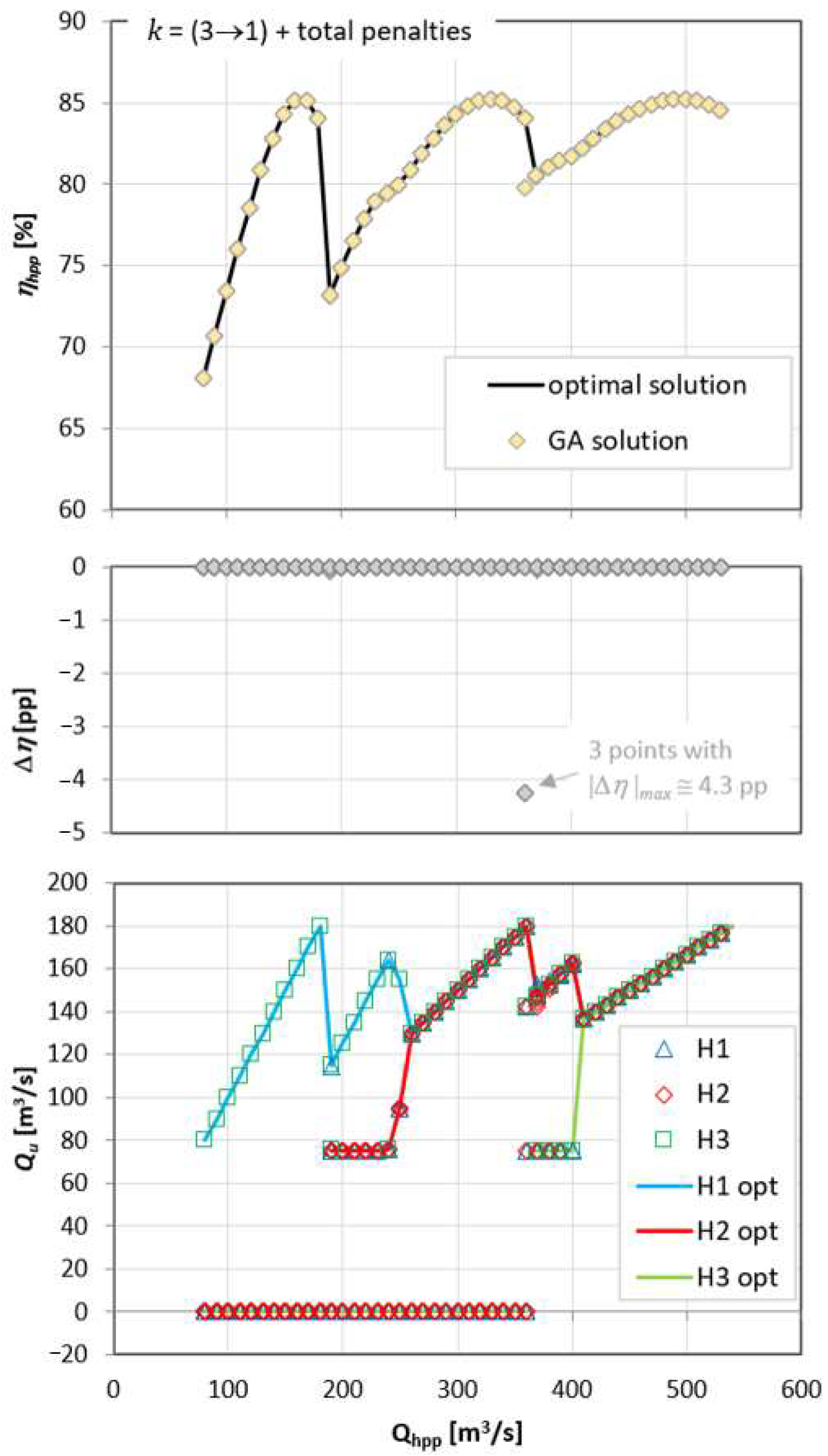
The analysis of the aforementioned violations of the prohibited area ($Q_{hpp}$ = 190 m³/s) showed that the reason for generating such results was that the value of penalties for minor exceedances was too low, even in a situation when it concerned more than one hydro unit. In response to this problem, it was proposed to increase the penalty for individuals composed of genes from the prohibited range of flow by adding up the penalty values. This means that Equation (9) was replaced with the following:

$$F_{penalty}\left(specimen\right)={\sum }_{i=1}^3{F}_{penalty}\left({gene}_i\right)$$

(17)

The application of such a modified procedure allowed the results presented in Figure 19 to be obtained. As shown, a significant improvement was obtained in the operation of two hydro units compared to the results obtained based on Equation (9). No improvement was found at point $Q_{hpp}$ = 360 m³/s, which should not be surprising as at this point, the divergence from the optimum solution does not result from determining the flow through any hydro unit located outside the permitted area. Therefore, the modification introduced in Equation (17) could not have affected the calculation results at this point of the power plant flow.

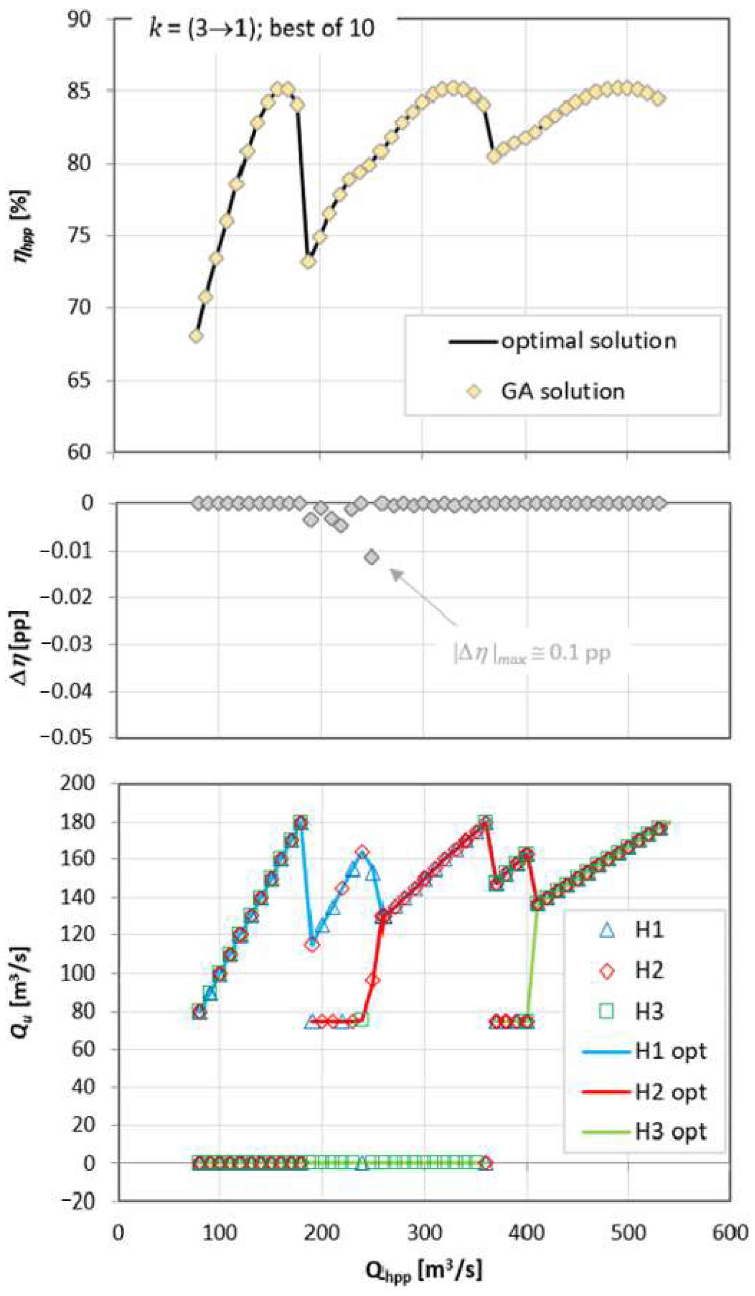
It should be noted that for the 10 calculations performed for each given power plant flow, the GA algorithm always produced at least one solution that was optimal or very close to the optimal. Taking advantage of this fact, only results with the highest power plant efficiency were selected from the calculation results. The results obtained using Equation (9) and Equation (17) are presented in Figure 20 and Figure 21, respectively. The discrepancy between the calculation results using th GA and the optimal results in the first case does not exceed 0.1 pp and was only 10⁻³ pp for the second case. These results indicate the correctness of the proposed approach.

It should be noted that the proposed approach, which involves carrying out calculations several times and then selecting the results for maximum efficiency, generates computational costs that are several times higher. In the analyzed cases, the time required to perform calculations is approx. 0.4 s when using:

• a population of 40 individuals
• Gray system encoding
• 10³ calculation iterations
• ranking method selection

This means that generating one calculation point shown in Figure 20 and Figure 21 required approx. 4 s. It should be emphasized that this time is strongly dependent on the parameters presented above, and also on:

• the number of hydro units and their availability (readiness for operation),
• the complexity of the analyzed issue, e.g.,

  ○

  equipping the water barrage at which the power plant is installed with a weir to allow water flows that are too low for energy use;

  ○

  equipping the water barrage at which the power plant is installed with a lock, prioritizing supply flows to allow river transport,

  ○

  significant variability of the power plant head, which determines the variability of hydro unit characteristics.

Therefore, it can be assumed that in some very complicated cases, the strategy of multiple calculations may not be sufficiently beneficial to achieve sustainability in using the available water resources. However, it is worth mentioning that the calculations produced by the enumeration method (for the analogous resolution of results, as presented in Figure 20 and Figure 21) require a time that is approximately four times longer than in the case of the GA. It is expected that the degree of complexity of the problem may also significantly increase these differences.

In the case of more complicated cases, it is justified to continue searching for solutions that allow for reducing these costs by developing other procedures within the use of the GA method, i.e.,

• improving the method based on penalty functions;
• further work on matching the parameters of genetic operators (crossovers, mutations);
• using different population sizes, numbers of iterations, or different end conditions of calculations.

A very promising direction in the development of methods to solve optimization problems encountered in practice is the use of different optimization methods at different stages of calculations, i.e., hybrid methods. This would allow taking advantage of the methods used in such an approach to obtain reliable and repeatable calculation results.

5. Summary and Conclusions

The results of the work presented in this paper confirmed the commonly known features of optimization methods and enabled their quantitative assessment in the context of their application in engineering practice. Tests were conducted on methods selected from three basic groups, i.e., analytical, enumeration, and randomized methods, with the latter showing a significant advantage. This work showed that the GA method, which was chosen as a representative randomized method, is significantly better in terms of the time taken to obtain a solution and the relatively low computing power requirements. These features of the GA method make it an effective tool for solving various optimization problems. However, the conditions for achieving this goal are:

• correct formulation of the optimization problem together with an appropriate definition of constraints imposed on the decision variables,
• appropriate selection of implementation and main parameters of basic procedures that are characteristic of this method, i.e.,

  ▪

  encoding systems,

  ▪

  selection procedures,

  ▪

  genetic operators.

• appropriate selection of the population size and the definition of the end condition of the calculations,
• development of methods for effectively eliminating the results of calculations from the prohibited area of solutions, e.g., through appropriately defined penalty functions.

This work has shown that the above-mentioned aspects significantly affect the quality of the obtained results. Only the fulfillment of all of these conditions, taking into account the characteristics of a given problem, guarantees achieving correct results and ensuring the sustainable use of water as a natural energy resource at an acceptable calculation cost and efficiency.

The features of the GA method have proven to be very useful in issues related to load distribution between units installed in hydropower plants, which was the main element of the presented work. The calculation examples have proven that the intuitive way of operating hydropower plants may significantly differ from the optimal way in terms of using the available hydropower potential. This is an extremely valuable observation that could potentially be of great importance not only for increasing the profitability of operating hydropower plants but above all for ensuring the sustainable use of water resources.

The procedures used for calculations by the GA method have indicated potential directions for their improvement. The method based on the penalty function with the proposed modifications, although it allowed satisfactory results to be obtained in the tests presented, may be insufficient for cases with a higher degree of complexity, especially in terms of the calculation cost–quality relationship. When using the GA method, we should be aware of some limitations of this method, which result from the need to proceed with caution in the case of very complicated problems, especially those involving numerous areas of prohibited solutions. As shown in this paper, preparing appropriate procedures to exclude results from these areas can be troublesome, if not impossible. Therefore, further work on the GA method is planned. The main goal will be to search for solutions that allow for better adjustment of algorithm parameters to the characteristics of problems related to the optimal operation of multi-unit hydropower plants. Taking into account the remaining constraints resulting from the obligation to share water resources with all other users, concerning, above all, the needs of the natural environment and hydrology, will be a further step towards achieving balanced and environmentally compatible water management. Optimization problems requiring numerous constraints can be introduced into the genetic algorithm in a relatively user-friendly way. A rather attractive solution allowing for significant progress in this area may be the combination of this method with other methods in order to make the best use of their features in obtaining a certain solution to the problems of optimal load distribution of units in hydroelectric power plants. That is why it is expected it will be possible to create an effective tool for the optimal use of water resources in the systems in which the hydroelectric facilities are located.

The importance of increasing the efficiency of a hydroelectric power plant by optimizing the load distribution to individual hydroelectric units can be demonstrated by the example of the Włocławek power plant, the largest run-of-river hydroelectric power plant in Poland. The introduction of an optimization algorithm to its operation allowed for an increase in its efficiency (increased production) by approx. 1.5%. This means that the production and profitability of the power plant increased measurably by this amount, as well as the use of available potential, without harming the natural environment and maintaining its sustainable management [28].

Since optimal use of natural resources is an element of sustainable development, such a tool will also help us to meet the needs of the present generation without reducing the chances of future generations meeting theirs.