Abstract
This study focuses on identifying suitable areas for the installation of water-pumping windmills in Thailand, which require wind speeds of at least 4 m/s to operate efficiently. A simple combined approach is introduced, integrating the Entropy–TOPSIS method complete linkage clustering to prioritize and categorize potential locations. Out of 271 initial areas, 28 have been selected based on their ability to meet the 4 m/s wind speed threshold. The Entropy–TOPSIS method first evaluates these areas based on monthly wind speed and agricultural area. The analysis reveals that regions with higher wind speeds generally score better for wind energy potential, while areas with larger agricultural spaces tend to score higher for farming suitability. The final integrated scores show that agricultural area is more significant, with a weight of 0.7788, compared to the wind speed weight of 0.2212. The areas are then ranked, and complete linkage clustering groups them into six categories, from the most to the least suitable for windmill installation. A sensitivity analysis confirms the robustness of the clustering method, as the group composition remains stable despite minor changes in weight adjustments. This approach simplifies decision-making for sustainable energy investments in Thailand agriculture sector.
1. Introduction
Thailand is well-known as a leading global agricultural producer, with almost 30% of its workforce engaged in the agricultural sector [1]. The country’s varied topography allows it to cultivate over 13 economic crops, exporting their products worldwide. Agriculture plays a crucial role in Thailand’s national income. However, Thai farmers face challenges such as low annual incomes and significant debt, largely due to high production costs, particularly the energy expenses associated with water-pumping systems. To manage these costs, many Thai farmers have traditionally replaced electric or gasoline/diesel water pumps with wind-powered water-pumping windmills. These windmills are usually 9 to 15 m tall, can operate efficiently at low wind speeds, starting from a cut-in speed of 2 m/s, and can provide water without incurring electricity or fuel costs. According to the Department of Alternative Energy Development and Efficiency (DEDE) [2], the average wind speed in Thailand ranges from approximately 3 to 5 m/s, which is classified as low to moderate. The southern regions of Thailand experience higher average wind speeds compared to other parts of the country. According to data from the Thailand Office of Agriculture Economics [3] and the Thailand Land Development Department [4], nearly 54% of the land in the western region of Southern Thailand is highly suitable for agriculture and five out of six provinces in this region are recognized for their high-quality agricultural production. This indicates strong potential for wind energy investment in these areas. Various researchers [5,6,7,8] evaluated wind potential in agricultural areas by collecting and analyzing wind data with precise instruments and mathematical methods. However, these methods are impractical for Thai farmers due to the lack of access to such instruments and budget constraints. Based on previous studies, it is recommended to prioritize wind quality in the western regions of Southern Thailand using monthly wind data and other agricultural data from secondary sources. Sakon et al. [9,10] utilized either the Analytical Hierarchy Process (AHP) or the complete linkage clustering method with secondary wind data. AHP successfully ranked areas based on wind energy potential, while the complete linkage clustering method categorized areas with similar wind quality. However, these methods were complex to apply to the wind dataset. Simpler approaches, such as the entropy weight method and Technique for Order Preference by Similarity to Ideal Solution (TOPSIS), have been explored for prioritizing alternatives based on final scores, aiding in rational decision-making. For instance, Jingwen [11] used a combination of entropy weight and TOPSIS to select an appropriate Management Information System (MIS) based on five purchasing criteria. Similarly, Xiangxin et al. [12] applied the entropy weight method to safety conditions in coal mines and used TOPSIS for evaluation. Jia et al. [13] determined the priority of 3 cold-chain logistics and distribution center locations by integrating 11 indexes, with weights assigned via the entropy weight method and then ranking them using TOPSIS. Fu et al. [14] and Salehi et al. [15] also employed the Entropy–TOPSIS method for selecting wastewater pollution control technologies and assessing management system quality, respectively. Yushan et al. [16] assessed and ranked the quality development levels of nine cities in the Pearl River Delta using a set of criteria across various dimensions: four criteria in economic development, three in innovative development, three in coordination and sharing, three in green development, and three in open development. The evaluation process began with determining the weights for all criteria. Subsequently, the cities’ quality development levels were ranked based on data from 2013 to 2020 using the TOPSIS method. Fu et al. [17] applied the entropy weight method to assign weights to 10 secondary indicators within four primary categories: access openness, transaction openness, exit openness, and transfer openness. They then used the TOPSIS method to evaluate and rank 22 digital platforms in China. Based on their analysis, the platforms were classified into three tiers: four in the top 20%, seven in the middle 20–50%, and eleven in the lower 50%. Wang et al. [18] used the entropy weight method and TOPSIS to choose suitable green retrofitting options for old multistory buildings in severe cold regions. They identified 16 evaluation indicators across 5 dimensions: energy savings, environmental benefits, economic benefits, thermal performance, and building fire protection. The entropy method was used to determine the weights for these indicators. Using these weights along with TOPSIS, they assessed different green retrofitting plans to significantly reduce energy consumption and pollutant emissions in these old multi-storey houses. For more complex multi-criteria decision-making methods, studies [19,20,21,22,23,24] introduced advanced techniques to help decision makers select the most appropriate alternatives. Andrii et al. [19] presented an extension of the Characteristic Objects Method (COMET) by integrating the Expected Solution Point (ESP) approach, resulting in the ESP-COMET method, which aims to improve individual decision-making. When compared to other advanced methods such as Stable Preference Ordering toward the Ideal Solution (SPOTIS) and Reference Ideal Method (RIM), the ESP-COMET method proved to be a simpler way to define customer preferences and better align decisions with individual needs and expectations. Jakub et al. [20] integrated Ranking Comparison (RANCOM) with Analytic Hierarchy Process (AHP) to assess the importance of criteria in housing location selection. This combined approach provided valuable insights into how these techniques perform in various decision-making contexts, contributing to a deeper understanding of their application in the field. The study emphasized RANCOM’s practical effectiveness in addressing complex decision-making problems, underscoring the importance of refining subjective weighting methods and developing robust strategies to handle uncertainties and inaccuracies in expert judgments. Jakub et al. [21] developed a hybrid model by combining Ranking Comparison (RANCOM) and Expected Solution Point Stable Preference Ordering Towards Ideal Solution (ESP-SPOTIS) methods, integrating personalization into multi-criteria decision-making. Validated through electric vehicle selection, the model provided more accurate and tailored recommendations than other multi-criteria methods. Jakub et al. [22] identified a gap in sensitivity analysis, particularly in assessing the effects of changes to the decision matrix. To fill this gap, they introduced the COMprehensive Sensitivity Analysis Method (COMSAM), which systematically adjusts multiple values within the matrix. COMSAM allowed for an in-depth exploration of the problem space, providing insights into how changes across different criteria influence the robustness of results. This study introduced a novel approach to sensitivity analysis, improving understanding of the impact of simultaneous changes on decision outcomes. Bartlomiej et al. [23] conducted a study to compare the Entropy and STD method with the SITW method for re-identifying the TRI medical function. The effectiveness of these methods was evaluated using Spearman’s weighted correlation coefficient across various scenarios and numbers of alternatives. The study concluded that the SITW method outperformed the Entropy and STD method in determining multi-criteria weights by leveraging previously assessed alternatives. Jingjing et al. [24] proposed an intelligent clustering routing approach (ICRA) for unmanned aerial vehicle networks (UANETs), consisting of clustering module, clustering strategy adjustment module and routing module. ICRA was designed to adapt to dynamic environmental conditions and application requirements and it was able to effectively determine the optimal clustering strategy. Extensive studies demonstrated ICRA’s robustness and superior performance over existing methods, with notable improvements in clustering efficiency, topology stability, energy efficiency and quality of service. Although studies [19,20,21,22,23,24] present more advanced, complex, and effective multi-criteria decision-making methods, studies [11,12,13,14,15,16,17,18] show that combining the entropy weight method with TOPSIS is also an effective, yet simpler approach to evaluating or ranking alternatives based on different criteria. Sakon et al. [25] employed a combined approach to prioritize wind quality across different regions in western Southern Thailand. In their study, they calculated entropy weight values based on monthly wind speed data and subsequently ranked the wind quality using the TOPSIS method. However, this approach focused exclusively on wind quality, potentially overlooking areas that, despite having favorable wind conditions, may not be suitable for agricultural purposes due to factors such as limited agricultural land or other constraints.
To enhance the assessment, we propose a more comprehensive analysis that includes not only monthly wind speed data [26] but also agricultural areas [27]. This can be achieved through a two-step approach that integrates the entropy weight method and TOPSIS (Entropy–TOPSIS) to rank potential sites for water-pumping windmill installations. Following this, we suggest applying the complete linkage method to group areas with similar characteristics, ensuring more accurate and meaningful clustering. This step is particularly useful, as studies [10,25,28,29,30,31] have shown that the performance scores of certain alternatives in TOPSIS are often very close to each other. The complete linkage method provides a straightforward and effective means to cluster these alternatives without introducing chain effects, which can sometimes distort the final results. This integrated approach would allow for a more holistic evaluation of suitable areas for the installation of water-pumping windmills, with a focus on both wind potential and agricultural suitability, thus facilitating investment decisions in the agricultural sector along the west coast of Southern Thailand. Additionally, a sensitivity analysis will be performed in the final stage of the study to verify the robustness of the clustering results. What makes this approach particularly appealing is its simplicity; it does not require complex mathematical processes, making it accessible for implementation using basic computational tools.
2. Materials and Methods
To effectively prioritize and group potential locations for installing water-pumping windmills using the dataset of monthly wind speed and agricultural areas [26,27], the process involves four primary steps:
- Initial evaluation of areas based on monthly wind speed data from dataset [26].
- Determining area priorities for each perspective of dataset [26,27] using the Entropy–TOPSIS method.
- Establishing area priorities considering a combination of all perspective using the Entropy–TOPSIS method.
- Clustering areas using the complete linkage method.
- Sensitivity analysis for Entropy–TOPSIS [32,33].
2.1. Initial Evaluation of Areas Based on Monthly Wind Speed Data from Dataset [26]
In this stage, the dataset comprising monthly wind speeds recorded at a height of 10 m across 271 areas along the west coast of southern Thailand [26]. (These monthly wind speed datasets at various heights across Thailand were recorded by Janjai et al. [26] and are served as secondary or open-source data by researchers in the field of renewable energy in Thailand.) Subsequently, all areas where the monthly wind speed of at least 4 m/s should be initially filtered out. This criterion is based on the optimal operational conditions for water-pumping windmills ranging from 9 to 15 m in height, which perform most efficiently when exposed to wind speeds faster than 4 m/s [8].
2.2. Determining Area Priorities for Each Perspective of Dataset Using the EntropyTOPSIS Method
At this stage, the dataset [26,27] consisting of monthly wind speed and agricultural areas is individually analyzed using Entropy–TOPSIS. (These agricultural area datasets across Thailand were recorded and updated by the Land Development Department of Thailand [27] and are served as secondary or open-source data for researchers in agriculture and renewable energy in Thailand.) Initially, data from two perspectives (monthly wind speed and agricultural areas) are organized into a tabular format, as illustrated in Table 1, where “Ai” denotes area i and “xi,j” signifies the value of area i for attribute j.

Table 1.
The initial table for each perspective of all m areas.
For the perspective of monthly wind speed, attributes include January, February, March, April, May, June, July, August, September, October, November, and December. The “xi,j” values represent the average monthly wind speed (m/s) of each area Ai.
For the perspective of agricultural areas, attributes consist of the prime agricultural area and the agricultural area with high potential. The “xi,j” values represent the agricultural area (rai) of each area Ai. (Note: 1 rai equals 1600 m2.)
Next, all values of xi,j in each column should be normalized with their own column sum () so that the normalized values of ri,j are calculated from all xi,j’s with Equation (1) and Table 2 is the normalized table of all monthly wind speed data. Subsequently, all values of “xi,j” in each column are normalized with their respective column sum (). This normalization process computes the normalized values of “ri,j” using Equation (1). Table 2 illustrates the normalized table containing all values of “xi,j”.
Table 2.
The normalized table for each perspective of all m areas.
Now, the entropy values of “ej” for each attribute are determined using Equation (2). Subsequently, attribute weight values of “wj” are assigned using Equation (3) to quantify the attribute effect. These attribute weight values of “wj” are incorporated into Table 1, resulting in the formation of the TOPSIS initial table for each perspective encompassing all m areas, with attribute weight as depicted in Table 3.
Table 3.
The initial TOPSIS table for each perspective of all m areas with the attributes’ weights.
Next, the data from Table 3 are subjected to the TOPSIS analysis to compute priority values (Pk,i) for the given m areas. This process commences by deriving the bi,j values from the xi,j values in Table 3 using Equation (4), leading to the generation of the TOPSIS normalized tables for each perspective for all m areas, as shown in Table 4.
Table 4.
The normalized TOPSIS table for each perspective of all m areas.
Note: Since the data for monthly wind speed and agricultural areas in Table 3 represent the values of the benefit-type criteria, all xi,j values in Table 3 should be normalized using the vector normalization formula, as shown in Equation (4), rather than the min–max normalization method.
Subsequently, all bi,j values in Table 4 are multiplied by their corresponding wj to compute the weighted normalized values of Vi,j as in Equation (5). Consequently, the TOPSIS weighted normalized table for each perspective for all m areas is generated, as shown in Table 5. In Table 5, the Vj+ represents the ideal best value selected from the Vi,j values in the jth column, while the Vj- represents the ideal worst value, also chosen from the Vi,j values in the jth column, following Equations (6) and (7).
Vi,j = ej × bi,j
Vj+ = max or min (V1,j, V2,j, V3,j, … , Vn,j)
Vj− = min or max (V1,j, V2,j, V3,j, … , Vn,j)
Table 5.
The weighted normalized TOPSIS table for each perspective of all m areas.
At this point, the Euclidean distance from the ideal best values of each area (Si+) and the Euclidean distance from the ideal worst values of each area (Si−) are calculated using Equations (8) and (9) respectively. Finally, the performance scores (Pk,i) of all areas are determined by Equation (10), with higher Pk,i values indicating greater suitability for the corresponding perspective and lower Pk,i values indicating lesser suitability.
Note: (1) k = 1 corresponds to the perspective of monthly wind speed. (2) k = 2 corresponds to the perspective of agricultural areas.
Finally, all Pk,i values are applicable for generating the performance score table across these two perspectives: monthly wind speed and agricultural areas, as depicted in Table 6.
Table 6.
The performance scores (Pk,i) table for two perspectives of all m areas.
2.3. Establishing Area Priorities Considering a Combination of All Perspective Using the EntropyTOPSIS Method
Currently, the two perspectives of monthly wind speed and agricultural areas are being together considered to prioritize all m areas using the Entropy–TOPSIS method. The process begins by normalizing all Pk,i values in Table 6 using Equation (11). Subsequently, the TOPSIS normalized tables for all m areas are generated, as illustrated in Table 7. Next, the perspective weight values denoted as “wpk” are determined using Equation (12) to quantify the perspective effect. These perspective weight values are then integrated into Table 7, resulting in the generating of the normalized table of two perspectives for all m areas represented in Table 8.
Table 7.
The normalized table for two perspectives of all m areas.
Table 8.
The initial TOPSIS table for two perspectives of all m areas.
Note: (1) k = 1 corresponds to the perspective of monthly wind speed. (2) k = 2 corresponds to the perspective of agricultural areas.
After applying Equations (4)–(9) and (13) to data in Table 8, the performance scores (Pi) for all m areas are determined as shown in Table 9. The higher Pi value for an area signifies greater suitability for water-pumping windmill installation, whereas the lower Pi value indicates lesser suitability.
Table 9.
The TOPSIS performance scores (Pi) of all m areas (combining two perspectives).
2.4. Clustering Areas Using the Complete Linkage Method
In this step, the pairwise distances are calculated based on all performance scores (Pi) for all m areas in Table 9 using the Euclidean distance defined in Equation (14) to obtain their pairwise distance value (Dab or Dba) between areas a and b. Subsequently, the initial m x m distance matrix depicted in Figure 1 is constructed using these Dab or Dba values. The next phase involves refining this initial distance matrix using the complete linkage method to cluster similar areas together.
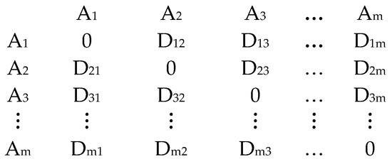
Figure 1.
The initial m x m distance matrix based on area performance scores (Pi).
In the subsequent step, the smallest value among all cells in the initial distance matrix (Figure 1) is identified. For example, if the lowest value of Dab in Figure 1 is D23 or D32 (where D23 = D32), this value is designated as the cluster distance (C.D.) for the nth round of improvement. If multiple instances of the lowest Dab values exist, any of these equal values can be selected as the cluster distance (C.D.). Once C.D. = D23 or D32 is determined, areas A2 and A3 are merged into a single group, resulting in the updated distance matrix shown in Figure 2. All values of Ea,(b,c) = E(b,c),a are computed using Equation (15) based on the maximum distance between neighboring groups. These steps are repeated iteratively to group similar areas together until the desired number of clusters is achieved.
Ea,(b,c) = E(b,c),a = max {Dab, Dac}
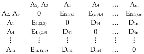
Figure 2.
The (m-1) x (m-1) distance matrix of all m areas.
2.5. Sensitivity Analysis for EntropyTOPSIS [32,33]
In the final step, the perspective weights for monthly wind speed (wp1) and agricultural areas (wp2) in Table 8 are adjusted. This adjustment, by its nature, will influence the TOPSIS performance scores (Pi) for all m areas, as it integrates both perspectives into the overall evaluation. To ensure that the clustering results for all m areas remain consistent when using the complete linkage method in Section 2.4, it is necessary to vary the values of wp1 and wp2 within a suitable range. This range can be determined by setting wp1 and wp2 based on the relationships specified in Equations (16) and (17). By adjusting these weights within the prescribed range, the integrity of the clustering outcomes from Section 2.4 is preserved, while still allowing for flexibility in how the two perspectives are weighted in the final analysis.
where 0 ≤ wp1 ≤ 1 and 0 ≤ wp2 ≤ 1
where (1) σ is the changing parameter. (2) The value of σ can be varied from 0 to . (3) The value of wp1,new is the new perspective weight of monthly wind speed. (4) The value of wp2,new is the new perspective weight of agricultural areas.
wp1 + wp2 = 1
wp1, new = σ wp1 and wp1,new + wp2,new = 1
It is important to highlight that the calculation methods described in Section 2.1, Section 2.2, Section 2.3, Section 2.4 and Section 2.5 are relatively simple and do not involve complex mathematical processes. As a result, they can be easily performed using basic computational tools. Any standard spreadsheet software that supports functions for creating, editing and analyzing datasets can be effectively employed for conducting these calculations. This accessibility ensures that the study’s analytical tasks can be carried out with minimal technical requirements, making the methodology user-friendly and adaptable for a wide range of users without the need for specialized software or advanced computational expertise. This flexibility in tool selection also facilitates efficient data manipulation, analysis and visualization, which are integral components of the research process outlined in this study.
3. Results
3.1. Initial Evaluation of Areas Based on Monthly Wind Speed Data from Dataset [26]
Most agricultural farms in Thailand use water-pumping windmills that are 9 to 15 m in height, as they operate effectively even at cut-in wind speeds as low as 3 m/s. However, research [8] suggests that for optimal performance and efficiency, the cut-in wind speed should ideally exceed 4 m/s. Based on this criterion, 28 out of 271 sub-districts on the western side of southern Thailand [26] have a minimum monthly wind speed at a height of 10 m that exceeds 4 m/s. Table 10 shows the locations of these 28 areas along with their monthly wind speeds at a height of 10 m.
Table 10.
The latitude and longitude coordinates of 28 areas (The monthly wind speed of at least 4 m/s) [26].
3.2. Determining Area Priorities for Each Perspective of Dataset Using the EntropyTOPSIS Method
Next, the dataset [26,27], which includes monthly wind speeds (Table 11) and agricultural areas (Table 12), undergoes individual analysis using Entropy–TOPSIS. The analysis begins by applying Equations (1)–(3) to the data in Table 11 and Table 12. This process assigns attribute weight values for each perspective using the Entropy Weight method, as illustrated in Table 13 and Table 14. Then, the attribute weight values for each perspective are combined with the data from Table 11 and Table 12 to produce the initial TOPSIS tables for each perspective across all 28 areas, as presented in Table 15 and Table 16. Next, Equations (4)–(10) of the TOPSIS method is applied to the data in Table 15 and Table 16. This process calculates the performance scores (Pk,i) of 28 areas for each perspective, which are then summarized in Table 17. Therefore, Table 17 should serve as the primary dataset for the subsequent analysis using the Entropy–TOPSIS method in the next step. For clearer comparison, Figure 3 displays the area prioritization results based on average wind speed, monthly wind speed and agricultural areas.
Table 11.
The monthly wind speeds at a height of 10 m of 28 areas (The monthly wind speed of at least 4 m/s) [26].
Table 12.
The agricultural areas of 28 areas [27].
Table 13.
The monthly weight values (w1,j) of monthly wind speeds at a height of 10 m.
Table 14.
The weight values (w2,j) of agricultural areas.
Table 15.
The initial TOPSIS table for monthly wind speeds at a height of 10 m of 28 areas (the monthly wind speed of at least 4 m/s) with monthly weight values.
Table 16.
The initial TOPSIS table for agricultural areas of 28 areas with area weight values.
Table 17.
The performance scores (Pk,i) for two perspectives of 28 areas.
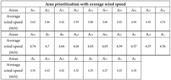

Figure 3.
Area prioritization using the average wind speed, the performance scores with monthly wind speed, and the performance scores with agricultural areas.
3.3. Establishing Area Priorities Considering a Combination of All Perspective Using the EntropyTOPSIS Method
In this process, data from Table 17 undergo an initial analysis using the entropy weight method, as described by Equations (11) and (12), to determine weighting values for two perspectives: Wp1 = 0.2212 for monthly wind speeds and Wp2 = 0.7788 for agricultural areas. Subsequently, these weights are integrated with the data from Table 17 to construct the initial TOPSIS table covering these two perspectives across all 28 areas, shown in Table 18. Following the application of Equations (4)–(9) and Equation (13) to the data in Table 18, performance scores (Pi) for all 28 areas are calculated and sorted from highest to lowest, as presented in Table 19. In Table 19, the higher performance scores indicate that an area is more suitable for installing the water-pumping windmill system compared to an area with lower scores.
Table 18.
The initial TOPSIS table for 2 perspectives of 28 areas.
Table 19.
The area performance scores (Pi) of 28 areas.
3.4. Clustering Areas Using the Complete Linkage Method
In this step, all performance scores (Pi) for all 28 areas listed in Table 18 are clustered using the complete linkage method, following Equations (14) and (15). Initially, the 28 × 28 distance matrix based on these performance scores is generated, depicted in Figure 4. After 23 iterations, the 28 areas are clustered into 6 groups with a cluster distance (C.D.) of 0.1218, illustrated in Figure 5. Subsequently, Figure 6 is created to clearly display the 6 groups: Group I, II, III, IV, V and VI. Specifically, Group I represents the most suitable areas for installing the water-pumping windmill system, characterized by very high performance scores, whereas Group VI comprises the least suitable areas with lower performance scores.
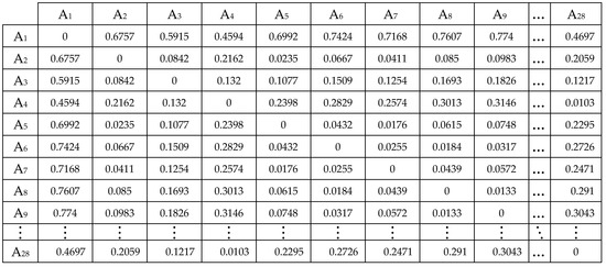
Figure 4.
The initial 28 × 28 distance matrix based on area performance scores (Pi) in Table 18.
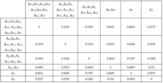
Figure 5.
The 5 × 5 distance matrix for the 23th round using the complete linkage method with C.D. = 0.1218.
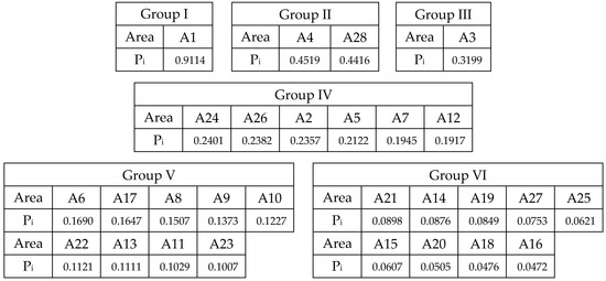
Figure 6.
The 6 area groups of 28 areas using the complete linkage method.
3.5. Sensitivity Analysis for EntropyTOPSIS [32,33]
By adjusting the weights of wp1 = 0.2212 and wp2 = 0.7788 in Table 18 according to Equations (16) and (17), the calculation results indicate that the new weights, wp1 and wp2 are related as follows: wp1,new = σ⋅wp1 and wp2,new = 1−wp1,new where σ is a variable that can range from 0 to 4.5208. It is important to note that when σ = 1, the values of wp1 and wp2 remain at their initial values of 0.2212 and 0.7788, respectively. Under these conditions, the weights wp1 and wp2 can vary within a range such that their sum always equals 1. Through sensitivity analysis, it shows that to maintain the clustering results from the complete linkage method where the 28 areas are grouped into 6 clusters with the same group members as shown in Figure 6, the value of wp1 should be adjusted within the range of 0.1749 to 0.2973. Correspondingly, wp2 should be adjusted within the range of 0.7027 to 0.8251. This adjustment ensures that the clustering results remain consistent, provided that σ is within the range of 0.7904 to 1.3438.
Since the value of σ can be adjusted within the range of 0.7904 to 1.3438 without causing any changes to the clustering results from the complete linkage method, where the 28 areas are grouped into 6 clusters with the group members as shown in Figure 6 (with σ = 1). To provide a clearer understanding of how the clustering results remain stable across this range of σ, the following sensitivity analysis is presented for two specific values of σ: σ = 0.7904 and σ = 1.3438.
- (1)
- At σ = 1 (For reference), wp1 = 0.2212 and wp2 = 0.7788, the grouping is as follows:
Group I: A1 Group II: A4, A28
Group III: A3 Group IV: A24, A26, A2, A5, A7, A12
Group V: A6, A17, A8, A9, A10, A22, A13, A11, A23
Group VI: A21, A14, A19, A27, A25, A15, A20, A18, A16
- (2)
- At σ = 0.7904, wp1 = 0.1749 and wp2 = 0.8251, the grouping is as follows:
Group I: A1 Group II: A4, A28
Group III: A3 Group IV: A2, A24, A26, A5, A7, A12
Group V: A6, A17, A8, A9, A10, A22, A13, A11, A23
Group VI: A14, A21, A27, A19, A15, A25, A18, A20, A16
- (3)
- At σ = 1.3438, wp1 = 0.2973 and wp2 = 0.7027, the grouping is as follows:
Group I: A1 Group II: A28, A4
Group III: A3 Group IV: A24, A26, A2, A5, A12, A7
Group V: A6, A17, A8, A22, A13, A9, A11, A23, A10
Group VI: A21, A19, A14, A27, A25, A20, A16, A15, A18
Table 20 presents the results of the sensitivity analysis, which show that pairwise reordering of two members within the same group occurs gradually as the value of σ adjusts (See Figure 6 for reference). Following are examples:
Table 20.
Sensitivity analysis to preserve the clustering results, where all 28 areas are clustered into 6 groups with the same group members as shown in Figure 6.
- (1)
- When σ = 0.9698, wp1 = 0.2146 and wp2 = 0.7854, the order of areas A15 and A25 in Group VI changes. Specifically, the order of area members in Group VI shifts from A21, A14, A19, A27, A25, A15, A20, A18, A16 to A21, A14, A19, A27, A15, A25, A20, A18, A16.
- (2)
- When σ = 1.0706, wp1 = 0.2369 and wp2 = 0.7631, the order of areas A7 and A12 in Group IV changes. The order in Group IV adjusts from A24, A26, A2, A5, A7, A12 to A24, A26, A2, A5, A12, A7.
Similarly, in Group VI, the order of areas A16 and A18 changes first, followed by the reordering of areas A14 and A19. The sequence of area members in Group VI is adjusted as follows:
- -
- Initially, the order changes from A21, A14, A19, A27, A25, A15, A20, A18, A16 to A21, A14, A19, A27, A25, A15, A20, A16, A18.
- -
- Subsequently, the order of areas changes again from A21, A14, A19, A27, A25, A15, A20, A16, A18 to A21, A19, A14, A27, A25, A15, A20, A16, A18.
4. Discussion
Generally, Thai farmers have relied on the average wind velocity data from Table 11 to make investment decisions for water-pumping windmill systems because this approach is straightforward and cost-effective. However, this method overlooks to consider the significant impact of seasonal variations in wind velocity. In this study, the Entropy–TOPSIS method is applied to monthly wind speed data from Table 11. The results indicate that wind speeds during the summer are notably higher than those in the rainy season, with summer wind speeds generally receiving higher weight values compared to the rainy season as shown in Table 13. Additionally, the Entropy–TOPSIS analysis of agricultural areas revealed that the quantity of agricultural area with high potential among these 28 areas is a crucial factor for area prioritization, as demonstrated by the value W2,2 = 0.6636 in Table 14. In Figure 3, prioritizing all 28 areas based on performance scores derived from monthly wind speeds, compared to using only the average wind velocity data, reveals that seasonal factors significantly affect the results. As a result, the rankings of the areas differ slightly when using monthly wind speeds versus average wind speeds. For instance, area A11 ranks first based on average wind speed data but drops to fourth when considering monthly wind speeds with seasonal variations. Conversely, area A22 ranks 23rd based on the quantity of agricultural area (Total of 3475 rai as shown in Table 12), yet it is ranked 2nd based on average wind speed and 1st based on monthly wind speed. This example suggests that areas with high wind speeds but limited agricultural potential may not be ideal for investment in water-pumping windmill systems. Therefore, it is important to analyze both monthly wind speeds and agricultural land availability together for more accurate area prioritization. To analyze both monthly wind speeds and agricultural land availability together, the Entropy–TOPSIS method is applied once more, incorporating both monthly wind speed performance scores and agricultural area performance scores. The results, presented in Table 18, reveal that agricultural areas hold significantly more weight in area prioritization compared to monthly wind speed, with a weight value of Wp2 = 0.7788. This influence affects the area prioritization, making the results in Table 19, which combine both monthly wind speed and agricultural area data, somewhat similar to the area prioritization based solely on agricultural areas shown in Figure 3.
To make the results of area prioritization in Table 19 more practical, the complete linkage clustering method is applied. Here is a summary of the process:
- (1)
- Generate dissimilarity matrix: the 28 × 28 dissimilarity matrix called the 28 × 28 initial matrix is created shown in Figure 4.
- (2)
- Apply complete linkage clustering: the clustering method is applied iteratively for 23 rounds with C.D. = 0.1218, resulting in the final clustering matrix as depicted in Figure 5.
- (3)
- Form clusters: the 28 areas were grouped into 6 clusters, as shown in Figure 6:
Group I: Area A1 (the performance score is 0.9114).
Group II: Areas A4 and A28 (the performance scores are from 0.4426 to 0.4519).
Group III: Area A3 (the performance score is 0.3199).
Group IV: Areas A2, A5, A7, A12, A24 and A26 (the performance scores are from 0.1917 to 0.2401).
Group V: Areas A6, A8, A9, A10, A11, A13, A17, A22 and A23 (the performance scores are from 0.1007 to 0.1690).
Group VI: Areas A14, A15, A16, A18, A19, A20, A21, A25 and A27 (the performance scores are from 0.0472 to 0.0898).
Considering both monthly wind speeds and agricultural areas, Group I is identified as the most suitable for investment in water-pumping windmill systems due to its ample agricultural land and adequate wind speeds. In contrast, Group VI is the least suitable, as these areas have limited agricultural land, despite having sufficient wind speeds.
To assess the robustness of the clustering results, the weights wp1 = 0.2212 and wp2 = 0.7788 are adjusted across a range of σ values from 0 to 4.5208. Within the range 0.7907 ≤ σ ≤ 1.3438, the corresponding weights 0.1749 ≤ wp1 ≤ 0.2973 and 0.7027 ≤ wp2 ≤ 0.8251 are found to maintain the clustering results from the complete linkage method, where all 28 areas are grouped into 6 clusters (Group I to Group VI) with the same group members as shown in Figure 6. However, within this range of σ, some area members may reorder within their respective groups without changing the overall cluster composition. In contrast, when σ falls below 0.7907 (With wp1 < 0.2212 and wp2 > 0.7027) or above 1.3438 (With wp1 > 0.2973 and wp2 > 0.8251), the clustering results from the complete linkage method no longer hold. In such cases, the clustering outcomes would differ from the results shown in Figure 6, indicating that the stability of the clustering structure is sensitive to values outside this range.
5. Conclusions
This study introduces a two-step Entropy–TOPSIS method in combination with the complete linkage method to prioritize and cluster areas along the west coast of Southern Thailand, based on an analysis of monthly wind speed and agricultural data. Initially, 28 out of 271 areas are selected using the criterion that the minimum monthly wind speed at a height of 10 m exceeds 4 m/s. This threshold is crucial, as water-pumping windmills, which perform most efficiently when installed at heights between 9 and 15 m, require wind speeds above 4 m/s for optimal operation. The Entropy–TOPSIS method is then applied to evaluate these 28 areas based on both monthly wind speed and agricultural land area. First, the areas are ranked individually according to their performance scores for wind speed and agricultural area. Afterward, the Entropy–TOPSIS method combines these individual performance scores into a comprehensive evaluation. The final performance scores for all 28 areas are calculated and ranked using the two-step Entropy–TOPSIS approach. In the subsequent step, the complete linkage method is used to cluster the 28 areas into 6 groups (Group I through Group VI) based on variations in wind speed quality and agricultural area quality. Areas in Group I are identified as the most suitable locations for installing water-pumping windmill systems, while those in Group VI are the least favorable. To ensure the robustness and stability of the clustering results, a sensitivity analysis is conducted. The results show that, although some area members may reorder within their respective groups, the overall composition of the six clusters remains unchanged. This demonstrates that the clustering structure is stable within the given parameters. Finally, this combined method demonstrates its practical value, primarily due to its simplicity, ease of use, and ability to consider multiple criteria (both qualitative and quantitative) simultaneously. The procedure requires no complex calculations, and only standard spreadsheet software with basic functions for data creation, editing and analysis is needed to perform the calculations. This makes the method accessible to decision makers who may not have expertise in computational analysis, while still enabling them to obtain meaningful and reliable results. Furthermore, this approach can be adapted for other decision-making processes related to sustainable energy investments in Thailand’s agriculture sector, offering a versatile tool for similar projects in the future.
Author Contributions
Conceptualization, S.K.; methodology, S.K.; software, S.K. and T.K.; validation, S.K. and T.K.; formal analysis S.K. and T.K.; writing—original draft preparation, S.K.; writing—review and editing, S.K. All authors have read and agreed to the published version of the manuscript.
Funding
This research received no external funding.
Institutional Review Board Statement
Not applicable.
Informed Consent Statement
Not applicable.
Data Availability Statement
The data presented in this study are available on request from the corresponding author. The data are not publicly available due to privacy.
Conflicts of Interest
The authors declare no conflicts of interest.
References
- Agriculture Landscape in Thailand. Available online: https://www.depa.or.th/storage/app/media/file/investment-bulletin.pdf (accessed on 1 July 2024).
- Department of Alternative Energy Development and Efficiency (DEDE). Available online: https://www.dede.go.th/ (accessed on 1 July 2024).
- Office of Agriculture Economics. Available online: https://www.oae.go.th/ (accessed on 1 July 2024).
- Agri-Map. Available online: https://www.ldd.go.th/ (accessed on 1 July 2024).
- Unchai, T.; Janyalertadum, A.; Erik Hold, A. Wind Energy Potential Assessment as Power Generation Source in Ubonratchathani Province, Thailand. Wind Eng. 2012, 36, 131–144. [Google Scholar] [CrossRef]
- Chingulpitak, S.; Wongwises, S. Critical Review of the Current Status of Wind Energy in Thailand. Renew. Sustain. Energy Rev. 2014, 31, 312–318. [Google Scholar] [CrossRef]
- Quan, P.; Leephakpreeda, T. Assessment of Wind Energy Potential for Selecting Wind Turbines: An Application to Thailand. Sustain. Energy Technol. Assess. 2015, 11, 17–26. [Google Scholar] [CrossRef]
- Prabkeao, C.; Tantrapiwat, A. Study on wind energy potential for agricultural water pumping system in the middle part of Thailand. In Proceedings of the ICEAST Conferences, Phuket, Thailand, 4–7 July 2018. [Google Scholar]
- Klongboonjit, S.; Kaitcharoenpol, T. Prioritization of Wind Energy Data with Analytical Hierarchy Process (AHP). Int. J. Intell. Eng. Syst. 2021, 14, 369–376. [Google Scholar]
- Klongboonjit, S.; Kaitcharoenpol, T. Quality Evaluation of Wind Energy Data with Complete Linkage Clustering. Int. J. Intell. Eng. Syst. 2022, 15, 456–464. [Google Scholar]
- Huang, J. Combining Entropy Weight and TOPSIS Method for Information System Selection. In Proceedings of the IEEE International Conference on Automation and Logistics, Qingdao, China, 1–3 September 2008. [Google Scholar]
- Li, X.; Wang, K.; Liu, L.; Xin, J.; Yang, H.; Gao, C. Application of the Entropy Weight and TOPSIS Method in Safety Evaluation of Coal Mines. Procedia Eng. 2011, 26, 2085–2091. [Google Scholar] [CrossRef]
- Zhengyuan, J.; XiaXia, Y. Application of Entropy Weight Method and TOPSIS Model in the Cold-chain Logistics and Distribution Center Location. Adv. Mater. Res. 2012, 569, 693–696. [Google Scholar]
- Jinxiang, F.; Lingwei, X.; Xingguan, M.; Jing, T.; Rongxin, Z.; Yuping, B.; Yulan, T.; Yunan, G. Application of Entropy Weight TOPSIS Method for Optimization of Wastewater Treatment Technology of Municipal Wastewater Treatment Plant. Nat. Environ. Pollut. Technol. 2013, 12, 285–287. [Google Scholar]
- Salehi, V.; Zarei, H.; Shirali, G.A.; Hajizadeh, K. An entropy-based TOPSIS approach for analyzing and assessing crisis management systems in petrochemical industries. J. Loss Prev. Process Ind. 2020, 67, 104241. [Google Scholar] [CrossRef]
- Qiu, Y.; Jia, S.; Liao, J.; Yang, X. Evaluation of Urban High-quality Development Level based on Entropy Weight-TOPSIS Two-step Method. J. Econ. Anal. 2022, 1, 50–65. [Google Scholar] [CrossRef]
- Fu, W.; Sun, J.; Lee, X. Research on the Openness of Digital Platforms Based on Entropy-Weighted TOPSIS: Evidence from China. Sustainability 2023, 15, 3322. [Google Scholar] [CrossRef]
- Wang, A.; An, Y.; Yu, S. Research on the Evaluation of Green Technology Renovation Measurement for Multi-Storey Houses in Severe old Regions Based on Entropy-Weight-TOPSIS. Sustainability 2023, 15, 9815. [Google Scholar] [CrossRef]
- Shekhovtsov, A.; Kizielewicz, B.; Sulabun, W. Advancing Individual Decision-Making: An Extension of the Characteristic Objects Method using Expected Solution Point. Inf. Sci. 2023, 647, 119456. [Google Scholar] [CrossRef]
- Wieckowski, J.; Watrobski, J.; Sulabun, W. Inaccuracies in Expert Judgment: Comparative Analysis of RANCOM and AHP Methods in Housing Location Selection Problem. IEEE Access 2024, 12, 142083–142100. [Google Scholar] [CrossRef]
- Wieckowski, J.; Watrobski, J.; Shkurina, A.; Sulabun, W. Adaptive Multi-Criteria Decision Making for Electric Vehicles: A Hybrid Approach Based on RANCOM and ESP-SPOTIS. Artif. Intell. Rev. 2024, 57, 270. [Google Scholar] [CrossRef]
- Wieckowski, J.; Sulabun, W. A New Sensitivity Analysis Method for Decision-Making with Multiple Parameters Modification. Inf. Sci. 2024, 678, 120902. [Google Scholar] [CrossRef]
- Kizielewicz, B.; Sulabun, W. SITW Method: A New Approach to Re-Identifying Multi-Criteria Weights in Complex Decision Analysis. Sci. Oasis 2024, 1, 215–226. [Google Scholar] [CrossRef]
- JingJing, G.; Huamin, G.; Zhiquan, L.; Feiran, H.; Junwei, Z.; Xinghua, L.; Jianfeng, M. ICRA: An Intelligent Clustering Routing Approach for UAV Ad Hoc Networks. IEEE Trans. Intell. Transp. Syst. 2023, 24, 2447–2460. [Google Scholar]
- Klongboonjit, S.; Kaitcharoenpol, T. Priority of Wind Energy in West Coast of Southern Thailand for Installing the Water Pumping Windmill System with Combining of Entropy Weight Method and TOPSIS. Energies 2023, 16, 7097. [Google Scholar] [CrossRef]
- Janjai, S. A Final Report of the Project: Development of Wind Resource Maps for Thailand; Phetkasem Printing Group: Nakhon Pathom, Thailand, 2010. [Google Scholar]
- Agricultural Area in Thailand 2022. Available online: https://webapp.ldd.go.th/lpd/node_modules/img/Download/zonmap/zonmap2/agri_zone_th.pdf (accessed on 1 July 2024).
- Rashidah, N.R.; Sabri, A.; Safiek, M. A Comparison between Single Linkage and Complete Linkage in Agglomerative Hierarchical Cluster Analysis for Identifying Tourists Segments. IIUM Eng. J. 2011, 12, 105–116. [Google Scholar] [CrossRef]
- Reinaldi, Y.; Ulinnuha, N.; Hartono, T.; Hafiyusholeh, M. Comparison of Single Linkage, Complete Linkage, and Average Linkage Methods on Community Welfare Analysis in Cities and Regencies in East Java. J. Mat. Stat. Komputas 2021, 18, 130–140. [Google Scholar] [CrossRef]
- Mamun, A.-A.; Aseltine, R.; Rajasekaran, S. Efficient Record Linkage Algorithms using Complete Linkage Clustering. PLoS ONE 2016, 11, e0154446. [Google Scholar] [CrossRef] [PubMed]
- Bulla-Cruz, L.; Lyons, L.; Darghan, E. Complete Linkage Clustering Analysis of Surrogate Measures for Road Safety Assessment in Roundabouts. Rev. Colomb. Estad.-Appl. Stat. 2021, 44, 91–121. [Google Scholar] [CrossRef]
- Triantaphyllou, E. A Sensitivity Analysis Approach for MCDM. In Multi-Criteria Decision Making Methods: A Comparative Study; Springer: Berlin/Heidelberg, Germany, 2000; pp. 131–175. [Google Scholar]
- Millek, J. The Robustness of TOPSIS Results Using Sensitivity Analysis Based on Weight Tuning. In IFMBE Proceeding: World Congress on Medical Physics and Biomedical Engineering; Springer: Berlin/Heidelberg, Germany, 2018; pp. 83–86. [Google Scholar]
Disclaimer/Publisher’s Note: The statements, opinions and data contained in all publications are solely those of the individual author(s) and contributor(s) and not of MDPI and/or the editor(s). MDPI and/or the editor(s) disclaim responsibility for any injury to people or property resulting from any ideas, methods, instructions or products referred to in the content. |
© 2024 by the authors. Licensee MDPI, Basel, Switzerland. This article is an open access article distributed under the terms and conditions of the Creative Commons Attribution (CC BY) license (https://creativecommons.org/licenses/by/4.0/).