Article

Identifying Non-Perennial River Reaches: A Hybrid Model Combining WEP-L and Random Forest

1
State Key Laboratory of Simulation and Regulation of Water Cycle in River Basin, China Institute of Water Resources & Hydropower Research, Beijing 100038, China
2
School of Hydraulic and Ecological Engineering, Nanchang Institute of Technology, Nanchang 330099, China
3
China Construction Eco-Environmental Group Co., Ltd., Beijing 100037, China
4
School of Environment and Municipal Engineering, Lanzhou Jiaotong University, Lanzhou 730070, China
*
Author to whom correspondence should be addressed.
Sustainability 2024, 16(23), 10543; https://doi.org/10.3390/su162310543
Submission received: 7 November 2024 / Revised: 28 November 2024 / Accepted: 29 November 2024 / Published: 1 December 2024
(This article belongs to the Section Sustainable Water Management)

Abstract

:
The proportion of non-perennial rivers within the global river network is increasing, and research on these rivers has significantly grown in recent years due to their important role in water resource management and ecosystems. However, existing identification methods primarily rely on river networks with monitoring data and often overlook the temporal variation in flow, limiting further research and analysis. We propose a novel identification approach that couples the WEP-L model with random forest prediction, based on a comprehensive analysis of the limitations of current methods. Specifically, this method involves simulating river flow and incorporating time-series forecasting to facilitate the identification of non-perennial rivers. This approach also divides non-perennial rivers into significantly seasonal and non-significantly seasonal rivers by incorporating seasonal analysis, providing a theoretical foundation for studying their causes and formulating conservation strategies. Using the Yellow River basin in Gansu province as a case study, the results indicate that the total length of non-perennial rivers is 13,085.67 km, accounting for 42.09% of the region’s river length. The cessation periods of significant seasonal non-perennial rivers are primarily in fall and winter, while flow periods are concentrated in summer. The findings provide valuable guidance for the ecological conservation and sustainable management of non-perennial rivers, both in the Yellow River basin and other regions. The introduction and application of this method are expected to improve the identification and management of non-perennial rivers, contributing to the long-term sustainability of water resources.

1. Introduction

Non-perennial rivers make up a high proportion of the global river network [1,2]. This proportion is continuing to rise in response to climate change and human activities [3].
In recent years, research on non-perennial rivers has gained significant momentum. Scholars have increasingly emphasized that the formation and dynamics of non-perennial rivers result from a highly complex interplay of factors, including meteorological conditions [4], river network structures [5], and anthropogenic activities [6]. The ecological significance of non-perennial rivers has gained growing recognition through detailed analyses, which have unveiled their pivotal role in ecosystem processes, species diversity, and watershed functioning. These insights challenge earlier assumptions and underscore the critical importance of these rivers [7,8]. Furthermore, an increasing number of studies have focused on examining the hydrological responses of non-perennial rivers, particularly their flow variability during drought and flood conditions. These investigations also explore strategies to mitigate the ecological impacts of such variability through the adoption of advanced watershed management practices [9,10]. Studies have also comprehensively assessed the methods of setting ecological flows in these rivers [11,12].
Despite their ecological importance, research on non-perennial rivers faces several challenges, particularly in accurately identifying and classifying these rivers due to limited monitoring data and the complex, dynamic nature of their flow regimes. Non-perennial rivers are typically recognized as rivers that seasonally cease to flow or frequently dry [13]. The primary criteria for identifying non-perennial rivers are the presence of flow cessations and the annual duration of these cessations [13,14]. However, there have been inconsistencies in the identification criteria for non-perennial rivers: thresholds for flow interruptions range from the first percentile of the average daily flow [15] to 0 m3/s, and thresholds for the duration of annual interruptions vary from one day [2] to five days [16] per year. The methods for identifying non-perennial rivers developed from these criteria can be categorized into two types: statistical analysis of historical flow data, such as directly utilizing the average duration of historical interruptions to identify non-perennial rivers [17,18], or applying Bayesian mixture models based on actual measurements from hydrological stations [19]. This type of method faces challenges in application due to the difficulty in access to low flow data and the uneven distribution of hydrological stations [20,21], thus limiting its use to the identification of main streams. Consequently, this limitation compromises the accuracy of detecting fragmented river sections, thereby hindering further research and effective watershed management efforts. The second method employs satellite imagery to identify non-perennial rivers [22]. This nascent methodology determines the presence and duration of dry riverbeds, thereby facilitating the identification of whether a river is non-perennial or not. However, due to the inherent limitations of satellite image resolution, the presence of dense vegetation, and potential inaccuracies in measuring flow rates at low water levels [16], there may be minor discrepancies. These factors may render certain river reaches difficult to identify or lead to insufficient accuracy in their characterization. Additionally, these methods seldom consider the seasonal dynamics of non-perennial rivers, despite growing recognition of their importance [13].
In order to address these challenges, this study introduces a novel approach that integrates mechanistic hydrological modeling with data-driven machine learning techniques. This methodology enables the comprehensive simulation of all rivers within a large watershed, thereby achieving full spatial coverage while effectively capturing the temporal variability in flow characteristics, even with limited monitoring data. The WEP-L model’s primary strength lies in its capacity to simulate physical hydrological processes in conjunction with the impacts of human activities, thereby providing a comprehensive representation of the hydrological cycle [23]. For instance, the WEP-L model concurrently considers natural phenomena such as precipitation, surface runoff, and groundwater recharge, as well as anthropogenic factors including agricultural irrigation, water diversion, and reservoir operations. In comparison to empirical or statistical models, the WEP-L model’s foundation in physical mechanisms provides a distinctive advantage in the capture of the complex hydrological dynamics of diverse basins. The model has demonstrated robust performance in reliably modeling stream segments, even in regions with sparse or unevenly distributed monitoring stations, and has yielded exceptional simulation results across various watersheds [24,25,26]. Moreover, the incorporation of the RF model, which utilizes the physical simulation data generated by WEP-L to predict the probability of streamflow discontinuities in river segments, enhances the predictive accuracy in data-scarce regions. This synergistic combination of physical and data-driven modeling provides a robust framework for capturing the seasonal dynamics of non-perennial rivers.
By advancing a combined modeling and machine learning approach, this study contributes to the field of hydrology by providing a more precise and scalable method for identifying non-perennial rivers, addressing both spatial and temporal data limitations. This approach lays the groundwork for sustainable water resource management by enhancing the understanding of non-perennial river dynamics and guiding ecological restoration efforts. Future research could apply this method to different climatic regions and assess its effectiveness across diverse hydrological settings, further promoting the long-term sustainability and resilience of non-perennial river systems.

2. Methods

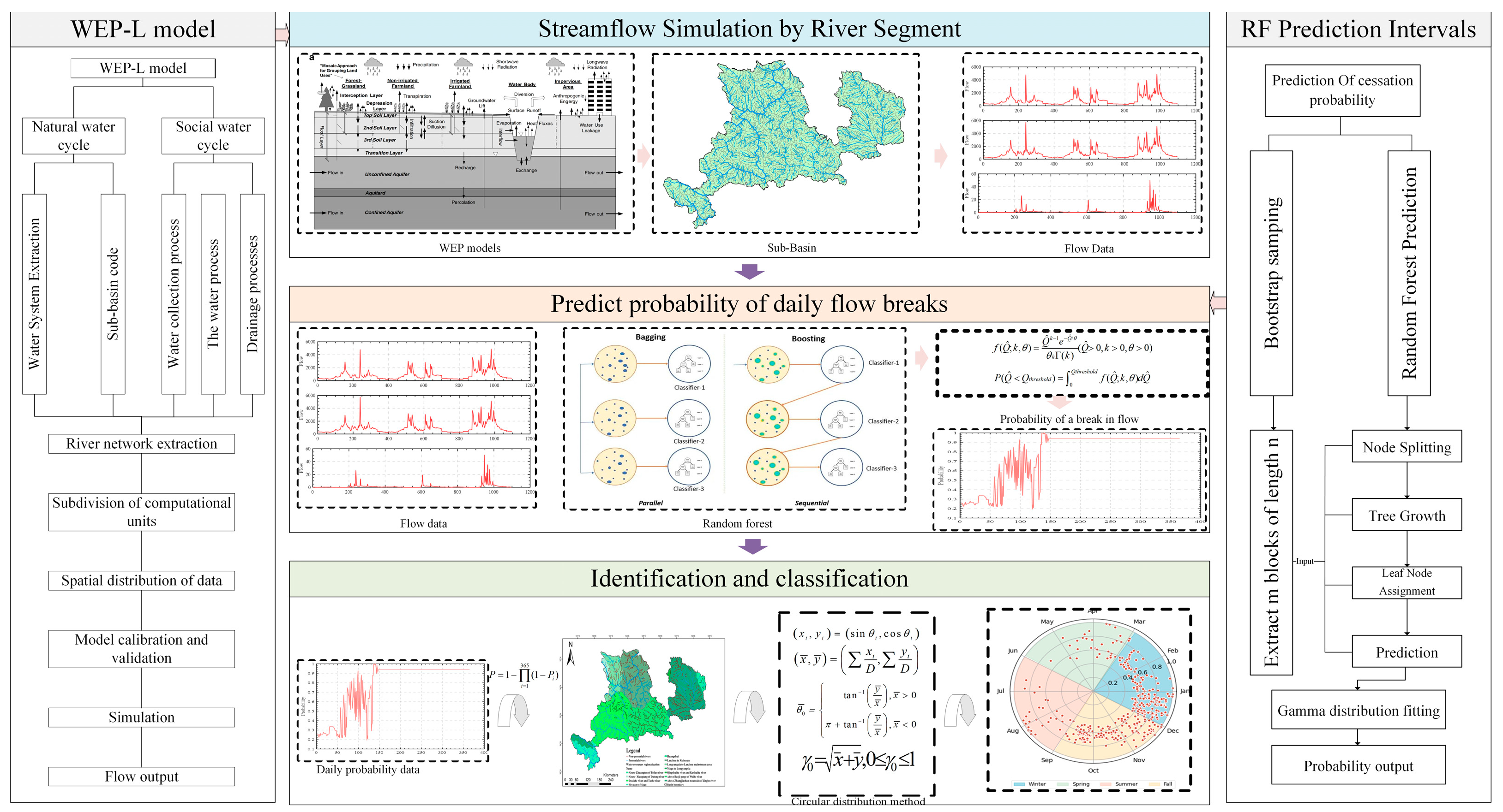
2.1. Technological Framework

The technological framework for identifying non-perennial rivers based on WEP-L and RF prediction is illustrated in Figure 1. The framework comprises the following steps: (i) WEP-L model implementation: Implementing a distributed hydrological model, WEP-L, entails the use of sub-basins nested within contour bands as the fundamental calculation units. The model is employed to simulate the natural–artificial dualistic water cycle for the basin and to generate flow data for each river segment. (ii) RF prediction: To forecast the daily probability of flow cessation, bootstrap sampling is employed on the flow data simulated by the WEP-L model for each river segment. This method entails randomly selecting blocks of N consecutive days as the training set each time to train an RF model. By repeating this process M times, M models are generated. These M models are utilized to construct daily flow prediction intervals, which are then fitted to a Gamma distribution to estimate the probability of flow cessation for each day. (iii) Identification and classification: To determine whether the river is a non-perennial river, the probability of flow cessation occurring on at least one day within a year is calculated based on daily flow cessation probabilities. Circular distribution is then used to determine if flow has significant seasonality. For non-perennial rivers without significant seasonal flow cessation, we further analyze whether their flow periods have significant seasonality. This classification divides non-perennial rivers into significantly seasonal non-perennial rivers and non-significantly seasonal non-perennial rivers. Significantly seasonal non-perennial rivers are further divided into those with significantly seasonal flow periods and those with significantly seasonal cessation periods.

2.2. WEP-L Model Implementation

The WEP-L model is a large-scale distributed hydrological model based on physical mechanisms that is utilized to couple and simulate natural water cycle processes and the impacts of human activities. The model encompasses not only natural water cycle processes, including precipitation, surface runoff, baseflow, and evaporation, but also the effects of human activities, such as reservoir regulation, canal diversion, and water allocation [27]. The basic of calculation in the WEP-L model uses the sub-basins nested within contour bands, which encompass 10 distinct types of underlying surfaces: water areas, impervious areas, bare land, forest land, grassland, sloped cropland, irrigated farmland, non-irrigated farmland, terraces, and dam areas. The general process of model establishment is as follows [28]: (i) River network extraction: To extract the simulated river network from DEM data, the slope flow accumulation method is employed. The D8 algorithm is then used to calculate raster flow direction and flow accumulation, which is subsequently used to set the threshold for extracting the river network. (ii) Computational unit division: Based on the extracted simulated river network, the watershed is divided into sub-basins and further divided into contour bands according to elevation changes within each sub-basin. (iii) Spatial distribution of data: This step can be divided into several sub-processes, mainly involving the spatial distribution of relevant data according to the subdivided calculation units (sub-basins nested within contour bands), obtaining different types of input data for each calculation unit. (iv) Model calibration and validation: This step involves calibrating highly sensitive parameters, including depression storage depth, soil saturated hydraulic conductivity, streambed material hydraulic conductivity, soil layer thickness, and stomatal resistance. The calibration process follows two standards [29]: minimizing the relative error ( R E ) and maximizing the Nash–Sutcliffe efficiency coefficient ( N S E ). The formulas for calculating these indicators are given in Equations (1) and (2). (v) Simulation: Implementing the WEP-L model for basin-specific runoff simulation aims to obtain precise and reliable results.
R E = j = 1 N Q s i m , j Q o b s , j / j = 1 N Q o b s , j × 100 %
N S E = 1 j = 1 N Q s i m , j Q o b s , j 2 / j = 1 N Q o b s , j Q o b s ¯ 2
where Q s i m , j the represents j -th simulated value, m3/s; Q o b s , j represents the j -th observed value, m3/s; N represents the number of observations; Q o b s ¯ represents the mean of the observed values flows, m3/s.

2.3. RF Prediction

The bootstrap method is a powerful resampling technique used to estimate the distribution of a statistic by sampling with a replacement from the original dataset. This approach is particularly valuable in hydrology, where datasets often exhibit temporal dependencies and variability. For each bootstrap iteration, a continuous sequence of m days is randomly drawn from a long series of length n. This selection process ensures that the temporal structure of the data is preserved, allowing the model to learn from actual sequential flows. The formula for creating a bootstrap sample can be represented as Equation (3).
S b = { Q s i m , i , Q s i m , i + 1 , , Q s i m , i + m 1 } ( i { 1 , 2 , , n m + 1 } )
This technique effectively captures the natural variability in the data by generating multiple training datasets that reflect different potential scenarios. By repeatedly drawing samples, the bootstrap method estimates the uncertainty associated with predictions, which is critical in hydrological modeling. The advantages of the bootstrap method include enhancing the model’s generalization to unseen data, effectively capturing the impacts of extreme hydrological events, and facilitating the generation of regional prediction results, thus providing valuable insights into river flow dynamics.
RF is an ensemble learning technique that constructs multiple decision trees during training and merges their predictions to enhance accuracy and stability. Each tree in the forest is built independently from the training data, promoting diversity among the trees and reducing the risk of overfitting.
The construction of each decision tree involves the following: (1) Node Splitting: Starting from the root node, the algorithm evaluates features to find the best split. The optimal threshold is determined by maximizing the reduction in impurity, often measured using metrics like Gini impurity G. For a binary classification, the Gini impurity can be expressed as Equation (4). The optimal split point is chosen to minimize impurity as Equation (5). (2) Tree Growth: Each tree is grown to its maximum depth without pruning, allowing it to learn intricate patterns from the data. While this may lead to overfitting, the ensemble nature of RF mitigates this risk by averaging predictions from multiple trees. (3) Leaf Node Assignment: Once a stopping criterion is met (e.g., reaching a maximum depth or minimum number of samples at a node), the tree assigns a prediction based on the majority class (for classification tasks) or the average value (for regression tasks) of the training data points in the leaf node. (4) Prediction: The prediction from the RF model can be mathematically expressed as Equation (6). This method’s strength lies in its ability to handle high-dimensional data and complex nonlinear relationships effectively. Each tree captures different aspects of the data, and by aggregating their outputs, RF smooths out individual errors and increases robustness against noise. This is particularly advantageous in hydrological modeling, where data can be noisy and influenced by numerous variables.
G = 1 c = 1 C p c 2
where p c is the proportion of class c at the node, and C is the total number of classes.
B e s t   S p l i t = a r g   m i n t ( G l e f t + G r i g h t )
where G l e f t denotes the impurity of the left child node and G r i g h t denotes the impurity of the right child node; a r g   m i n t indicates finding the split point c that results in the lowest combined impurity of the child nodes.
Q ^ = 1 N × j = 1 N T j ( S b )
where N is the number of trees, T j ( S b )  is the prediction from the j-th tree, and Q ^ represents the predicted flow.
To estimate the probability of daily river flow cessation, a Gamma distribution is fitted to the predicted flow intervals for each day. The Gamma distribution is renowned for its capability to model positively skewed, non-negative continuous data, making it particularly well suited for representing river flow and precipitation in hydrological datasets. Although the Pearson Type III distribution is traditionally preferred in hydrological calculations, particularly for flood frequency analysis, due to its flexibility, its computational complexity and slower fitting process present challenges. In contrast, the Gamma distribution offers greater computational efficiency and has increasingly gained attention in recent studies [30,31]. Therefore, this study employs the Gamma distribution for probabilistic estimation to leverage its efficiency and suitability for hydrological applications. Its probability density function (PDF) is given by Equation (7). The cumulative distribution function (CDF) of the Gamma distribution is then used to calculate the probability that the flow Q ^ falls below a specified threshold Q t h r e s h o l d , representing river flow cessation. In this study, the threshold for determining flow cessation was defined as a daily flow less than 0.001 m3/s, a standard that has been widely adopted in recent years due to its ability to reduce errors [32]. This probability can be expressed as Equation (8). By fitting a Gamma distribution to the predicted flow data, this approach captures the variability in daily flow rates, especially in low-flow conditions, and provides a probabilistic measure of flow cessation. The flexibility of Gamma distribution makes it well suited to handle the asymmetric nature of flow data, thus enhancing the accuracy of cessation probability estimates.
f ( Q ^ ; k , θ ) = Q ^ k 1 e Q ^ / θ θ k Γ ( k ) ( Q ^ > 0 , k > 0 , θ > 0 )
P ( Q ^ < Q t h r e s h o l d ) = 0 Q t h r e s h o l d f ( Q ^ ; k , θ ) d Q ^

2.4. Identification and Classification of Non-Perennial Rivers

2.4.1. Identification

We continued to employ the prevalent threshold for identifying non-perennial rivers, specifically using the occurrence of flow cessation on at least one day within a year as the criterion [2,3]. Using the daily probabilities of flow cessation obtained, we calculated the annual probability ( P ) that at least one day of cessation occurs, as shown in Equation (9). After the calculation, the river at P 0.5 is identified as a non-perennial river.
P = 1 i = 1 365 ( 1 P i )
where P i is the probability of flow cessation occurring on the i -th day.

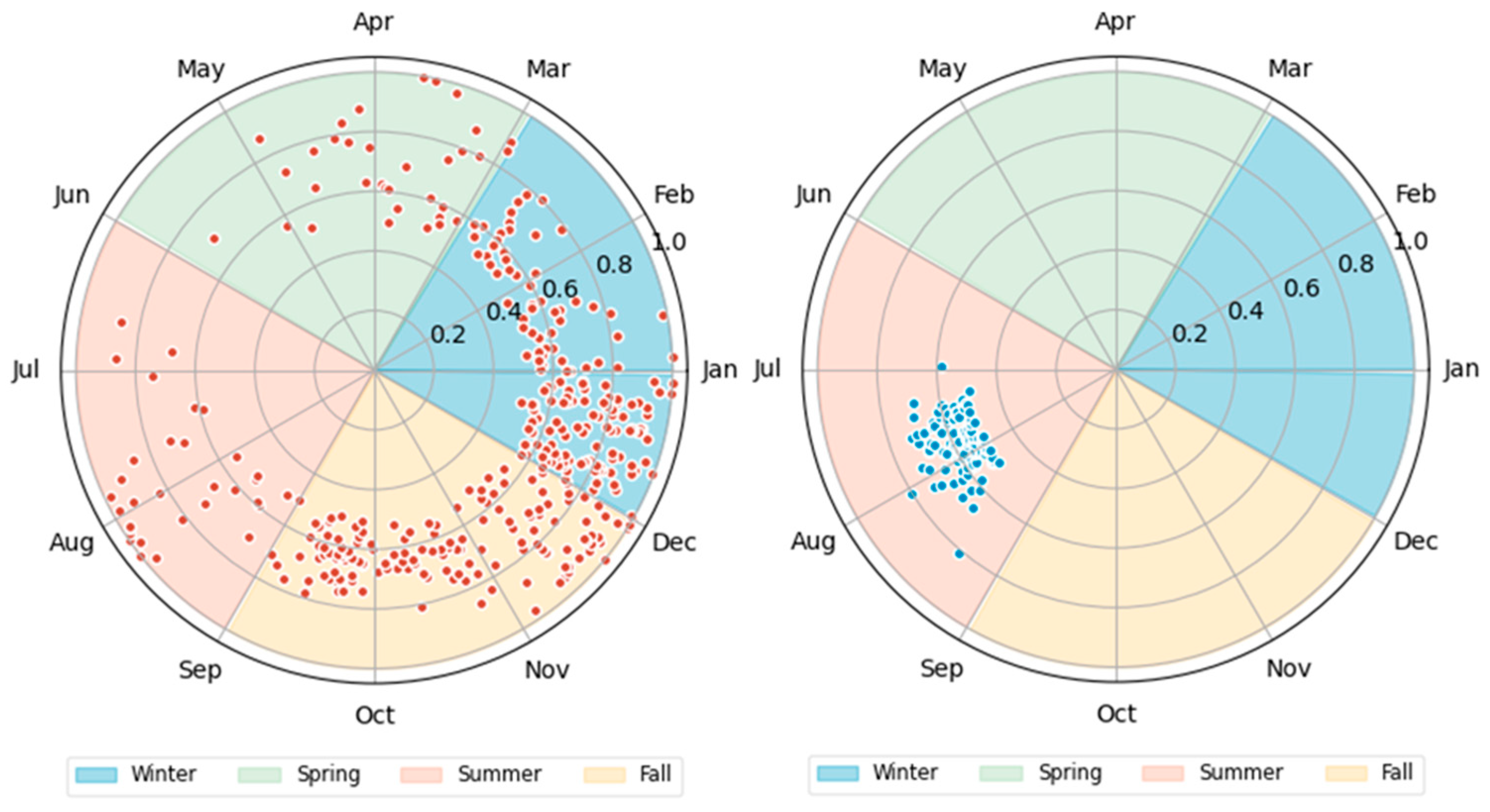
2.4.2. Classification

Based on the identification of non-perennial rivers, we further evaluate their seasonal characteristics. The circular distribution method is used to analyze the temporal patterns of river flow cessation or presence. Originally developed to determine flood seasons based on the timing of annual peak discharges [33,34], this method was subsequently adapted to describe periods of low flow below critical thresholds [35] and to characterize the concentration and focus on the cessation periods [36]. By calculating the concentration and concentrated periods of flow cessation or presence events throughout the year, we assess the significance of seasonality in non-perennial rivers. Based on this assessment, non-perennial rivers are classified into those with significantly seasonal flow periods and those with significantly seasonal cessation periods.
Days with a daily probability of flow cessation greater than the 90th percentile are identified as days with a higher probability of flow cessation. The circular distribution method is then used to identify the seasonality of these high-probability cessation days. A flow cessation concentration index ( γ 0 ) closer to 1 indicates that the high-probability cessation days are more concentrated throughout the year, suggesting stronger seasonality. In this study, a threshold of 0.5 is set to determine whether the flow cessation period exhibits significant seasonality. The specific calculation process is as follows:
High-probability cessation days are introduced into a two-dimensional coordinate system x i , y i , as shown in Equation (11). Calculate the focused period ( θ ¯ 0 ) and concentration ( γ 0 ) of high-probability cessation days within the year, as shown in Equation (13) and Equation (14).
θ i = 2 π t i T
x i , y i = sin θ i , cos θ i
x ¯ , y ¯ = x i D , y i D
θ ¯ 0 = tan 1 y ¯ x ¯ , x ¯ > 0 π + tan 1 y ¯ x ¯ , x ¯ < 0
γ 0 = x ¯ + y ¯ , 0 γ 0 1
where T is the total number of days calculated, days; t i is the date of the i -th high-probability cessation day; θ i is the time (in angles) of the i -th high-probability cessation day, 0 θ i 2 π ; D is the total number of high-probability cessation day within a year.
For non-perennial rivers with a flow cessation concentration index ( γ 0 ) less than 0.5, the study further analyzes the seasonality of their flow days. Days where the daily flow cessation probability is below the 10th percentile are identified as days with a higher probability of flow. The circular distribution method is then used to determine the seasonality of these days. The method for calculating the focused period ( θ ¯ 1 ) and concentration index ( γ 1 ) of the flow period is similar to that used for the cessation period, and will not be reiterated here. The closer the flow period concentration index ( γ 1 ) is to 1, the more concentrated the high-probability flow days are throughout the year, indicating stronger seasonality. In this study, a threshold of 0.5 is set to determine whether the flow period exhibits significant seasonality.

3. Study Area and Data

3.1. Study Area

The Yellow River basin in Gansu province is located in the upper reaches of the Yellow River and includes nine cities and prefectures including Gannan Tibetan Autonomous Prefecture, Linxia Hui Autonomous Prefecture, Lanzhou City, Baiyin City, Pingliang City, Qingyang City, Tianshui City, Dingxi City, and Wuwei City. This area serves as an important water conservation and replenishment zone for the upper reaches of the Yellow River, covering an area of approximately 142,000 square kilometers, or 34.3% of the total area of Gansu province. The Yellow River flows through this region for about 913 km, making it one of the key ecological protection areas within the Yellow River basin. It features significant ecological function zones such as the natural ecological corridor of the Yellow River, Qilian Mountains, the Loess Plateau of central Gansu, and the source of the Weihe River. The region’s terrain is complex, encompassing the Qinghai–Tibet Plateau, the Loess Plateau, Qinling–Bashan, and the Qilianshan–Hexi Corridor, resulting in a diverse ecological environment. The Yellow River basin in Gansu province is rich in water resources, with the average annual self-generated surface water resources exceeding one-fifth of the total water volume of the Yellow River basin, playing an important role in the economic and ecological development of the province.

3.2. Data Analysis

The Digital Elevation Model (DEM) of the Yellow River basin in Gansu province utilized in this study was sourced from the Global Land DEM (GTOPO30), which was created by the EROS Data Center of the US Geological Survey (USGS). GTOPO30 can be downloaded directly from the Internet at http://edcdaac.usgs.gov/gtopo30/gtopo30.asp (accessed on 28 April 2024). Meteorological data spanning from 1956 to 2018 were primarily obtained from 52 national meteorological stations. The dataset encompasses a range of variables, including precipitation, air temperature, humidity, wind speed, and sunshine hours. Furthermore, to account for the spatial heterogeneity of precipitation patterns, daily precipitation data from rainfall stations managed by the Hydrological Department were incorporated. The data pertaining to runoff were obtained from the Yellow River Conservancy Commission. Flow data for six representative cross-sections of the main and tributary rivers of the Yellow River basin in Gansu province, spanning the period from 1956 to 2016, were collated and organized.
The land use data were provided by the Institute of Geographic Sciences and Natural Resources Research, Chinese Academy of Sciences. In order to assess vegetation indices, two key indicators were employed: vegetation coverage and leaf area index (LAI). Vegetation coverage was calculated based on the Normalized Difference Vegetation Index (NDVI), which was derived from two data sources. The dataset comprised GIMMS AVHRR data (8 km resolution) from 1982 to 2006 and MOD13A2 data (1 km resolution) from 2000 to 2016. The LAI data were obtained from the GlobMap database, which provided data at an 8 km resolution from 1982 to 2005 and at a 1 km resolution from 2000 to 2015. The data on soil and water conservation were sourced from the Water Statistics Yearbook, which provides comprehensive information on soil and water conservation efforts across each county within the watershed. The statistical items analyzed included dams, terraces, planted forests, and planted grasses. Additionally, the analysis incorporated spatial and temporal data regarding changes in the characteristics of dams and terraces, as documented in the Water Statistics Yearbook for each county.
The soil characteristics were based on data from the Second National Soil Survey of China, with soil layer thickness and soil texture derived from the statistical profiles in the Soil Types of China. The hydrological parameters for the Yellow River basin in Gansu province were derived from the Water Resources Planning of the Yellow River basin. The lithology zoning and aquifer thickness data were derived from the China Hydrogeological Distribution Map. The data pertaining to irrigation areas were sourced from the Map Collections of the Yellow River basin and other materials compiled by the Yellow River Conservancy Commission. The information on water supply and consumption was primarily obtained from the survey and evaluation results of water resource development and utilization in the National Water Resources Plan.

4. Results and Discussion

4.1. Flow Simulation

The model implementation process has been thoroughly documented in the prior literature [26,27], providing a solid foundation for its application in various hydrological studies. This study focuses specifically on simulating flow variations within the Yellow River basin in Gansu province, a region characterized by complex hydrological dynamics. Using the basic computational units of the WEP-L model, the regional river network was extracted and refined, resulting in a total length of 31,087.94 km. This network was further subdivided into 1738 river segments to facilitate the accurate modeling of hydrological processes. Building on previous research, the simulation timeframe of the river segments was extended to include data through 2018, allowing for an analysis that encompasses both historical and more recent hydrological changes.
The recalibration and validation of the model was conducted using observed streamflow data from six key hydrological stations distributed throughout the study area. These stations provided a comprehensive dataset that allowed the study area to be divided into parameter zones (as shown in Figure 2). The calibration period spanned from 1956 to 1980, a period representative of historical hydrological conditions, while the validation period spanned from 1981 to 2016, ensuring that the model was tested against both historical and more recent datasets. This two-phase approach ensured a rigorous evaluation of the model’s predictive capabilities under different hydrological scenarios.
The results presented in Table 1 provide an in-depth evaluation of the model’s performance. Metrics such as relative errors (RE) and Nash–Sutcliffe efficiency coefficients (NSEs) were calculated for each station to assess the model’s accuracy and reliability. According to widely accepted hydrological model evaluation criteria [37], a model is considered to have high accuracy and efficiency when the RE is within ±10% and the NSE is greater than 0.75. In this study, the simulation results for the majority of the six hydrological stations meet these criteria. For example, the data in Table 1 show that the NSE values for Machu, Zheqiao, Xiaochuan, and Lanzhou are all above 0.75, and their RE values are close to ±10%, indicating highly accurate simulation results for these stations. For instance, the model achieved NSE values exceeding 0.75 for the majority of the stations, demonstrating strong predictive accuracy, while RE values were generally close to ±10%, indicating minimal systematic bias.

4.2. Identification of Non-Perennial Rivers

By integrating the Bootstrap algorithm with the RF model for training and prediction at the sub-basin level, a river was identified as non-perennial if the probability of having a flow rate below 0.001 m3/s for at least one day per year exceeded 0.5. As a result of this identification process, it was determined that the total length of river segments within the Yellow River basin in Gansu province that meet the specified criteria is 13,085.67 km, representing 42.09% of the total regional river network. Among the water resource regionalization in the Yellow River basin of Gansu province, the non-perennial rivers in Qingshuihe river and Kushuihe river, above Baoji gorge of Weihe river, and above Zhangjiashan mountain of the Jinghe river account for a relatively high proportion, at 96.53%, 81.50%, and 54.63%, respectively. The total length of non-perennial rivers in the area from Lanzhou to Xiaheyan is relatively high, at 2423.86 km, but the proportion is relatively low, at 38.43%. The specific distribution is shown in Figure 3.
To validate the accuracy of our results, we reference a global-scale study on the identification of non-perennial rivers [3]; this study provided maps on the global distribution of non-perennial rivers, which we used as a basis for a comparative analysis of the findings in the Yellow River basin in Gansu province. The comparison reveals that the identified non-perennial rivers in the Yellow River basin are largely consistent with those reported for corresponding regions in the global study. The consistency confirms the applicability and reliability of our method at the regional scale. Our study refines the identification of non-perennial streams by revealing detailed regional features, thereby further underscoring the advantages of applying our method at finer spatial scales.

4.3. Classification of Non-Perennial Rivers

For non-perennial rivers, a seasonal assessment was conducted using the circular distribution method. Initially, the high-probability flow cessation concentration period ( θ 0 ¯ ) and the concentration ( γ 0 ) of the higher probability of dry flow were calculated for each river section. Non-perennial rivers that exhibited a concentration ( γ 0 ) of at least 0.5 were classified as non-perennial rivers with significant seasonal flow cessation. For river sections that do not meet this standard, further calculation of the concentration period ( θ 1 ¯ ) and the concentration ( γ 1 ) of dates with higher flow probability was conducted. River sections with a concentration ( γ 1 ) of no less than 0.5 were identified as non-perennial rivers with significant seasonal flow patterns. These two types of rivers were collectively referred to as significantly seasonal non-perennial rivers. The remaining rivers were classified as non-significantly seasonal non-perennial rivers.
This process aids in further analyzing the seasonal characteristics of non-perennial rivers. The characteristic values of significantly seasonal non-perennial rivers are shown in Figure 4 The analysis results indicate that for significantly seasonal non-perennial rivers, the periods with a higher probability of flow cessation are generally concentrated in the autumn and winter seasons, whereas the periods with a higher probability of flow are concentrated in the summer.
After the above seasonal assessment and classification, a distribution map of non-perennial rivers in the Yellow River basin in Gansu province was created (Figure 5). The results show that among the non-perennial rivers, the total length of significantly seasonal non-perennial rivers is 7552.56 km, accounting for 57.72%, while the total length of non-significantly seasonal non-perennial rivers is 5533.11 km, accounting for 43.28%.

5. Conclusions

This study introduces an innovative methodology for identifying non-perennial rivers by synthesizing mechanistic simulation models with data-driven models. By coupling the WEP-L model with Random Forest (RF) prediction, this novel approach enables the precise identification of non-perennial rivers within large basins by individual segments and effectively captures temporal variations in flow dynamics. The introduction and application of this method are expected to advance the research on non-perennial rivers and promote their scientific management and protection. Furthermore, the proposed classification method for non-perennial rivers through seasonal analysis provides a theoretical framework that can guide further research and support ecological conservation efforts.
The case study of the Yellow River basin in Gansu province demonstrates that this method can effectively delineate non-perennial rivers, with a total identified length of 13,085.67 km, representing 42.09% of the river network in the region. Specifically, notable concentrations of non-perennial rivers were identified in three key water resource regions: above Baoji gorge on the Weihe River, above Zhangjiashan mountain on the Jinghe River, and from Lanzhou to Xiaheyan. In the Qingshuihe and Kushuihe river regions, 96.53% of the rivers were identified as non-perennial. The seasonal assessment revealed that flow cessation periods are predominantly concentrated during the autumn and winter, while flow periods are concentrated during the summer. These findings provide strong support for the identification and management of non-perennial rivers in the Yellow River basin and also provide useful references for the ecological protection of non-permanent rivers and the sustainable utilization and management of water resources in other regions.
Future research should focus on further optimizing the methodology and extending its verification to other river basins with different climatic conditions and hydrological characteristics. There is a need for a strengthened analysis of the factors driving non-perennial river flow, including a comprehensive investigation of the relationships between flow and environmental variables such as climate and land use. This will help address uncertainties introduced by climate change and human activities. Additionally, it is crucial to enhance our understanding of the impacts of flow transitions in non-perennial rivers on ecosystems and evaluate the effectiveness of various management strategies. By doing so, this research can provide more concrete scientific support for the conservation and ecological restoration of non-perennial rivers, ultimately contributing to their sustainable management.

Author Contributions

Writing—Original Draft, K.Y. and Z.T.; Data Curation, K.Y. and J.L.; Writing—Review and Editing, J.C., Z.Z. and Y.C.; Funding Acquisition, Y.W. All authors have read and agreed to the published version of the manuscript.

Funding

This research was funded by the Major Science and Technology Project of the Ministry of Water Resources (SKS-2022070), the Academy of Chinese Engineering S&T Strategy for development of Gansu province (GS2022ZDI02), and the project of key technology for ecological restoration of rivers and lakes (CSCEC-2022-K-36).

Institutional Review Board Statement

Not applicable.

Informed Consent Statement

Not applicable.

Data Availability Statement

The original contributions presented in the study are included in the article; further inquiries can be directed to the corresponding author.

Conflicts of Interest

Author Ying Wang was employed by the company China Construction Eco-Environmental Group Co., Ltd. The remaining authors declare that the research was conducted in the absence of any commercial or financial relationships that could be construed as a potential conflict of interest.

References

  1. Levick, L.R.; Goodrich, D.C.; Hernandez, M.; Fonseca, J.; Semmens, D.J.; Stromberg, J.C.; Tluczek, M.; Leidy, R.A.; Scianni, M.; Guertin, D.P. The Ecological and Hydrological Significance of Ephemeral and Intermittent Streams in the Arid and Semi-Arid American Southwest; US Environmental Protection Agency, Office of Research and Development: Washington, DC, USA, 2008. [Google Scholar]
  2. Snelder, T.H.; Datry, T.; Lamouroux, N.; Larned, S.T.; Sauquet, E.; Pella, H.; Catalogne, C. Regionalization of Patterns of Flow Intermittence from Gauging Station Records. Hydrol. Earth Syst. Sci. 2013, 17, 2685–2699. [Google Scholar] [CrossRef]
  3. Messager, M.L.; Lehner, B.; Cockburn, C.; Lamouroux, N.; Pella, H.; Snelder, T.; Tockner, K.; Trautmann, T.; Watt, C.; Datry, T. Global Prevalence of Non-Perennial Rivers and Streams. Nature 2021, 594, 391–397. [Google Scholar] [CrossRef] [PubMed]
  4. De Girolamo, A.M.; Barca, E.; Leone, M.; Lo Porto, A. Impact of Long-Term Climate Change on Flow Regime in a Mediterranean Basin. J. Hydrol. Reg. Stud. 2022, 41, 101061. [Google Scholar] [CrossRef]
  5. Benstead, J.P.; Leigh, D.S. An Expanded Role for River Networks. Nat. Geosci. 2012, 5, 678–679. [Google Scholar] [CrossRef]
  6. Larned, S.T.; Datry, T.; Arscott, D.B.; Tockner, K. Emerging Concepts in Temporary-river Ecology. Freshw. Biol. 2010, 55, 717–738. [Google Scholar] [CrossRef]
  7. Cid, N.; Erős, T.; Heino, J.; Singer, G.; Jähnig, S.C.; Cañedo-Argüelles, M.; Bonada, N.; Sarremejane, R.; Mykrä, H.; Sandin, L. From Meta-system Theory to the Sustainable Management of Rivers in the Anthropocene. Front. Ecol. Environ. 2022, 20, 49–57. [Google Scholar] [CrossRef]
  8. Leigh, C.; Datry, T. Drying as a Primary Hydrological Determinant of Biodiversity in River Systems: A Broad-scale Analysis. Ecography 2017, 40, 487–499. [Google Scholar] [CrossRef]
  9. Bogan, M.T.; Chester, E.T.; Datry, T.; Murphy, A.L.; Robson, B.J.; Ruhi, A.; Stubbington, R.; Whitney, J.E. Resistance, Resilience, and Community Recovery in Intermittent Rivers and Ephemeral Streams. In Intermittent Rivers and Ephemeral Streams; Elsevier: Amsterdam, The Netherlands, 2017; pp. 349–376. [Google Scholar]
  10. Pineda-Morante, D.; Fernández-Calero, J.M.; Pölsterl, S.; Cunillera-Montcusí, D.; Bonada, N.; Cañedo-Argüelles, M. Local Hydrological Conditions and Spatial Connectivity Shape Invertebrate Communities after Rewetting in Temporary Rivers. Hydrobiologia 2022, 849, 1511–1530. [Google Scholar] [CrossRef]
  11. Leone, M.; Gentile, F.; Lo Porto, A.; Ricci, G.F.; De Girolamo, A.M. Ecological Flow in Southern Europe: Status and Trends in Non-Perennial Rivers. J. Environ. Manag. 2023, 342, 118097. [Google Scholar] [CrossRef] [PubMed]
  12. Leone, M.; Gentile, F.; Lo Porto, A.; Ricci, G.F.; Schürz, C.; Strauch, M.; Volk, M.; De Girolamo, A.M. Setting an Environmental Flow Regime under Climate Change in a Data-Limited Mediterranean Basin with Temporary River. J. Hydrol. Reg. Stud. 2024, 52, 101698. [Google Scholar] [CrossRef]
  13. Busch, M.H.; Costigan, K.H.; Fritz, K.M.; Datry, T.; Krabbenhoft, C.A.; Hammond, J.C.; Zimmer, M.; Olden, J.D.; Burrows, R.M.; Dodds, W.K.; et al. What’s in a Name? Patterns, Trends, and Suggestions for Defining Non-Perennial Rivers and Streams. Water 2020, 12, 1980. [Google Scholar] [CrossRef]
  14. Smakhtin, V.U. Low Flow Hydrology: A Review. J. Hydrol. 2001, 240, 147–186. [Google Scholar] [CrossRef]
  15. Jaeger, K.L.; Sando, R.; McShane, R.R.; Dunham, J.B.; Hockman-Wert, D.P.; Kaiser, K.E.; Hafen, K.; Risley, J.C.; Blasch, K.W. Probability of Streamflow Permanence Model (PROSPER): A Spatially Continuous Model of Annual Streamflow Permanence throughout the Pacific Northwest. J. Hydrol. X 2019, 2, 100005. [Google Scholar] [CrossRef]
  16. Costigan, K.H.; Kennard, M.J.; Leigh, C.; Sauquet, E.; Datry, T.; Boulton, A.J. Flow Regimes in Intermittent Rivers and Ephemeral Streams. In Intermittent Rivers and Ephemeral Streams; Elsevier: Amsterdam, The Netherlands, 2017; pp. 51–78. [Google Scholar]
  17. Eng, K.; Wolock, D.M.; Dettinger, M.D. Sensitivity of Intermittent Streams to Climate Variations in the USA. River Res. Apps 2016, 32, 885–895. [Google Scholar] [CrossRef]
  18. Poff, N. A Hydrogeography of Unregulated Streams in the United States and an Examination of Scale-dependence in Some Hydrological Descriptors. Freshw. Biol. 1996, 36, 71–79. [Google Scholar] [CrossRef]
  19. Kennard, M.J.; Pusey, B.J.; Olden, J.D.; Mackay, S.J.; Stein, J.L.; Marsh, N. Classification of Natural Flow Regimes in Australia to Support Environmental Flow Management. Freshw. Biol. 2010, 55, 171–193. [Google Scholar] [CrossRef]
  20. Yu, S.; Bond, N.R.; Bunn, S.E.; Kennard, M.J. Development and Application of Predictive Models of Surface Water Extent to Identify Aquatic Refuges in Eastern Australian Temporary Stream Networks. Water Resour. Res. 2019, 55, 9639–9655. [Google Scholar] [CrossRef]
  21. Buttle, J.M.; Boon, S.; Peters, D.L.; Spence, C.; Van Meerveld, H.J.; Whitfield, P.H. An Overview of Temporary Stream Hydrology in Canada. Can. Water Resour. J. Rev. Can. Des Ressour. Hydr. 2012, 37, 279–310. [Google Scholar] [CrossRef]
  22. Hamada, Y.; O’Connor, B.L.; Orr, A.B.; Wuthrich, K.K. Mapping Ephemeral Stream Networks in Desert Environments Using Very-High-Spatial-Resolution Multispectral Remote Sensing. J. Arid Environ. 2016, 130, 40–48. [Google Scholar] [CrossRef]
  23. Jia, Y.; Ding, X.; Wang, H.; Zhou, Z.; Qiu, Y.; Niu, C. Attribution of Water Resources Evolution in the Highly Water-Stressed Hai River Basin of China. Water Resour. Res. 2012, 48. [Google Scholar] [CrossRef]
  24. Xu, F.; Zhao, L.; Jia, Y.; Niu, C.; Liu, X.; Liu, H. Evaluation of Water Conservation Function of Beijiang River Basin in Nanling Mountains, China, Based on WEP-L Model. Ecol. Indic. 2022, 134, 108383. [Google Scholar] [CrossRef]
  25. Wang, H.; Jiao, Y.; Hu, B.X.; Li, F.; Li, D. Study on Interaction between Surface Water and Groundwater in Typical Reach of Xiaoqing River Based on WEP-L Model. Water 2023, 15, 492. [Google Scholar] [CrossRef]
  26. Jia, Y.; Wang, H.; Zhou, Z.; Qiu, Y.; Luo, X.; Wang, J.; Yan, D.; Qin, D. Development of the WEP-L Distributed Hydrological Model and Dynamic Assessment of Water Resources in the Yellow River Basin. J. Hydrol. 2006, 331, 606–629. [Google Scholar] [CrossRef]
  27. Zhou, Z.; Liu, J.; Yan, Z.; Wang, H.; Jia, Y. Attribution Analysis of the Natural Runoff Evolution in the Yellow River Basin. Adv. Water Sci. 2022, 33, 27–37. [Google Scholar]
  28. Liu, J.J. Distributed Simulation and Evolution Law of Water Cycle in the Weihe River Basin Under Changing Environment; China Institute of Water Resources and Hydropower Research: Beijing, China, 2013. [Google Scholar]
  29. Nash, J.E.; Sutcliffe, J.V. River Flow Forecasting through Conceptual Models Part I—A Discussion of Principles. J. Hydrol. 1970, 10, 282–290. [Google Scholar] [CrossRef]
  30. Ilinca, C.; Anghel, C.G. Flood Frequency Analysis Using the Gamma Family Probability Distributions. Water 2023, 15, 1389. [Google Scholar] [CrossRef]
  31. Sabzevari, T. Runoff Prediction in Ungauged Catchments Using the Gamma Dimensionless Time-Area Method. Arab. J. Geosci. 2017, 10, 131. [Google Scholar] [CrossRef]
  32. Zimmer, M.A.; Kaiser, K.E.; Blaszczak, J.R.; Zipper, S.C.; Hammond, J.C.; Fritz, K.M.; Costigan, K.H.; Hosen, J.; Godsey, S.E.; Allen, G.H.; et al. Zero or Not? Causes and Consequences of Zero-flow Stream Gage Readings. WIREs Water 2020, 7, e1436. [Google Scholar] [CrossRef] [PubMed]
  33. Burn, D.H. Catchment Similarity for Regional Flood Frequency Analysis Using Seasonality Measures. J. Hydrol. 1997, 202, 212–230. [Google Scholar] [CrossRef]
  34. Castellarin, A.; Burn, D.H.; Brath, A. Assessing the Effectiveness of Hydrological Similarity Measures for Flood Frequency Analysis. J. Hydrol. 2001, 241, 270–285. [Google Scholar] [CrossRef]
  35. Harrigan, S.; Prudhomme, C.; Parry, S.; Smith, K.; Tanguy, M. Benchmarking Ensemble Streamflow Prediction Skill in the UK. Hydrol. Earth Syst. Sci. 2018, 22, 2023–2039. [Google Scholar] [CrossRef]
  36. Sauquet, E.; Shanafield, M.; Hammond, J.C.; Sefton, C.; Leigh, C.; Datry, T. Classification and Trends in Intermittent River Flow Regimes in Australia, Northwestern Europe and USA: A Global Perspective. J. Hydrol. 2021, 597, 126170. [Google Scholar] [CrossRef]
  37. Moriasi, D.N.; Arnold, J.G.; Van Liew, M.W.; Bingner, R.L.; Harmel, R.D.; Veith, T.L. Model Evaluation Guidelines for Systematic Quantification of Accuracy in Watershed Simulations. Trans. ASABE 2007, 50, 885–900. [Google Scholar] [CrossRef]
Figure 1. Framework for identifying and classifying non-perennial rivers based on WEP-L and RF prediction.
Sustainability 16 10543 g001
Figure 2. Map of study area.
Sustainability 16 10543 g002
Figure 3. Map of non-perennial rivers in the Yellow River basin in Gansu province.
Sustainability 16 10543 g003
Figure 4. Significant seasonal non-perennial rivers concentration distribution map. The left map shows the distribution of cessation periods for significantly seasonal non-perennial rivers with significantly seasonal cessation periods. The right map shows the distribution of flow periods for significantly seasonal non-perennial rivers with significantly seasonal flow periods.
Sustainability 16 10543 g004
Figure 5. Distribution map of two types of non-perennial rivers in the Yellow River basin in Gansu province.
Sustainability 16 10543 g005
Table 1. Efficiency coefficients for flow processes at each station.
StationRE (%)NSE
1956–19801981–20161956–20161956–19801981–20161956–2016
Machu−7.1−1.2−3.70.7880.7540.768
Zheqiao−7.610.21.40.8340.6970.796
Hongqi7.4−2.52.10.7060.6880.707
Xiaochuan−2.45.22.00.8640.6670.788
Lanzhou−2.30.9−0.40.8780.7010.809
Beidao−2.35.81.30.1440.2550.249
Disclaimer/Publisher’s Note: The statements, opinions and data contained in all publications are solely those of the individual author(s) and contributor(s) and not of MDPI and/or the editor(s). MDPI and/or the editor(s) disclaim responsibility for any injury to people or property resulting from any ideas, methods, instructions or products referred to in the content.

