Double-Layer Optimization and Benefit Analysis of Shared Energy Storage Investment Considering Life-Cycle Carbon Emission

Abstract

As a crucial path to promote the sustainable development of power systems, shared energy storage (SES) is receiving more and more attention. The SES generates carbon emissions during its manufacturing, usage, and recycling process, the neglect of which will introduce a certain extent of errors to the investment of SES, especially in the context of the large-scale integration of renewable energy and dramatic increase in demand for SES capacity. To enhance the accuracy of SES investment, we propose a double-layer optimization model to compute the optimal configuration of a shared energy storage station (SESS) considering its life-cycle carbon emission. First, the service mode, settlement method, profit mechanism, and application scenarios of SESS are introduced. Second, the life-cycle assessment approach is used to calculate the life-cycle carbon emission of SESS, and the uncertainty of supply and demand is considered. Then, a double-layer optimization model that considers the economic operation of multi-microgrid systems and the optimal allocation of SESS is established. The lower-layer model’s Karush–Kuhn–Tucher (KKT) condition is derived to convert the double-layer model into a single-layer one. Finally, a combined heat and power (CHP) three-microgrid system is used to demonstrate the validity of our proposed model, and the economy of SESS investment is analyzed from multiple perspectives. The results show that considering the life-cycle carbon emission of SESS can provide more accurate guidance for investing in and measuring the carbon emission and reduction for SESS.

1. Introduction

Electricity generation in many parts of the world is heavily reliant on fossil fuels, which emit greenhouse gases. To cut carbon emissions and alleviate air pollution in the following years, renewable energy sources have experienced significant developments in rising electricity generation and installed capacity. As indicated by data from the International Energy Agency (IEA), the total generation of renewable energy in a year is predicted to exceed 11,300 TWh by 2026 [1]. However, the increasing share of renewable energy, which is inherently uncontrollable and intermittent, presents a consumption issue for power systems.

Energy storage is a valid method to promote the consumption of renewable energy, which plays an important role in the operation and sustainable development of power systems, such as peak shaving, frequency regulation, and voltage support [2,3,4,5]. In the last few decades, energy storage technology has gained significant development, and its technical characteristics and relevant applications have been studied extensively.

1.1. Literature Review

Currently, energy storage facilities are mainly invested in and constructed by power generation companies, power grid companies, and users. However, existing energy storage facilities primarily provide service to individual entities [5,6]. This individual-based framework can meet the customized needs of an individual entity, but it has a limited utilization rate and is also economically inefficient with high investment costs, especially with the background of large-scale renewable energy integration. Therefore, the utilization rate and economy of energy storage still need to be improved.

With the growth of the sharing economy, shared energy storage (SES) has emerged [7,8]. With this new type of energy storage, users have the right to employ energy storage for specified periods by leasing energy storage without a huge investment cost. The shared energy storage station (SESS) is a typical representative of SES. The SESS investor is responsible for the investment, construction, operation, and maintenance of SESS and provides charging or discharging services for users. By utilizing the complementarity of different users’ demands during different periods, the SESS investor can minimize the required capacity of energy storage. In addition, the SESS investor can obtain a lower investment cost than energy storage invested in the distribution network with the scale benefits of SESS. For users, they can pay service fees to the SESS investor to obtain the right of using energy storage facilities, which can not only meet their own energy needs but also reduce the huge investment costs of SESS and do not necessitate complex operation and maintenance work.

The studies of SES have focused on control [9,10,11], scheduling [8,12,13,14], and planning strategy [15,16,17,18]. In terms of scheduling strategy, improving operation efficiency and reducing energy costs are the main purposes of the economic scheduling of SES for SES providers and consumers. Typically, the SES is rooted in cooperative or non-cooperative game theory, with the division of provider rights and user rights [12,13,14]. In this model, different participants utilize SES through leasing agreements. With regard to SES planning, it intends to achieve the optimal configuration of capacity and power, thus enhancing the SES utilization rate and operation performance. The issue of capacity configuration of SES is addressed within local energy communities [7,8,9,15,16,17] and intelligent buildings [18].

Carbon emission reduction has become the consensus of the entire society, and the application of energy storage is one of the crucial ways to realize this goal. However, the vast majority of studies on energy storage regard it as a zero-carbon energy source [7,8,9,10,11,12,13,14,15,16,17,18]. In fact, there is a certain amount of carbon emission during the entire life of energy storage, including manufacturing, usage in the grid, and the recycling process. The consideration of life-cycle carbon emission will enhance the accuracy of investments and decision for energy storage. It can also provide quantitative guidance for carbon emission measurement and reduction, promoting the application of energy storage. Hence, it is urgent to calculate the life-cycle carbon emission of SES, especially with the background of large-scale renewable energy integration and the dramatic increase in SES demand.

There are two main methods for calculating the life-cycle carbon emission of energy storage, which are input/output analysis (IOA) and process chain analysis (PCA) [19,20]. IOA uses the concepts of “input” and “output” to calculate the carbon emission factor, and thus, the life-cycle carbon emission is obtained. This method is easy to utilize, but it does not distinguish detailed processes, and the results are too rough. In contrast, PCA is based on detailed data from every process in the entire life, which can provide results with higher accuracy. We thus adopted PCA to compute the life-cycle carbon emission of SESS in this paper. Another method to calculate carbon emission is the carbon emission flow (CEF) method, which has been studied in [21,22,23,24]. This approach utilizes the power distribution in the grid with the carbon intensity of each machine to realize the tracking and calculation of carbon emissions. However, this method has too many assumptions and does not take into account the carbon emission during the material manufacturing and recycling process of energy storage.

The concept of life-cycle carbon emission has been introduced into the planning of building projects [25] and the optimization operation of the integrated energy system (IES) [26]. In the field of energy storage technology, the life-cycle greenhouse gas of compressed air energy storage (CAES), pumped hydro energy storage (PHES), hydrogen energy storage (HES), and multiple types of batteries has been analyzed [27,28]. These studies are pioneer efforts on the life-cycle carbon emission measurement of energy storage. However, the results obtained by these studies have not been effectively combined with energy storage investment. Note that references [23,24] introduced CEF theory into the planning of SESS, which are effective explorations in this direction. Nonetheless, both studies only considered the carbon emissions of the operation process, with too many assumptions, and a comparison of the types of energy storage is not involved. Further study is still required.

1.2. Previous Work on SESS and Research Gap

The above studies have discussed the configuration strategies of SES under different application scenarios. However, we can still notice the following limitations:

(1)

The concept of life-cycle carbon emission has not been considered in the optimization configuration of SES;

(2)

The amount of research that discusses the economy of SESS from multiple perspectives and considers different types of energy storage is relatively low.

1.3. Aims and Contributions

Our main contributions are as follows:

(1)

The concept of life-cycle carbon emission is first introduced into the investment of SESS, which considers the carbon emission of the manufacturing, operations, and recycling processes of SESS. This idea enhances the practicability and accuracy of investment strategies for energy storage;

(2)

The economy of SESS investment and the energy expenditure of electricity and heat users are considered in the double-layer optimization model, with the uncertainty of supply and demand, which contributes to the realization of a win–win situation for both sides;

(3)

The economy of SESS investment is analyzed from multiple perspectives, including net benefits, payback years, and return on investment (ROI). Moreover, the impact of considering the life-cycle carbon emission and types of energy storage on its investment is also analyzed quantitatively.

The rest of this paper is arranged as follows. Section 2 demonstrates the service mode, settlement method, profit mechanism, and application scenarios of SESS. Section 3 presents the modeling method of life-cycle carbon emission of SESS, together with the uncertainty of supply and demand. Section 4 proposes a double-layer optimization model considering the economy of SESS investment and energy expenditure of electricity and heat users in a CHP multi-microgrid system. Finally, Section 5 illustrates the effectiveness and economy of our proposed model.

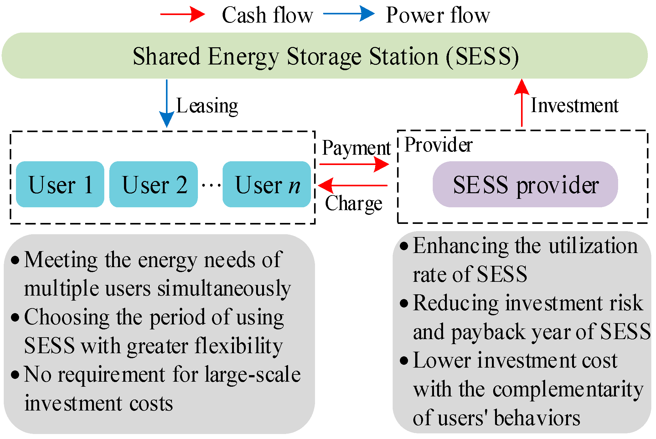
2. Shared Energy Storage Station

2.1. Service Mode of SESS

As a new type of demand-side energy storage, an SESS is an independent energy storage facility that is situated in key regions of the grid and serves all subjects of this region [29,30]. This concept originates from the shared economy, which can share the surplus power and surplus storage capacity by way of leasing, lending, or exchanging. An SESS has two attributes: “shared” and “independent”.

The attribute “shared” implies that the SESS does not just serve a single subject but provides service for multiple subjects in a power system, which can enhance the utilization hours of energy storage significantly.

The attribute “independent” means that the SESS can be invested in by a third party and participate in the trading of power market independently. Therefore, the investor and service subjects of SESS are different, which will help the social capital flow into the energy storage field and improve incentives to invest in the SESS.

Currently, financial leasing is the most common business model for SESS, the mode of which is illustrated in Figure 1. As the leaser, users have the right to use the SESS to meet their energy needs by paying the SESS provider according to leasing agreements, while the SESS provider recovers the investment cost of the SESS by charging a service fee. From the perspective of users, they do not need to invest in energy storage with high-capital costs and can avoid complex maintenance work.

From the perspective of investors, the SESS provider can utilize the complementarity feature of the power utilization of different users during different periods, which can minimize the required capacity of energy storage based on satisfying the users’ needs. In addition, the SESS provider can take advantage of the scale benefits of SESS to obtain a lower investment cost than that in the distribution network, which facilitates saving the total investment cost and reducing the payback year of the SESS.

Moreover, an SESS has significant flexibility advantages that not only can serve in the operation of large-scale power systems in cities but also have a broad range of applications in the operation of microgrids in villages and parks. This model has been employed in the operation of power systems in various countries. For example, according to the needs of public utility companies, the Edison Company proposed an energy storage leasing mode that is suitable in the field of public utilities. This model is designed to provide utility companies with a solution for line congestion and backup power support.

2.2. Settlement Method and Profit Mechanism of SESS

With the users’ historical data, electricity and heat demands, and wind power, the maximum capacity and maximum power required by users are calculated by optimizing the scheduling strategy. Based on these optimization results, the users sign a service agreement with the SESS provider. The agreement specifies the maximum charging and discharging power, rated capacity, and power output scheme required by users, and the SESS charges the users a service price. Notably, the service price refers to the fee per unit of electric power paid by users who employ the SESS to provide charging and discharging services.

Under the service agreement, the SESS provider implements the charging and discharging power scheme for each user during each period. In one period, if all the users’ demand is charging, the SESS stores the surplus power of all users. If the total demand is discharging, the SESS discharges to satisfy the needs of all users.

Users pay a service fee to purchase energy storage services from SESS, which not only meets their electricity demand but also avoids the investment, operation, and maintenance cost of energy storage completely. The service fee paid by users is based on a yearly settlement cycle, and the SESS computes the service fee by measuring the total amount of power stored in the SESS and the total amount of power released by the SESS. The sum of the two is the total cost. To contribute to the computation of the total power cost of users in a settlement cycle, the interaction power between the SESS and its users is determined in the form of power purchase and sale [29,30].

The revenue of SESS mainly includes the following: (1) the price gap between the charging and discharging process of SESS and (2) the total service fee charged by users, which is calculated according to the amount of interactive power.

2.3. Application Scenario of SESS

The SESS has a promising application in microgrids. In this paper, the combined heat and power (CHP) multi-microgrid system is used as an application scenario for the SESS, aiming to achieve the optimal configuration of the SESS and realize its value.

As shown in Figure 2, there are N CHP microgrids and one SESS in this multi-microgrid system. In a CHP microgrid, the load includes electric load and heat load, and the power supply mainly comes from the SESS, power grid, wind power, and photovoltaic (PV) grid. The heat supply mainly comes from gas turbine and gas boiler. The wind generation, PV, and power grid give priority to the requirement of electric loads, and insufficient power is purchased from the grid or supplied by the SESS.

Due to technical and political requirements, users cannot deliver power to the power grid. Therefore, we assume that users participating in the service of SESS cannot deliver power to the power grid [29]. If there is a surplus of power, the surplus power is absorbed by the SESS charging or discharging for users.

3. Life-Cycle Carbon Emission Modeling of SESS and Uncertainty of Supply and Demand

3.1. Life-Cycle Carbon Emission Modeling of SESS

For an SESS, there exists a certain amount of carbon emission during its entire life of energy storage, including the material manufacturing, usage, and recycling processes [27,28]. Hence, it is necessary to measure the life-cycle carbon emission of an SESS, especially in the context of the large-scale integration of renewable energy and dramatic increase in demand for energy storage. To specify the contributions of the SESS to the “dual-carbon” goal, we will also consider the carbon emission of an SESS from the life-cycle perspective.

In this paper, the lithium battery is first selected as the core component of SESS. During the manufacturing of the SESS, the carbon emission mainly comes from two aspects, i.e., the production of raw materials and the production and assembly of each component. The former includes the cathode plate, negative plate, and electrolyte; the latter includes the battery group, energy storage converter, etc. Therefore, the carbon emission of manufacturing SESS can be expressed as follows [28]:

$$Q_{\mathrm{Ess},\mathrm{manu}}=E_{\mathrm{Ess},\mathrm{rate}}({\mu }_{\mathrm{Ess},\mathrm{pro}}+{\mu }_{\mathrm{Ess},\mathrm{raw}})$$

(1)

where Q_Ess,manu is the carbon emission of the manufacturing process of the SESS; μ_Ess,pro is the carbon emission coefficient of the component production and assembly; μ_Ess,raw is the carbon emission coefficient of the raw materials production; E_Ess,rate is the rated capacity of the SESS.

In the usage process of the SESS, the total carbon emission is positively proportional to the rated storage capacity of the SESS, which can be represented as follows [28]:

$$Q_{\mathrm{Ess},\mathrm{use}}=E_{\mathrm{Ess},\mathrm{rate}}{\mu }_{\mathrm{Ess},\mathrm{use}}$$

(2)

where Q_Ess,use is the carbon emission of the usage process of the SESS; μ_Ess,use is the carbon emission coefficient of the usage process of the SESS.

When the SESS is retired, its components can be recycled, and its carbon emission can be reduced if recyclable components are effectively used. The carbon emission of the SESS in the recycling process can be denoted as follows [28]:

$$Q_{\mathrm{Ess},\mathrm{re}}={\mu }_{\mathrm{re},\mathrm{y}}{\eta }_{\mathrm{re}}{E}_{\mathrm{Ess},\mathrm{rate}}+{\mu }_{\mathrm{re},\mathrm{n}}(1-{\eta }_{\mathrm{re}})E_{\mathrm{Ess},\mathrm{rate}}$$

(3)

where Q_Ess,re is the carbon emission of the recycling process of the SESS; μ_re,y is the carbon emission coefficient when the components of the SESS can be effectively recycled; μ_re,n is the carbon emission coefficient when the components of the SESS cannot be effectively recycled; η_re is the effective recovery efficiency of the components of the SESS.

In summary, assume that the life cycle of SESS is m years, and the number of operation days of the SESS in one year is T_d, then the average daily carbon emission cost C_Ess,carb,i of SESS on the ith typical day is as follows:

$$C_{\mathrm{Ess},\mathrm{carb},i}={\displaystyle \frac{c_{\mathrm{carb}}(Q_{\mathrm{Ess},\mathrm{manu}}+Q_{\mathrm{Ess},\mathrm{use}}+Q_{\mathrm{Ess},\mathrm{re}})}{m{T}_{\mathrm{d}}}}={\displaystyle \frac{c_{\mathrm{carb}}\mu E_{\mathrm{Ess},\mathrm{rate}}}{m{T}_{\mathrm{d}}}}$$

(4)

where c_carb is the price of carbon emission, and $\mu ={\mu }_{\mathrm{Ess},\mathrm{pro}}+{\mu }_{\mathrm{Ess},\mathrm{raw}}+{\mu }_{\mathrm{Ess},\mathrm{use}}+{\mu }_{\mathrm{re},\mathrm{y}}{\eta }_{\mathrm{re}}+{\mu }_{\mathrm{re},\mathrm{n}}(1-{\eta }_{\mathrm{re}})$.

3.2. Uncertainty of Supply and Demand

Since wind and PV power have obvious intermittency and fluctuations, and the user’s electricity consumption behavior also has strong randomness, the predicted power of supply and demand often has a certain degree of error. For this end, the normal distribution is used to formulate the prediction error [31,32]:

$${\Delta }_t\sim N(0,k_1{P}_{t,\mathrm{pre}}+k_2{P}_{t,\max })$$

(5)

where Δ_t is the error of the predicted power of supply and demand at period t; P_t,pre is the predicted power of supply and demand at period t; P_t,max is the maximum predicted power of supply and demand at period t; k₁ and k₂ are error coefficients.

The actual power of supply and demand is the sum of the power prediction and prediction error, which can be expressed as follows [31,32]:

$$P_{t,\mathrm{real}}=P_{t,\mathrm{pre}}+{\Delta }_t$$

(6)

where P_t,real is the actual power of supply and demand at period t.

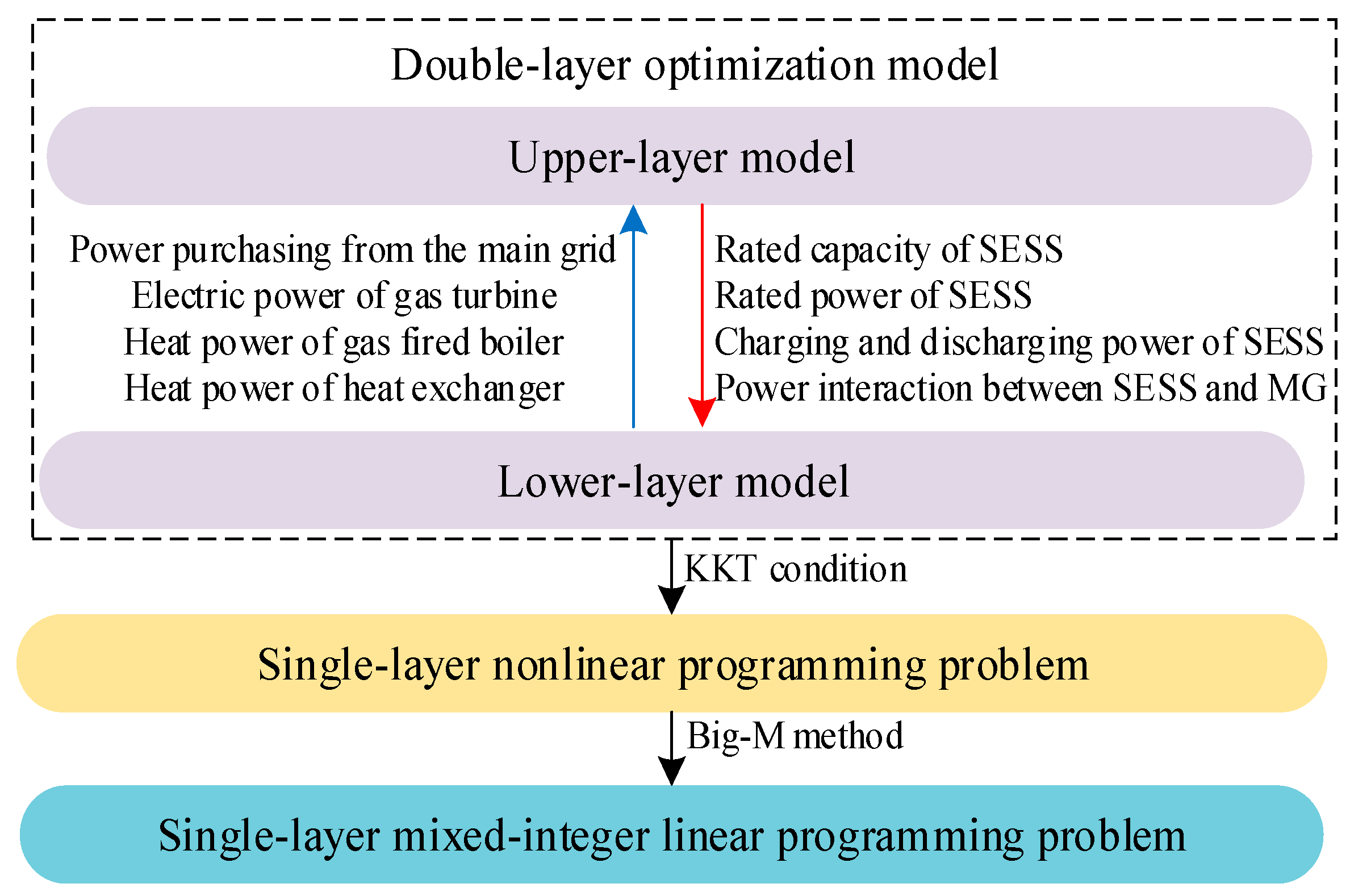
4. Double-Layer Optimization Model Considering Life-Cycle Carbon Emission of SESS

The upper-layer and lower-layer models are from the perspective of investors and users, respectively. To be specific, the upper-layer model takes priority in decision making and passes the values of decision variables to the lower-layer model. The lower-layer model determines the feasible domain according to the results of upper-layer model and calculates the optimal results. Then, the optimal values of the lower-layer model are transferred to the upper-layer model. Through several iterations, we can obtain the optimal solutions of the upper-layer and lower-layer models.

The advantage of the double-layer optimization model is that it can consider the benefits of the upper-layer and lower-layer subjects simultaneously, which contributes to a win–win situation for both sides.

4.1. Upper Layer: Optimal Configuration of SESS

The upper-layer model aims to minimize the annual operation cost of the SESS in the day-ahead electricity market, whose decision variables consist of the rated capacity, rated power, charging and discharging power of SESS, and power interaction between SESS and each microgrid. The objective function of upper-layer model C_T can be denoted as follows:

$$\min C_{\mathrm{T}}={\displaystyle \sum _{i=1}^I{T}_i[C_{\mathrm{Inv},i}+C_{\mathrm{Main},i}+C_{\mathrm{Grid},\mathrm{Ess},i}+C_{\mathrm{Ess},\mathrm{Carb},i}-C_{\mathrm{Serve},i}]}$$

(7)

where I is the number of typical day in a year; T_i is the number of days corresponding to the ith typical day; C_Inv,i, C_Main,i, C_Grid,Ess,i, and C_Serve,i are the daily investment cost, daily operation and maintenance cost, daily power interaction cost, and daily service revenue of the SESS on typical day i, respectively.

(1)

Daily investment cost of SESS

$$C_{\mathrm{Inv},i}={\displaystyle \frac{c_{\mathrm{P}}{P}_{\mathrm{Ess},\mathrm{rate}}+c_{\mathrm{E}}{E}_{\mathrm{Ess},\mathrm{rate}}}{m{T}_{\mathrm{d}}}}$$

(8)

where c_P and c_E are the unit power price and unit capacity price of the SESS, respectively; P_Ess,rate is the rated power of the SESS.

(2)

Daily operation and maintenance cost of the SESS

$$C_{\mathrm{Main},i}=c_{\mathrm{Main}}{P}_{\mathrm{Ess},\mathrm{rate}}$$

(9)

where c_Main is the daily maintenance price of the SESS.

(3)

Daily interactive power cost of the SESS [30]

$$C_{\mathrm{Grid},\mathrm{Ess},i}={\displaystyle \sum _{n=1}^N{\displaystyle \sum _{t=1}^T[c_{\mathrm{Grid}}(t)P_{\mathrm{Grid},i,n}(t)}}]$$

(10)

where N is the number of microgrids; T is the total periods in a scheduling cycle; c_Grid(t) is the power interaction price between the SESS and microgrid at period t; P_Grid,i,n(t) is the power interaction between the SESS and microgrid n at period t on typical day i; P_Grid,i,n(t) > 0 shows that the SESS purchases power from the microgrid n at period t on typical day i, P_Grid,i,n(t) < 0 shows that the SESS sells power to the microgrid n at period t on typical day i.

(4)

Daily service revenue of the SESS [30]

$$C_{\mathrm{Serve},i}={\displaystyle \sum _{n=1}^N{\displaystyle \sum _{t=1}^T[c_{\mathrm{Serve}}(t)P_{\mathrm{Grid},i,n}(t)]}}$$

(11)

where c_Serve(t) is the service price charged by the microgrid at period t.

The upper-layer model has the following constraints:

(1)

Capacity/power ratio constraint [33]

$$E_{\mathrm{Ess},\mathrm{rate}}=\alpha P_{\mathrm{Ess},\mathrm{rate}}$$

(12)

where α is the energy ratio of the SESS.

(2)

State constraints [30]

$$\left\{\begin{array}{l}{E}_{\mathrm{Ess}}\left(t)=E_{\mathrm{Ess}}\right(t-1)+[{\eta }_{\mathrm{C}}{P}_{\mathrm{Ess},\mathrm{C}}\left(t\right)-P_{\mathrm{Ess},\mathrm{D}}\left(t\right)/{\eta }_{\mathrm{D}})]\\ E_{\mathrm{Ess}}\left(0\right)=0.2E_{\mathrm{Ess},\mathrm{rate}}\\ 0.1E_{\mathrm{Ess},\mathrm{rate}}\le E_{\mathrm{Ess}}\left(t\right)\le 0.9E_{\mathrm{Ess},\mathrm{rate}}\end{array}\right.$$

(13)

where E_Ess(t) is the electricity storage of the SESS at period t; E_Ess(0) is the initial energy storage of the SESS; η_C and η_D are the efficiency of the SESS charging and discharging, respectively.

(3)

Power output constraints [30]

$$\left\{\begin{array}{l}0\le P_{\mathrm{Ess},\mathrm{C}}\left(t\right)\le U_{\mathrm{C}}\left(t\right)P_{\mathrm{Ess},\mathrm{rate}}\\ 0\le P_{\mathrm{Ess},\mathrm{D}}\left(t\right)\le U_{\mathrm{D}}\left(t\right)P_{\mathrm{Ess},\mathrm{rate}}\\ U_{\mathrm{C}}\left(t\right)+U_{\mathrm{D}}\left(t\right)\le 1\end{array}\right.$$

(14)

where P_Ess,C(t) and P_Ess,D(t) are the power of the SESS charging and discharging at period t, respectively; U_C(t) and U_D(t) are the states of the SESS charging and discharging at period t, respectively.

4.2. Lower Layer: Optimization Scheduling of CHP Multi-Microgrid System

The lower-layer model is intended to minimize the annual operation cost of the CHP multi-microgrid system, whose decision variables include the power purchasing from the main grid, electric power of the gas turbine, heat power of the gas-fired boiler, and heat power of the heat exchanger. The objective function of the lower-layer model C_L is represented as follows:

$$\min C_{\mathrm{L}}={\displaystyle \sum _{i=1}^I{T}_i(C_{\mathrm{MG},\mathrm{buy},i}+C_{\mathrm{Fuel},i}-C_{\mathrm{Grid},\mathrm{Ess},i}+C_{\mathrm{Serve},i})}$$

(15)

where C_MG,buy,i is the power-purchasing cost of all microgrids from the main grid on typical day i; C_Fuel,i is the gas cost of the gas turbine and gas-fired boiler of all microgrids on typical day i.

(1)

Daily power cost of microgrid purchasing from the main grid [29]

$$C_{\mathrm{MG},\mathrm{buy},i}={\displaystyle \sum _{n=1}^N{\displaystyle \sum _{t=1}^T[c_{\mathrm{MG},\mathrm{buy}}(t)P_{\mathrm{MG},\mathrm{buy},i,n}(t)}}]$$

(16)

where c_MG,buy(t) is the power-purchasing price of the microgrid from the main grid at period t; P_MG,buy,i,n(t) is the purchasing power of microgrid n from the main grid at period t on typical day i.

(2)

Daily gas-purchasing cost of the microgrid [29]

$$C_{\mathrm{fuel},i}=C_{\mathrm{GT},i}+C_{\mathrm{EB},i}$$

(17)

$$C_{\mathrm{GT},i}=c_{\mathrm{Gas}}{\displaystyle \sum _{n=1}^N{\displaystyle \sum _{t=1}^T{P}_{\mathrm{GT},i,n}(t)/{\eta }_{\mathrm{GT}}{L}_{\mathrm{Gas}}}}$$

(18)

$$C_{\mathrm{GB},i}=c_{\mathrm{Gas}}{\displaystyle \sum _{n=1}^N{\displaystyle \sum _{t=1}^T{Q}_{\mathrm{GB},i,n}(t)/{\eta }_{\mathrm{GB}}{L}_{\mathrm{Gas}}}}$$

(19)

where c_Gas is the gas price; L_gas is the calorific gas value; P_GT,i,n(t) is the electric power of the gas turbine in microgrid n at period t on typical day i; Q_GB,i,n(t)is the heat power of the gas-fired boiler in microgrid n at period t on typical day i; η_GT and η_GB are the efficiency of the gas turbine and gas-fired boiler, respectively.

The lower-layer model needs to meet the following constraints:

(1)

Electric power balance constraint

$$P_{\mathrm{GT},i,n}(t)+P_{i,n,\mathrm{real}}^{\mathrm{WT}}(t)+P_{i,n,\mathrm{real}}^{\mathrm{PV}}(t)+P_{\mathrm{MG},\mathrm{buy},i,n}(t)=P_{i,n,\mathrm{real}}^{\mathrm{Load}}(t)+P_{\mathrm{Grid},i,n}(t)$$

(20)

where $P_{i,n,\mathrm{real}}^{\mathrm{WT}}(t)$ is the actual wind power of microgrid n at period t on typical day i; $P_{i,n,\mathrm{real}}^{\mathrm{PV}}(t)$ is the actual PV power of microgrid n at period t on typical day i; $P_{i,n,\mathrm{real}}^{\mathrm{Load}}(t)$ is the actual electric load of microgrid n at period t on typical day i.

(2)

Heat power balance constraint

$$Q_{\mathrm{GB},i,n}(t)+Q_{\mathrm{HX},i,n}(t)=Q_{i,n,\mathrm{real}}^{\mathrm{Heat}}(t)$$

(21)

where Q_HX,i,n(t) is the heat power of the heat exchanger of microgrid n at period t on typical day i; $Q_{i,n,\mathrm{real}}^{\mathrm{Heat}}(t)$ is the actual heat load of microgrid n at period t on typical day i.

(3)

Heat power balance constraint of the waste heat boiler [29]

$${\displaystyle \frac{Q_{\mathrm{HX},i,n}(t)}{{\eta }_{\mathrm{HX}}}}-{\beta }_{\mathrm{GT}}{\eta }_{\mathrm{HRSB}}{P}_{\mathrm{GT},i,n}(t)=0$$

(22)

where η_HX is the efficiency of the heat exchanger; β_GT is the ratio of heat and electricity of the waste heat boiler; η_HRSB is the efficiency of the waste heat boiler.

(4)

Charging and discharging power balance constraint of SESS [30]

$${\displaystyle \sum _{n=1}^N{P}_{\mathrm{Grid},i,n}(t)}=P_{\mathrm{Ess},\mathrm{D}}>(t)-P_{\mathrm{Ess},\mathrm{C}}>(t>)$$

(23)

(5)

Output constraints of equipment in the CHP multi-microgrid system [29]

$$\left\{\begin{array}{l}{P}_{\mathrm{GT},\min }\le P_{\mathrm{GT},i,n}(t)\le P_{\mathrm{GT},\max }\\ Q_{\mathrm{GB},\min }\le Q_{\mathrm{GB},i,n}(t)\le Q_{\mathrm{GB},\max }\\ Q_{\mathrm{HX},\min }\le Q_{\mathrm{HX},i,n}(t)\le Q_{\mathrm{HX},\min }\end{array}\right.$$

(24)

where P_GT,max and P_GT,min are the maximum and minimum output of the gas turbine, respectively, Q_GB,max and Q_GB,min are the maximum and minimum output of the gas-fired boiler, respectively; Q_HX,max and Q_HX,min are the maximum and minimum generation of the heat exchanger, respectively.

(6)

Purchasing power of the microgrid from the main grid [29]

$$0\le P_{\mathrm{MG},\mathrm{buy},i,n}(t)\le P_{\mathrm{MG},\mathrm{buy},\max }$$

(25)

where P_MG,buy,max is the maximum purchasing power of the microgrid from the main grid.

(7)

Interactive power between the CHP multi-microgrid system and the SESS [29]

$$-P_{\mathrm{Grid},\max }\le P_{\mathrm{Grid},i,n}(t)\le P_{\mathrm{Grid},\max }$$

(26)

where P_Grid,max is the maximum power interaction of the SESS and microgrid.

4.3. Model Solution Strategy

Methods based on Karush–Kuhn–Tucker (KKT) condition [18,34,35] and meta-heuristic algorithms [36] are suitable to solve double-layer optimization problems. However, meta-heuristic algorithms are prone to falling into local optimality, and the computational efficiency cannot be guaranteed. Hence, we use methods based on the KKT condition to solve double-layer optimization problems.

Note that there are no integer variables in the lower-layer model. Based on KKT condition of the lower-layer model, the lower-layer model can be transformed into the constraints of the upper-layer model, which was derived in references [18,34,35] and is not presented further here.

To deal with nonlinear terms in the upper-layer model, we use the Big-M method in [30,35,37] to convert the nonlinear terms into linear ones. As such, the double-layer optimization model was converted into a mixed-integer linear optimization problem that can be solved via CPLEX solver and YALMIP toolbox in Matlab 2022a.

The detailed solution steps of the proposed double-layer optimization model are shown in Figure 3.

5. Case Study

5.1. Case Description

In this section, we select a CHP multi-microgrid system consisting of three CHP microgrids (N = 3), including MG₁, MG₂, and MG₃, as depicted in Figure 2. The power interaction price between the SESS and microgrid and the power-purchasing price of each microgrid from the main grid are provided in Figure 4.

In a year, there are four typical days, namely spring, summer, autumn, and winter days; the number of the ith typical day is T_i = 91; T_d = 364. The time of spring, summer, autumn, and winter is from March to May, June to August, September to November, and December to February, respectively.

There are 24 periods in a day; i.e., T = 24. The predicted electricity and heat loads of different typical days are provided in Figure 5. The predicted wind power and PV of different typical days are provided in Figure 6, and the error coefficients k₁ = k₂ = 0.02. Note that there is no wind generation in the MG₂. The transformed mixed-integer linear optimization problem is solved via CPLEX solver and YALMIP toolbox in Matlab 2022a.

Other parameters are as follows [29]: L_gas = 9.7 kWh/m³, c_Gas = 2.2 CNY/m³, c_Serve = 0.05 CNY/kWh, η_GT = 0.3, η_GB = 0.9, η_HX = 0.9, η_HRSB = 0.8, β_GT = 1.47, P_GT,max = 2000 kW, P_GT,min = 0, Q_GB,max = 2000 kW, Q_GB,min = 0, Q_HX,max = 2000 kW, Q_HX,min = 0, P_MG,buy,max = 2000 kW, and P_Grid,max = 2000 kW.

Compared with a lead-acid battery, a lithium battery has a higher energy density and a longer cycle life. Moreover, the lithium battery has higher charging efficiency without too-high investment costs compared to a vanadium-redox battery. Hence, the lithium battery is first selected as the core component of SESS, whose parameters are provided in

Table 1. Parameters of different types of energy storage [28,38,39].

Battery Type	cP (CNY/kW)	cE (CNY/kWh)	cMain (CNY/kW)	ηC/ηD	m/Year	Μ (kgCO2/kWh)
Lithium battery	2234	1173	97	0.9/0.8	15	136.76
Lead-acid battery	650	1200	25	0.8/0.9	10	85.53
Vanadium-redox battery	3720	1085	186	0.7/0.8	20	148.45

. The economic analysis of selecting a lead-acid battery or a vanadium-redox battery as core components of SESS is shown in Section 5.3.

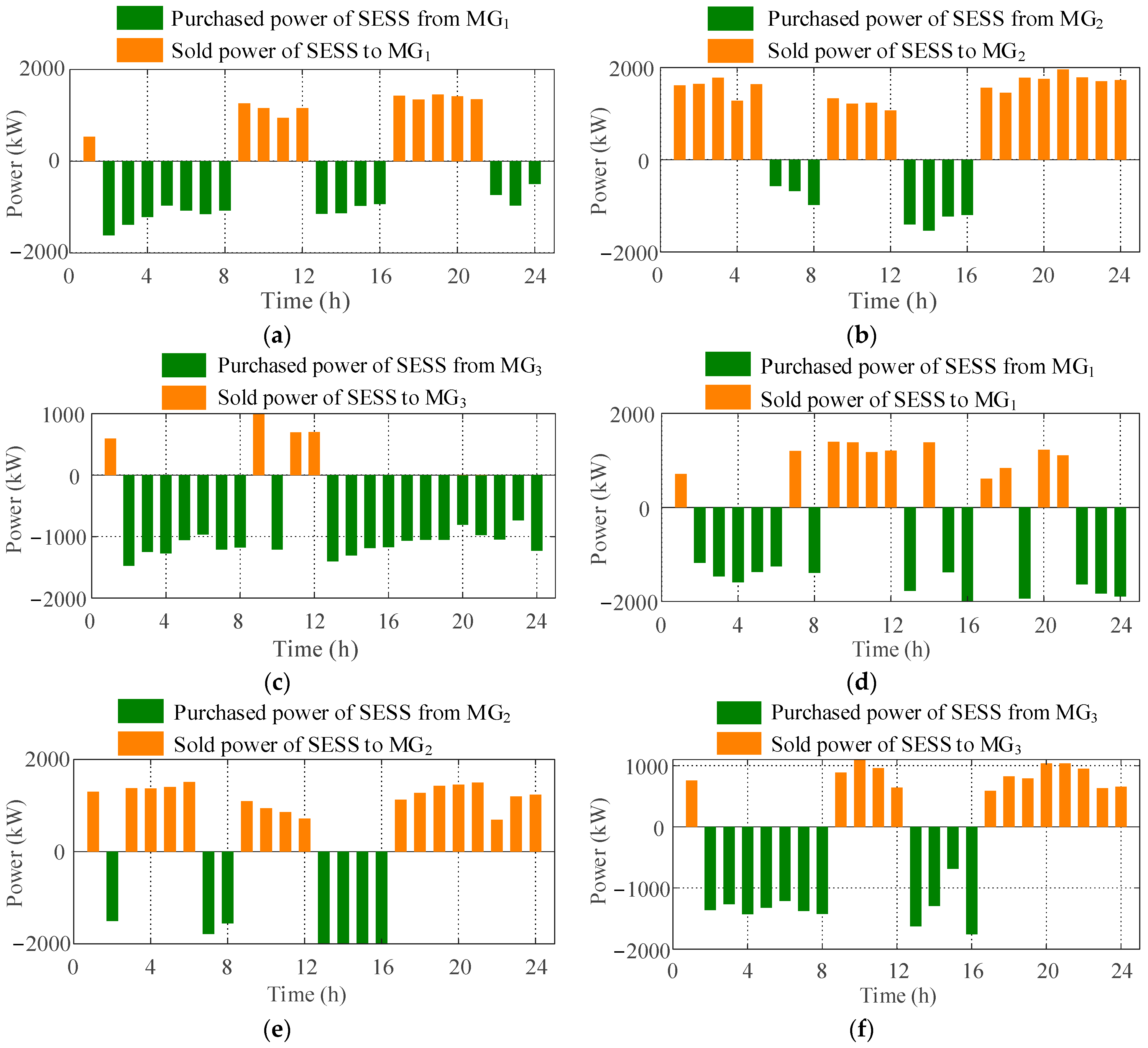
5.2. Results and Analysis

In this section, the results of the optimal configuration of SESS are first analyzed, together with the optimal charging and discharging power, and the energy storage of the SESS on typical days. Then, the interactive power between SESS and each microgrid is provided and analyzed. At last, we analyze the relationship between the annual revenue, service charge revenue, and the service price of SESS since the service charge is an important way of the revenue of SESS.

When the CHP multi-microgrid system participates in the service of the SESS, the optimal charging and discharging output and energy storage of the SESS on typical days in summer and winter are given in Figure 7a–d, respectively. Positive power means that the SESS is charging, whereas negative power means that the SESS is discharging.

By solving the transformed single-layer mixed-integer linear programming problem, the rated power and rated capacity of SESS are 7420.04 kW and 19,780.35 kWh, respectively. Figure 7a,b show that on a typical summer day, the SESS reaches the maximum charging power during 12:00–13:00 to absorb the surplus power of each microgrid. The discharging power is at the highest level in the course of 8:00–9:00, which is intended to meet the users’ demand during peak-load hours. The optimal charging and discharging power are closely associated with the characteristics of the electricity users, wind, and PV output. In addition, the SESS is always charging during 1:00–8:00 and 12:00–16:00, and its maximum electricity storage is 14,925.53 kWh, reaching the maximum power capacity of 0.9E_Ess,rate. On a typical winter day, the maximum charging, discharging power, and energy storage are 5767.76 kW, 3901.65 kW, and 16,683.01 kWh, respectively.

Figure 7c,d show that on a typical winter day, the SESS is still charging during 1:00–8:00 and 12:00–16:00 since MG₁, MG₂, and MG₃ have large amounts of surplus power during these periods. During peak-load hours, such as 8:00–12:00 and 16:00–21:00, the SESS is in the discharging state to supply the users’ demand. Moreover, the energy storage of the SESS always remains between 0.1E_Ess,rate and 0.9E_Ess,rate, satisfying its storage state constraints.

The power interaction between the SESS and each microgrid on typical days in summer and winter is illustrated in Figure 8a–f, respectively.

As can be seen in Figure 8a–c, on a typical summer day, the wind and PV output of microgrid MG₃ is larger than the local loads’ level. To avoid wind and PV abandonment, all surplus power is absorbed by the SESS. In contrast, since microgrid MG₂ has no wind power, its electricity load demand cannot be satisfied only with local PV generation. Hence, MG₂ needs to buy large amounts of electricity from the SESS to meet the users’ demand. The maximum purchased power is 1909.00 kW, and the average purchased power in each period is 1121.45 kW. From Figure 8d–f, on a typical winter day, we notice that the maximum purchased power of MG₂ from the SESS and its average value are 1549.92 kW and 897.16 kW, respectively, which is still at a high level.

The service charge of the SESS is an important source of its revenue. To this end, the relationship between the annual revenue, service charge revenue, and the service price of SESS is analyzed, whose results are shown in Figure 9.

As can be seen in Figure 9, the annual service charge revenue of SESS is positively related with the service price. When the service price is 0.05 CNY/kWh, the annual service charge revenue of SESS is 158.61 ten thousand CNY. When the service charge price is 0.15 CNY/kWh, the annual service charge revenue of SESS is 483.93 ten thousand CNY. In addition, with the growth of service price, the annual revenue of SESS also increases, and the growth is greater than that of annual service revenue. This is mainly because the growth of the service charge price will also bring about an additional increase in the rated capacity and rated power of the SESS.

5.3. Economic Evaluation of SESS Investment and Impact of Life-Cycle Carbon Emission on SESS Investment

To analyze the impact of life-cycle carbon emission on the configuration of an SESS and the operation of a CHP multi-microgrid system, two scenarios were designed for comparative analysis in this paper.

Scenario 1: Optimization configuration model of an SESS considering life-cycle carbon emission (the scenario proposed in this paper).

Scenario 2: Optimization configuration model of an SESS without considering life-cycle carbon emission.

The results of the optimization configuration of an SESS under different scenarios are shown in

Table 2. Results of SESS in two scenarios.

Items	Scenario 1	Scenario 2
Annual revenue of SESS (ten thousand CNY)	232.65	236.79
Annual investment cost SESS (ten thousand CNY)	208.37	214.06
Annual operation and maintenance cost SESS(ten thousand CNY)	56.55	58.10
Annual purchasing power cost of SESS from multi-microgrid system (ten thousand CNY)	704.95	714.82
Annual carbon emission cost of SESS (ten thousand CNY)	1.42	0
Annual revenue of electricity sale of SESS (ten thousand CNY)	1045.33	1062.85
Annual service revenue charged by SESS (ten thousand CNY)	158.61	160.92

. The results of the CHP multi-microgrid system under different scenarios are given in

Table 3. Results of multi-microgrid system in two scenarios.

Items	Scenario 1	Scenario 2
Annual operation cost of multi-microgrid system (ten thousand CNY)	2445.58	2475.02
Annual purchasing power cost of multi-microgrid system from main grid (ten thousand CNY)	1493.47	1507.62
Annual gas-purchasing cost of multi-microgrid system (ten thousand CNY)	453.12	458.46
Annual purchasing power cost of multi-microgrid system from SESS (ten thousand CNY)	1045.33	1062.85
Annual revenue of electricity sale of multi-microgrid system (ten thousand CNY)	704.95	714.82
Annual service charge paid by multi-microgrid system(ten thousand CNY)	158.61	160.92

.

From Table 2, the annual revenue of the SESS in Scenario 2 is slightly larger than that in Scenario 1, and the rated capacity and rated power are also slightly greater than those in Scenario 1. Compared to the annual revenue, rated capacity, and rated power in Scenario 1, those in Scenario 2 are higher by 466.09 kW, 1242.50 kWh, and CNY 41,400, respectively.

In Table 3, we notice that the total operation cost of the multi-microgrid system in Scenario 1 is lower than that in Scenario 2, which mainly stems from the cost reduction in the purchasing power of the multi-microgrid from the main grid and SESS. From the above results, we note that there is a certain amount of carbon emission and carbon emission cost from the SESS over its entire life cycle.

Further, we selected net benefits, payback years, and return on investment (ROI) as decision-making indicators of SESS. The expressions are as follows:

(1)

Net benefits of the SESS

$$B_{\mathrm{T}}=m{\displaystyle \sum _{i=1}^I{T}_i(C_{\mathrm{Serve},i}-C_{\mathrm{Inv},i}-C_{\mathrm{Main},i}-C_{\mathrm{Grid},\mathrm{Ess},i}-C_{\mathrm{Ess},\mathrm{Carb},i})}$$

(27)

where B_T is the total revenue of the SESS throughout its entire life cycle.

(2)

Payback years of the SESS

$$N_{\mathrm{Y}}={\displaystyle \frac{m{\displaystyle \sum _{i=1}^I{T}_i(C_{\mathrm{Inv},i}+C_{\mathrm{Main},i})}}{{\displaystyle \sum _{i=1}^I{T}_i(C_{\mathrm{Serve},i}-C_{\mathrm{Inv},i}-C_{\mathrm{Main},i}-C_{\mathrm{Grid},\mathrm{Ess},i}-C_{\mathrm{Ess},\mathrm{Carb},i})}}}$$

(28)

where N_Y is the payback years of the SESS.

(3)

ROI of the SESS

$$R_{\mathrm{O}}={\displaystyle \frac{B_{\mathrm{T}}}{m{\displaystyle \sum _{i=1}^I{T}_i(C_{\mathrm{Inv},i}+C_{\mathrm{Main},i})}}}$$

(29)

where R_O is the ROI of the SESS.

From Table 1, we observe that different types of energy storage also have different parameters, including unit price, life cycle, and carbon emission coefficient. Hence, we chose the lithium battery, lead-acid battery, and vanadium-redox battery individually as the core components of SESS. The results of main economic indicators are provided in

Table 4. Different indicators of SESS in Scenario 1.

Battery Type	BT (Ten Thousand CNY)	NY (Years)	RO	PEss,rate (kW)	EEss,rate (kWh)
Lithium battery	3489.74	17.08	0.88	7420.04	19,780.35
Lead-acid battery	3018.72	10.91	0.92	8994.20	23,976.74
Vanadium-redox battery	2981.66	7.90	2.53	1949.77	5197.69

.

As can be seen from Table 4, the highest ROI can be obtained when the vanadium-redox battery is selected as the core components of SESS. This is because the vanadium-redox battery has the longest service life and is the only one that can achieve cost recovery in the entire life cycle. The payback years of the SESS when choosing lithium battery and lead-acid battery are 17.08 and 10.84 years; both exceed their life cycles. Similar results can be seen in

Table 5. Different indicators of SESS in Scenario 2.

Battery Type	BT (Ten Thousand CNY)	NY (Years)	RO	PEss,rate (kW)	EEss,rate (kWh)
Lithium battery	3551.87	17.24	0.87	7886.13	21,022.85
Lead-acid battery	3055.53	10.94	0.91	9038.35	24,094.44
Vanadium-redox battery	2973.86	9.25	2.16	2040.41	5439.32

.

A comparison of Table 4 and Table 5 shows that the neglect of life-cycle carbon emission will introduce large errors into key indicators of the SESS, especially the net benefits B_T and payback years N_Y. Taking the more expensive vanadium-redox battery as an example, the neglect of life-cycle carbon emission will give a longer payback time (7.90 < 9.25). furthermore, as the load demand and rated capacity of the SESS increases, its carbon emission and carbon emission cost will also increase. Neglecting the life-cycle carbon emission of the SESS in this case will introduce larger errors.

Based on the above analysis, we can conclude that considering the life-cycle carbon emission of an SESS is necessary, which can provide more accurate guidance for the energy storage investment as well as the carbon emission measurement and reduction, especially under the background of the large-scale grid-connection of renewable energy and the dramatic increase in energy storage demand.

6. Conclusions

In this paper, a double-layer optimization model of SESS investment considering its life-cycle carbon emission is developed. The upper-layer model is intended to calculate the rated power and rated capacity of an SESS, and the lower-layer model is aimed at achieving the optimization of a CHP multi-microgrid system. The case study provides results concerning the rated power, rated capacity, and optimal power of the SESS. The Conclusions are as follows:

(1)

The annual service charge revenue of THE SESS is positively related with the service price. When the service charge price is 0.15 CNY/kWh, the SESS can obtain an annual service charge of 474.19 ten thousand CNY, which is the main source of annual revenue of the SESS;

(2)

The neglect of life-cycle carbon emission will introduce errors into the key indicators of the SESS, including the net benefits and payback years. As the load demand and rated capacity of the SESS increases, considering the life-cycle carbon emission of SESS becomes increasingly necessary.

7. Discussion

In this study, wind and photovoltaic power are considered as typical representatives of renewable resources in the microgrid. Other types of renewable resources, such as biomass and geothermal energy, will be involved in the microgrid in our future work to promote the sustainable development of power systems. The data security, privacy protection, and lifetime loss of the SESS are not considered. In our future work, we will explore these aspects to construct a more detailed SESS model, which is helpful for promoting the application of SESS on a larger scale and reducing the users’ energy cost.

Moreover, in this paper, we assume that the carbon emission of an SESS has a linear relationship with its capacity. Next, we plan to study the explicit expression between the carbon emission of an SESS and its capacity, which may be nonlinear and non-convex. Furthermore, using game theory to obtain the optimal pricing of service charges around the two conflicting interests of SESS providers and users will also be a major work in the future.

References

1. International Energy Agency (IEA). Renewables 2021, Paris. 2021. Available online: https://www.iea.org/reports/renewables-2021 (accessed on 22 October 2024).
2. Zhu, H.; Li, H.; Liu, G.; Ge, Y.; Shi, J.; Li, H.; Zhang, N. Energy storage in high variable renewable energy penetration power systems: Technologies and applications. CSEE J. Power Energy Syst. 2023, 9, 2099–2108. [Google Scholar]
3. Zhang, J.; Zhang, N.; Ge, Y. Energy storage placements for renewable energy fluctuations: A practical study. IEEE Trans. Power Syst. 2023, 38, 4916–4927. [Google Scholar] [CrossRef]
4. Liu, X.; Zhao, T.; Deng, H.; Wang, P.; Liu, J.; Blaabjerg, F. Microgrid energy management with energy storage systems: A review. CSEE J. Power Energy Syst. 2023, 9, 483–504. [Google Scholar]
5. Guo, Z.; Wei, W.; Shahidehpour, M.; Chen, L.; Mei, S. Two-timescale dynamic energy and reserve dispatch with wind power and energy storage. IEEE Trans. Sustain. Energy 2023, 14, 490–503. [Google Scholar] [CrossRef]
6. Xu, Y.; Tong, L. Optimal operation and economic value of energy storage at consumer locations. IEEE Trans. Autom. Control 2017, 62, 792–807. [Google Scholar] [CrossRef]
7. Kalathil, D.; Wu, C.; Poolla, K.; Varaiya, P. The sharing economy for the electricity storage. IEEE Trans. Smart Grid 2019, 10, 556–567. [Google Scholar] [CrossRef]
8. Wang, K.; Yu, Y.; Wu, C. Optimal electricity storage sharing mechanism for single peaked time-of-use pricing scheme. Electr. Power Syst. Res. 2021, 195, 107176. [Google Scholar] [CrossRef]
9. Tushar, W.; Chai, B.; Yuen, C.; Huang, S.; Smith, D.; Poor, H.; Yang, Z. Energy storage sharing in smart grid: A modified auction based approach. IEEE Trans. Smart Grid 2016, 7, 1462–1475. [Google Scholar] [CrossRef]
10. Wang, Z.; Gu, C.; Li, F.; Bale, P.; Sun, H. Active demand response using shared energy storage for household energy management. IEEE Trans. Smart Grid 2013, 4, 1888–1897. [Google Scholar] [CrossRef]
11. Wang, Z.; Gu, C.; Li, F. Flexible operation of shared energy storage at households to facilitate PV penetration. Renew. Energy 2018, 116, 438–446. [Google Scholar] [CrossRef]
12. Li, X.; Chen, L.; Sun, F.; Hao, Y.; Du, X.; Mei, S. Share or not share, the analysis of energy storage interaction of multiple renewable energy stations based on the evolution game. Renew. Energy 2023, 208, 679–692. [Google Scholar] [CrossRef]
13. He, X.; Xiao, J.; Cui, S.; Liu, X.; Wang, Y. A new cooperation framework with a fair clearing scheme for energy storage sharing. IEEE Trans. Ind. Inform. 2022, 18, 5893–5904. [Google Scholar] [CrossRef]
14. Li, J.; Fang, Z.; Wang, Q.; Zhang, M.; Li, Y.; Zhang, W. Optimal operation with dynamic partitioning strategy for centralized shared energy storage station with integration of large-scale renewable energy. J. Mod. Power Syst. Clean Energy 2024, 12, 359–370. [Google Scholar] [CrossRef]
15. Chang, C.; Ghaddar, B.; Nathwani, J. Shared community energy storage allocation and optimization. Appl. Energy 2022, 318, 119160. [Google Scholar] [CrossRef]
16. Yang, Y.; Hu, G.; Spanos, J. Optimal sharing and fair cost allocation of community energy storage. IEEE Trans. Smart Grid 2021, 12, 4185–4194. [Google Scholar] [CrossRef]
17. Hafiz, F.; Queiroz, A.; Fajri, P.; Husain, I. Energy management and optimal storage sizing for a shared community: A multi-stage stochastic programming approach. Appl. Energy 2019, 236, 42–54. [Google Scholar] [CrossRef]
18. Zhang, H.; Li, Z.; Xue, Y.; Chang, X.; Su, J.; Sun, H. Bi-level optimal configuration of intelligent buildings based on shared energy storage services. Proc. CSEE 2024. Available online: https://kns.cnki.net/kcms/detail/11.2107.TM.20240402.1440.024.html (accessed on 22 October 2024).
19. Odeh, N.; Cockerill, T. Life cycle GHG assessment of fossil fuel power plants with carbon capture and storage. Energy Policy 2008, 36, 367–380. [Google Scholar] [CrossRef]
20. Hou, G.; Ma, X.; Yang, Z.; Chen, Q.; Liu, W.; Zhang, Y.; Zhang, D. Calculation and analysis of carbon emissions in the whole life cycle of pumped storage power stations. China Environ. Sci. 2023, 43, 326–335. [Google Scholar]
21. Li, Y.; Zhang, N.; Du, E.; Liu, Y.; Cai, X.; He, D. Mechanism study and benefit analysis on power system low carbon demand response based on carbon emission flow. Proc. CSEE 2022, 42, 2830–2841. [Google Scholar]
22. Zhao, W.; Xiong, Z.; Pan, Y.; Li, F.; Xu, P.; Lai, X. Low-carbon planning of power system considering carbon emission flow. Autom. Electr. Power Syst. 2023, 47, 23–33. [Google Scholar]
23. Chen, L.; Tang, W.; Wang, Z.; Zhang, L.; Xie, F. Low-carbon oriented planning of shared photovoltaics and energy storage systems in distribution networks via carbon emission flow tracing. Int. J. Electr. Power Energy Syst. 2024, 160, 110126. [Google Scholar] [CrossRef]
24. Hu, J.; Wang, Y.; Dong, L. Low carbon-oriented planning of shared energy storage station for multiple integrated energy systems considering energy-carbon flow and carbon emission reduction. Energy 2024, 290, 130139. [Google Scholar] [CrossRef]
25. Marsh, E.; Allen, S.; Hattam, L. Tackling uncertainty in life cycle assessments for the built environment: A review. Build. Environ. 2023, 231, 109941. [Google Scholar] [CrossRef]
26. Wang, R.; Wen, X.; Wang, X.; Fu, Y.; Zhang, Y. Low carbon optimal operation of integrated energy system based on carbon capture technology, LCA carbon emissions and ladder-type carbon trading. Appl. Energy 2022, 311, 118664. [Google Scholar] [CrossRef]
27. Han, X.; Li, Y.; Nie, L.; Huang, X.; Deng, Y.; Yan, J.; Kourkoumpas, D.; Karellas, S. Comparative life cycle greenhouse gas emissions assessment of battery energy storage technologies for grid applications. J. Clean. Prod. 2023, 392, 136251. [Google Scholar] [CrossRef]
28. Jiao, Y.; Månsson, D. Greenhouse gas emissions from hybrid energy storage systems in future 100% renewable power systems—A Swedish case based on consequential life cycle assessment. J. Energy Storage 2023, 57, 106167. [Google Scholar] [CrossRef]
29. Wu, S.; Liu, J.; Zhou, Q.; Wang, C.; Chen, Z. Optimal economic scheduling for combined cooling heating and power multi-microgrids considering energy storage station service. Autom. Electr. Power Syst. 2019, 43, 10–18. [Google Scholar]
30. Li, L.; Xu, Q.; Wang, X.; Lin, J.; Sun, H. Optimal economic scheduling of industrial customers on the basis of sharing energy storage station. Electr. Power Constr. 2020, 41, 100–107. [Google Scholar]
31. Ma, Y.; Fan, Z.; Liu, W.; Zhao, S. Environmental and economic dispatch considering carbon trading credit and randomicity of wind power and load forecast error. Power Syst. Technol. 2016, 40, 412–418. [Google Scholar]
32. Cui, Y.; Zhang, H.; Zhong, W.; Zhao, Y.; Wang, Z.; Xu, B. Day-ahead scheduling considering the participation of price-based demand response and CSP plant in wind power consumption. Power Syst. Technol. 2020, 44, 183–191. [Google Scholar]
33. Chen, L.; Wu, T.; Liu, H.; Huang, G.; Xu, X. Demand management based two-stage optimal storage model for large users. Autom. Electr. Power Syst. 2019, 43, 194–200. [Google Scholar]
34. Guo, L.; Ding, Y.; Bao, M.; Zeng, D. An optimal power purchase model of inter-provincial traders in two-level electricity market considering risk management. Power Syst. Technol. 2019, 43, 2726–2733. [Google Scholar]
35. Chen, C.; Zhang, Q.; Huang, Y.; Wang, X.; Wang, D.; Yang, L.; Lin, Z. Optimal configuration method of park-level integrated energy system considering optimal construction time sequence and cloud energy storage. Autom. Electr. Power Syst. 2022, 46, 24–32. [Google Scholar]
36. Meng, F.; Zeng, X.; Zhang, Y.; Dent, C.; Gong, D. An integrated optimization and learning approach to optimal dynamic pricing for the retailer with multi-type customers in smart grids. Inf. Sci. 2018, 448–449, 215–232. [Google Scholar] [CrossRef]
37. Ding, T.; Bo, R.; Gu, W.; Sun, H. Big-M based MIQP method for economic dispatch with disjoint prohibited zones. IEEE Trans. Power Syst. 2014, 29, 976–977. [Google Scholar] [CrossRef]
38. Liu, J.; Chen, X.; Xiang, Y. Optimal sizing and investment benefit analysis for energy storage of electricity retailers under market mechanisms considering shared mode. Power Syst. Technol. 2020, 44, 1740–1749. [Google Scholar]
39. Chen, L.; Wen, T.; Lin, Y.; Liu, Y.; Qin, Y.; Wu, Q.H. Two-stage expanding boundary algorithm to estimate domains of attraction of large-scale power systems with induction motors. IEEE Trans. Power Syst. 2024. [Google Scholar] [CrossRef]
Figure 1. Service mode of SESS.
Sustainability 16 10403 g001
Figure 2. The SESS in a CHP multi-microgrid system.
Sustainability 16 10403 g002
Figure 3. The process of solving model.
Sustainability 16 10403 g003
Figure 4. Power interaction price between the SESS and microgrid and the power-purchasing price of the microgrid from the main grid.
Sustainability 16 10403 g004
Figure 5. The predicted electricity and heat demand of MG1–MG3 on typical days of four seasons. (a) Electricity demand of MG1–MG3 on a typical spring day, (b) heat demand of MG1–MG3 on a typical spring day, (c) electricity demand of MG1–MG3 on a typical summer day, (d) heat demand of MG1–MG3 on a typical summer day, (e) electricity demand of MG1–MG3 on a typical autumn day, (f) heat demand of MG1–MG3 on a typical autumn day, (g) electricity demand of MG1–MG3 on a typical winter day, and (h) heat demand of MG1–MG3 on a typical winter day.
Sustainability 16 10403 g005aSustainability 16 10403 g005b
Figure 6. The predicted wind and PV output of MG1–MG3 on typical days of four seasons. (a) Wind output of MG1–MG3 on a typical spring day, (b) PV output of MG1–MG3 on a typical spring day, (c) wind output of MG1–MG3 on a typical summer day, (d) PV output of MG1–MG3 on a typical summer day, (e) wind output of MG1–MG3 on a typical autumn day, (f) PV output of MG1–MG3 on a typical autumn day, (g) wind output of MG1–MG3 on a typical winter day, and (h) PV output of MG1–MG3 on a typical winter day.
Sustainability 16 10403 g006aSustainability 16 10403 g006b
Figure 7. Optimal charging and discharging power and energy storage of SESS on typical days of summer and winter. (a) Charging and discharging power of SESS on a typical summer day. (b) Energy storage of SESS on a typical summer day. (c) Charging and discharging power of SESS on a typical winter day. (d) Energy storage of SESS on a winter typical winter day.
Sustainability 16 10403 g007
Figure 8. Power interaction between SESS and each microgrid on typical days in summer and winter. (a) Power between SESS and MG1 on a typical summer day, (b) power between SESS and MG2 on a typical summer day, (c) power between SESS and MG3 on a typical summer day, (d) power between SESS and MG1 on a typical winter day, (e) power between SESS and MG2 on a typical winter day, and (f) power between SESS and MG3 on a typical winter day.
Sustainability 16 10403 g008
Figure 9. Relationship between annual revenue, annual service charge, and service price of SESS.
Sustainability 16 10403 g009