1. Introduction
Recent years have witnessed remarkable advancements in wind energy technology. The Global Wind Energy Council (GWEC) data show that wind energy reached the historic milestone of 1 TW of installed capacity in 2023 [
1]. This growth is compelling evidence of the worldwide shift from conventional fossil fuels to cleaner and more sustainable alternatives, such as wind energy. The shift towards renewable energy is gaining momentum with the projected continual increase in new wind farms, especially in regions with high wind energy potential.
Wind farms are predominantly developed in either offshore or onshore areas, with onshore wind farms currently more prevalent due to their lower costs and simpler development [
2]. Nevertheless, onshore wind farm development presents specific challenges attributed to terrain characteristics, landscape characteristics, and noise considerations that need careful consideration. Unlike offshore locations with flat terrains and uniform land characteristics, onshore wind farms frequently operate within various terrain and landscape characteristics, necessitating a unique analytical approach [
3], mainly regarding wake propagation and wind speed fluctuations.
Researchers have extensively explored onshore wind farm layout optimization (WFLO). Sorkhabi et al. [
4] investigated the impact of land use on energy generation and noise levels, using a combination of static and dynamic penalty functions and the non-dominated sorting genetic algorithm in version II (NSGAII) for multiobjective optimization. Their findings highlighted that reduced available land led to decreased energy generation and increased overall noise levels. Similarly, Chen et al. [
5] integrated landowner remittance fees into their cost model to optimize turbine placement across different land-plot shapes, revealing that these fees constituted about 10% of operational costs. In ref. [
6], seabed complexity and marine traffic are analyzed when optimizing wind farm layouts by incorporating penalty functions into the design process. However, while these studies considered land use, the crucial characteristics, such as terrain and land characteristics, were not effectively addressed.
A comprehensive model integrating these terrain and land characteristics into the optimization framework is necessary. Hoxha et al. [
7] investigated the effect of terrain characteristics on wind farm efficiency in mountainous areas. The results show that continually increasing the wind turbine (WT) distance does not always yield better wind farm efficiency. Moreover, the wind characteristics in complex terrains also affect the performance of wind turbines. A report in [
8] shows that complex terrains can increase the turbulence intensity and the failure rate of wind turbines. Wind turbines located on ridges with higher surface undulation tend to have a higher failure rate.
Developing an onshore wind farm, particularly in complex terrains, presents difficulties due to the inadequacy of traditional wake models tailored for flat terrain. The intricate interplay between wake dynamics and diverse topography adds complexity to the wind farm design. Existing tools such as WAsP rely on linear models like the Businger–Zilitinkevich (BZ) model or intricate Computational Fluid Dynamics (CFDs) simulations to evaluate wind resources. However, CFD simulations are computationally expensive, especially for complex terrain models.
Some alternative models have been developed to simulate the wake effect in complex terrain areas. Feng and Sheng [
9,
10,
11] proposed an adjusted Jensen wake model that accounts for the alignment of wakes with local terrain features, presenting a promising solution. Building upon Feng’s work, Brogna et al. [
12] enhanced a new model to overcome its limitations and provide a more precise depiction of wake behavior. Tang et al. [
13] employed OpenFOAM
® to analyze wind patterns to optimize the wind farms in complex terrains. Song et al. [
14,
15] employed a biomimetic approach and greedy algorithm to refine WT configurations using a virtual particle wake model. Alternatively, another study [
15] devised a hybrid wake model that combines CFD with Mixed-Integer Programming (MIP) for the WFLO problem, effectively balancing computational expenses with accuracy in complex landscapes.
Moreover, noise is another crucial consideration in onshore wind farms due to its proximity to residential areas [
16]. Some studies have integrated noise concerns into WFLO studies. Sorkhabi et al. [
4] balanced energy generation with noise levels using the Non-Domination Sorting Algorithm. Wu et al. [
17] emphasized noise control in their WFLO strategies, offering both stringent noise control and economically compensated measures. Tingey et al. [
18] optimized energy generation while considering both wake interaction and turbine noise. Another study in ref. [
19] proposed the optimization process to minimize noise and maximize energy using a probabilistic real-binary code multiobjective evolutionary algorithm. Nyborg et al. [
20] accounted for noise levels in WFLO using ISO 9613-2 [
21] and the Windstar sound propagation model. Kwong et al. [
22] incorporated noise and energy as primary objectives, using Jensen’s wake model and ISO 9613-2 for noise modeling, presented as Pareto fronts showing tradeoffs between energy and noise objectives.
Several multiobjective algorithms have been developed for the layout optimization for onshore or offshore wind farms, such as by Huang et al. [
23], who utilized the NSGA-II algorithm to concurrently optimize horizontal layout and vertical hub height, aiming to enhance both the Levelized Cost of Electricity (LCOE) and the uniformity of fatigue distribution loads. This optimization process comprises nested loops, which separately and iteratively optimize WT selection and layout.
Additional objective functions other than the LCOE are used in optimizing wind farms, such as in [
24], that used the cost value of energy (COVE) and capacity factor (CF) in a multiobjective optimization problem. Moreover, some design choices, such as overplanting and hybridization, are also present to improve wind farm performance.
In reference [
25], a Multiobjective Lightning Search Algorithm (MO-LSA) was introduced for wind farm layout design. This algorithm minimizes the cost of energy (CoE), wind farm area, and wake effect losses. The final layout selection was based on achieving a harmonious balance between these three objective functions. Furthermore, in [
26], a Multiobjective Genetic Algorithm (MOGA) was employed to optimize WT placement and maximize power production within the wind farm.
Some methods have been implemented to solve wind farm layouts. Ref. [
27] implemented boundary grid parameterization method by only using five variables to solve the WFLO problem. This research divided wind farms into two main parts: the boundary and the inner grid. Moreover, some multidisciplinary design analysis and optimization methods were also proposed in [
28] to increase the performance of wind farms. The work promoted the implementation of system engineering in designing and optimizing wind farms.
This study presents an innovative approach to optimizing an onshore wind farm’s layout, considering the terrain and various land characteristics, including land slope and cover. To achieve this, two primary objective functions, LCOE and noise level, are addressed by applying a novel algorithm called Multiobjective Modified Electric Charged Particles Optimization (MOMECPO). Two performance metrics assessments were used to compare the results from multiobjective particle swarm optimization (MOPSO) [
29], NSGAII [
30], the non-dominated sorting genetic algorithm in version III (NSGAIII) [
31], Pareto Envelope-based selection version II (PESAII) [
32], Streng Pareto Evolutionary Algorithm version II (SPEAII) [
33] Multiobjective Evolutionary Algorithm based on Decomposition (MOEAD), and Multiobjective JAYA algorithm.
This research leverages the geographical and meteorological data from three real onshore area in South Sulawesi, Indonesia. These data were processed using WAsP CFD to obtain the wind and land characteristics of the sites. These data were then modeled in Matlab to create a comprehensive background flow field for the WFLO process. Furthermore, the Jensen wake effect was superimposed onto this background flow field, enabling the calculation of upstream and downstream wind speeds at each WT location.
This study makes the following contribution: (1) A new multiobjective optimization algorithm based on the modified version of the electric charge particles optimization (MOMECPO). (2) A new indexing approach using game theory to rank the Pareto solutions set that enhances the algorithm’s performance. (3) The comprehensive considerations for onshore wind farms include noise, terrain effect, land slope, and land cover.
The structure of the paper is as follows:
Section 2 outlines the methodology.
Section 3 offers a thorough explanation of the proposed algorithm.
Section 4 presents and discusses the findings, with
Section 5 providing the concluding remarks.
2. Methodology
2.1. Problem Formulation
The primary purpose of WFLO is to maximize or minimize one or more objective functions such as annual energy production (AEP), LCOE, noise, and others while considering determined constraints such as wind farm area, distance between adjacent WTs, and the restricted zone.
In multiobjective optimization for wind farm layout, achieving a balance between minimizing the LCOE and noise levels is essential, as efforts to reduce one can often conflict with the other. Lowering the LCOE may involve positioning turbines more closely to maximize land use efficiency; however, this closer spacing can increase noise levels due to cumulative turbine interactions and aerodynamic designs optimized for maximum output. Conversely, reducing noise levels often requires greater spacing between turbines, decreasing land use efficiency and potentially raising the LCOE. Additionally, maintaining lower noise may necessitate limiting turbine speeds, which can further reduce energy production. The Multiobjective Modified Electric Charged Particles Optimization (MOMECPO) algorithm addresses this tradeoff by exploring a range of layout configurations that balance both objectives. Using a game theory-based indexing method, MOMECPO effectively evaluates and ranks solutions within the Pareto set, presenting tradeoff solutions where the LCOE is minimized within acceptable noise limits or vice versa. This approach provides planners with diverse, optimized options to meet economic and environmental criteria.
In this study, our main objectives were to concurrently minimize the LCOE (US Cent/kWh) and noise level (dBA). These objectives can be formally stated in Equation (1):
This study identifies three types of constraints: the wind farm area’s boundary, the minimum distance required between adjacent WTs, and the restricted zones, represented by Equations (2)–(4), respectively.
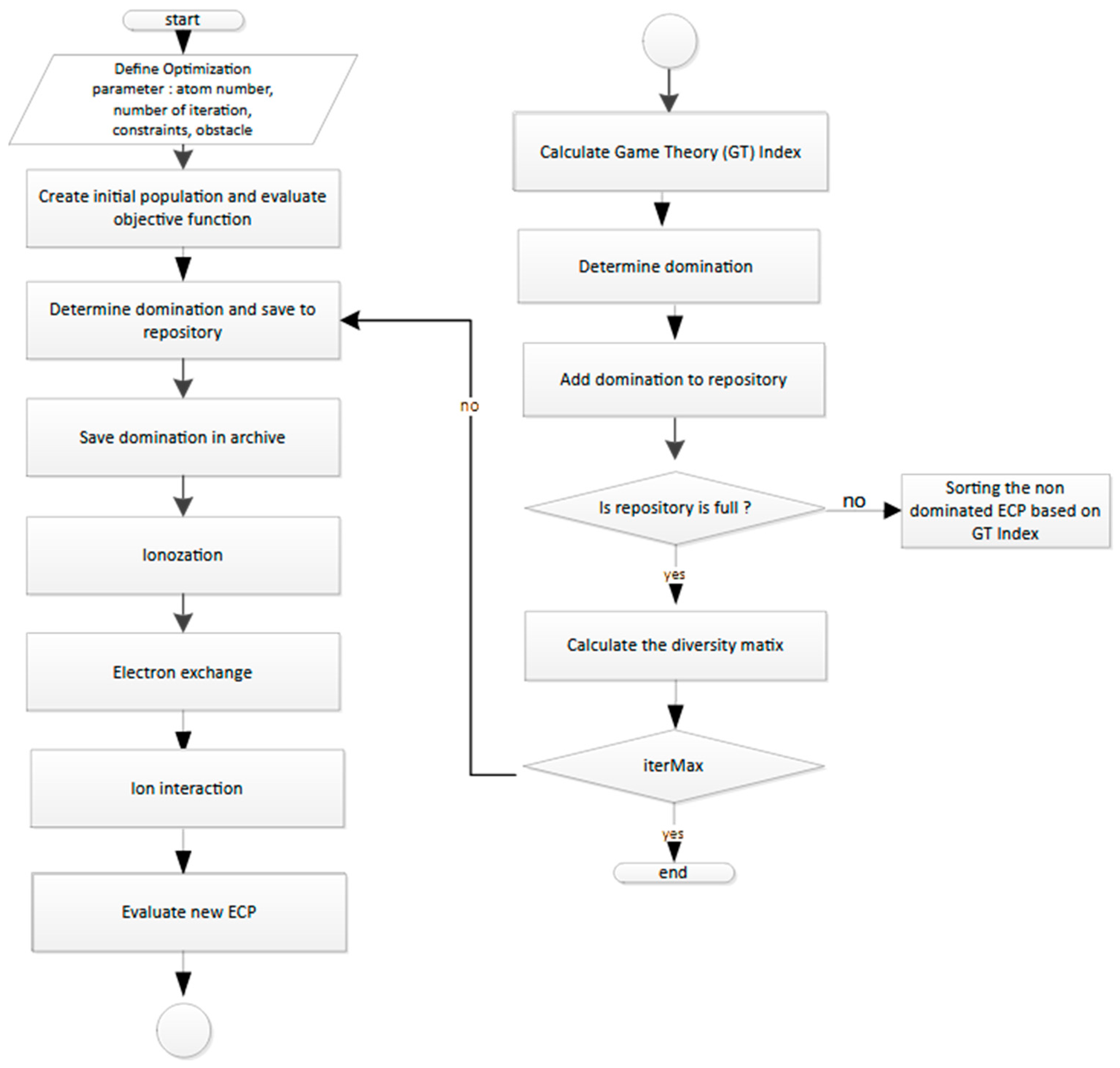
2.2. Research Flowchart
Figure 1 illustrates the comprehensive design methodology employed in this study. Broadly, the study encompasses two principal phases: assessment and optimization. The assessment phase involved the analysis of geographical and meteorological data obtained from the designated sites. These raw datasets underwent refinement through the WAsP map editor and WAsP climate analysis tools, culminating in the creation of the terrain and landscape maps alongside generalized wind speed data. Subsequently, leveraging WAsP CFD, these refined datasets were synthesized to produce a detailed wind resource map, accounting for the site’s specific wind and land characteristics.
The subsequent optimization phase was pivotal in designing the wind farm layout. The wind farm data, wind resource data, and WT specifications were modeled using Matlab software R 2023a. These inputs were then utilized to compute key objectives such as the LCOE and noise level for each potential wind farm configuration. The optimization process was executed through the MOMECPO algorithm, which iteratively refined the wind farm layout, meticulously considering all pertinent constraints to determine the optimal configuration.
2.3. Wind Turbine Model
The Vestas 2M turbine model was used as the wind turbine in this research. The WT parameter is shown in
Table 1, while the power curve is depicted in
Figure 2.
2.4. Wake Effect Model
The wake effect, which involves a decrease in wind speed and power following energy extraction by a turbine, presents a notable challenge in large wind farms, possibly reducing each turbine’s efficiency by up to 15% of the total power produced [
35]. Tackling this issue becomes a main goal in wind farm planning, emphasizing the importance of minimizing the wake effect. Strategic positioning of turbines to minimize the wake effect is important to achieve this goal to alleviate the adverse effects of power loss on nearby turbines.
Developing a model to simulate the wake effect in complex terrains presents a challenge due to the intricate relationship between terrain features and wake dynamics. Various research efforts have suggested approaches to estimate the wake effect in such environments. For example, a virtual particle wake model customized for intricate terrains within wind farms was proposed in ref. [
14,
36]. Moreover, ref. [
8,
31] enhanced the Jensen wake model, integrating the wind data acquired from the simulation of WAsP CFD.
In this research, the models outlined in [
12] and [
10] were adapted to model the wake effect by including terrain influences across all sites. The terrain flow data acquired from the simulation of WAsP CFD were merged with the Jensen wake model. In this model, the expansion of the wake from the upwind turbine to the downwind turbine was assumed to follow the terrain surface curve.
Figure 3 depicts the wake expansion between two WTs located at different elevations, (
xi,
yi) and (
xj,
yj). Wind travel from WT
i to WT
j encountered varying local wind speeds because of the influence of the terrain characteristic, with wind speeds denoted as
vi and
vj at WT
i and WT
j, respectively. The wind speed characteristics at both WTs are represented using the Weibull distributions denoted as (
ki,
ci,
θi) and (
kj,
cj,
θj), where k and c are the Weibull distribution’s shape and scale parameters, respectively.
The wake area expanded linearly with the increasing distance between the upwind and downwind turbines. At a distance
dyij, the radius of the wake is computed as
rw = kdyij + ri, where k denotes the coefficient of wake expansion that depends on the WT hub height and the surface roughness index
Zo. The wake from the upwind turbine WT
i affects the decreasing of the wind speed
vj at the downwind turbine WT
j following Equation (5), where
CT is the thrust coefficient of WT.
For a wind farm, the wake areas between upstream and downstream WTs depend on their hub height, rotor diameters, and the changes in the wind direction. The wake areas
As can be calculated by using Equation (6).
The wake regions between the upstream and downstream WTs are influenced by factors such as their WT hub height, rotor diameters, and alterations in wind direction. These wake areas, denoted as A
s, are determined through Equation (7).
The downwind WT will be influenced by upwind WT if and only if
where
2.5. LCOE Model
Wind speed and direction distribution play a crucial role in shaping the energy production of a wind farm. This study employed the Weibull distribution to characterize the wind distribution. The expected energy production from a WT was then calculated using Equation (11) [
37].
The cost per kWh of energy conversion from the wind, denoted as COE [USD per kWh], represents the threshold at which the wind farm’s operation throughout its operational life neither generates economic profits nor incurs losses [
24]. The concept of levelized COE (LCOE) is similar to COE, with the vital distinction being that LCOE accounts for the separation of fixed and variable costs. LCOE incorporates the temporal aspect of monetary value, factoring in variables such as interest and inflation rates. It is closely tied to the life cycle cost, a relationship that can be mathematically modeled using Equation (12).
CAPEX includes turbine, installation, foundation, and transmission costs. Depending on their specifications, turbines represent 75% to 85% of this [
38]. Foundation costs vary with soil structure, while installation costs are tied to the foundation type. Transmission costs generally contribute 2% to 15% of total CAPEX [
39]. OPEX can be a fixed value, a percentage of other costs, or a function based on annual expenses. It typically covers tools, labor, and decommissioning costs, which can be 1.2 to 2.5 times the project’s total investment [
40,
41]. The capital recovery factor (CRF) calculates the annual cost for a project, taking into account the interest rate (i) and the project’s lifespan (N) in the CRF formula (Equation (13)).
This research used the mass-based model developed by the National Renewable Energy Laboratory (NREL) to calculate CAPEX and OPEX [
41]. The calibration of the wind farm cost was based on a report by NREL [
2] and from ref. [
42]. The land type was considered the cost component, including land acquisition, compensation payment for farmers, and land clearing costs. The acquisition cost and compensation of the farming area were based on the report of the Sidrap wind farm project [
43], and the land clearing cost was based on ref. [
44].
2.6. Noise Model
In our study, we performed thorough noise calculations along the boundaries of each site as the selecting points where the noise level was calculated. The average noise level in all these points was used as the objective to minimize. Following the ISO-9613-2 standard [
21], we evaluated sound pressure levels (SPLs) across eight frequency octaves at each noise receptor. This assessment was conducted by determining the sound power in each octave band for each noise source, covering frequencies from 63 Hz to 8 kHz using Equation (14). The equation includes factors such as directivity correction (
Dc), octave band attenuation (
A), and indexing for each frequency octave (
f).
The attenuation term
A is expressed in the following Equation (15):
The contribution of each sound source at each octave band was summed to ascertain the weighted downwind sound pressure level at a particular location. A-weighted sound pressure levels (SPLs) are commonly employed in wind farm layout applications [
45]. The collective contributions from each point source across all octave bands can be employed to calculate the continuous A-weighted SPL downwind at a specified position.
In Equation (16), represents the number of sound sources, j is the index corresponding to each of the eight standards octave-band mid-band frequencies, and represents the standard A-weighting coefficient for a given frequency band.
In multiobjective optimization, turbine placement and operational settings are the primary design variables influencing noise reduction. Optimizing the turbine layout (location and spacing) directly impacts Dc, as greater distances can help lower Lf. Additionally, adjustments to turbine parameters (such as rotational speed) can reduce Lw, the initial noise emitted by each turbine.
By systematically balancing these design variables, multiobjective optimization algorithms can explore tradeoff solutions where the layout minimizes both noise levels and the LCOE, presenting planners with optimal configurations that meet both economic and environmental goals.
2.7. Land Characteristic Model
This research tackled two critical challenges in optimizing wind farm layouts: the slope index and land cover considerations. The slope index significantly impacts wind farm development costs, particularly when installing WTs on steep slopes. As slopes steepen, land modification for level turbine foundations becomes necessary. The cost of reshaping the land relates to the area required for each turbine’s foundation, as defined in Equation (17). Assuming the land cut takes a rectangular shape with the WT diameter as its side, the cost is USD 10 per 1 m
3. As the number of turbines on steeper slopes increases, so do the costs, thereby elevating the LCOE.
Land cover significantly affects both energy production and wind farm costs.
Table 2 presents the varied roughness index for distinct land cover types. The roughness index (
z0) on each land cover and the hub height of the WT will influence the wake expansion (
k) coefficient that will further affect the energy produced by a WT, as shown in Equation (18).
Different land cover types also significantly affect wind farm costs. The agricultural land occupation involves costs like land acquisition and farmer compensation, while forest land occupation necessitates land clearing and leveling expenses. Additionally, residential zones are typically restricted in wind farm layout design. Detailed cost considerations for each land cover type are outlined in
Table 3.
4. Result and Discussion
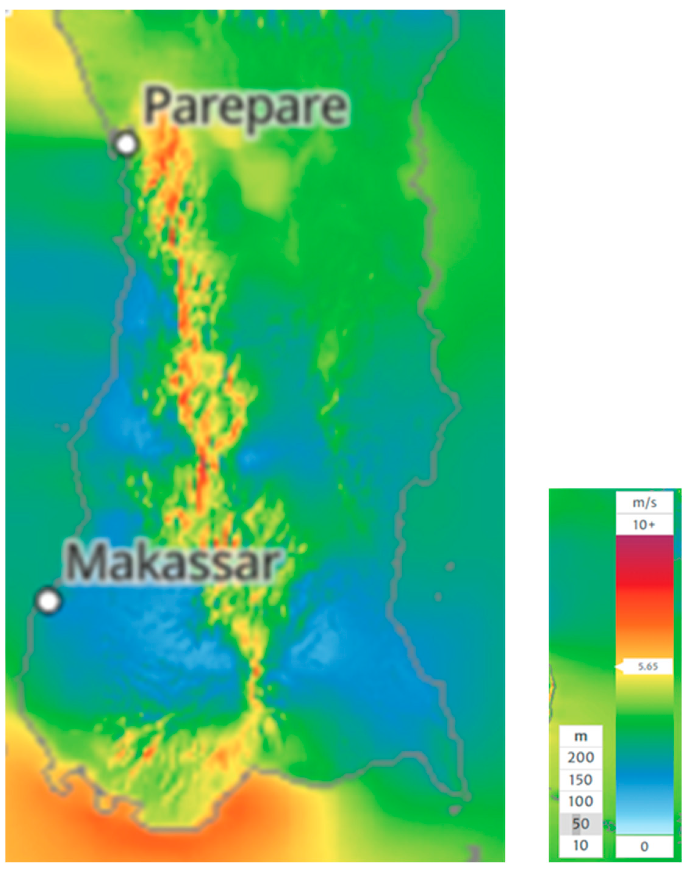
4.1. Wind Farm Site Selection
In this study, three sites with distinct terrain types—flat terrain, semi-complex terrain, and complex terrain—were selected, all located in South Sulawesi, Indonesia. Selecting an appropriate site for a wind farm involves a comprehensive evaluation of various criteria, primarily focusing on factors such as wind speed and terrain type. The initial step in the selection process was the identification of wind power potential maps for the assessment areas.
A Global Wind Atlas (GWA) map [
50] was used in this process, providing mean wind speed data to access the area with a high potential for wind energy generation.
Figure 6 illustrates the wind power potential map for the selected assessment areas at 50 m in height.
Wind power potential is classified into seven classes based on mean wind speed. Geospatial information system (GIS) applications are used to extract maps with these classifications. In this study, mean wind speed was the primary indicator to identify areas on the map with wind power classes that met or exceeded a specified threshold. Class 2, with 5.6 m/s as a lower wind speed boundary, was used as the lower limit in this study, and the area with a wind power class lower than class 2 would be removed.
Figure 7 highlights the areas with a wind power class that was the same or more than class 2.
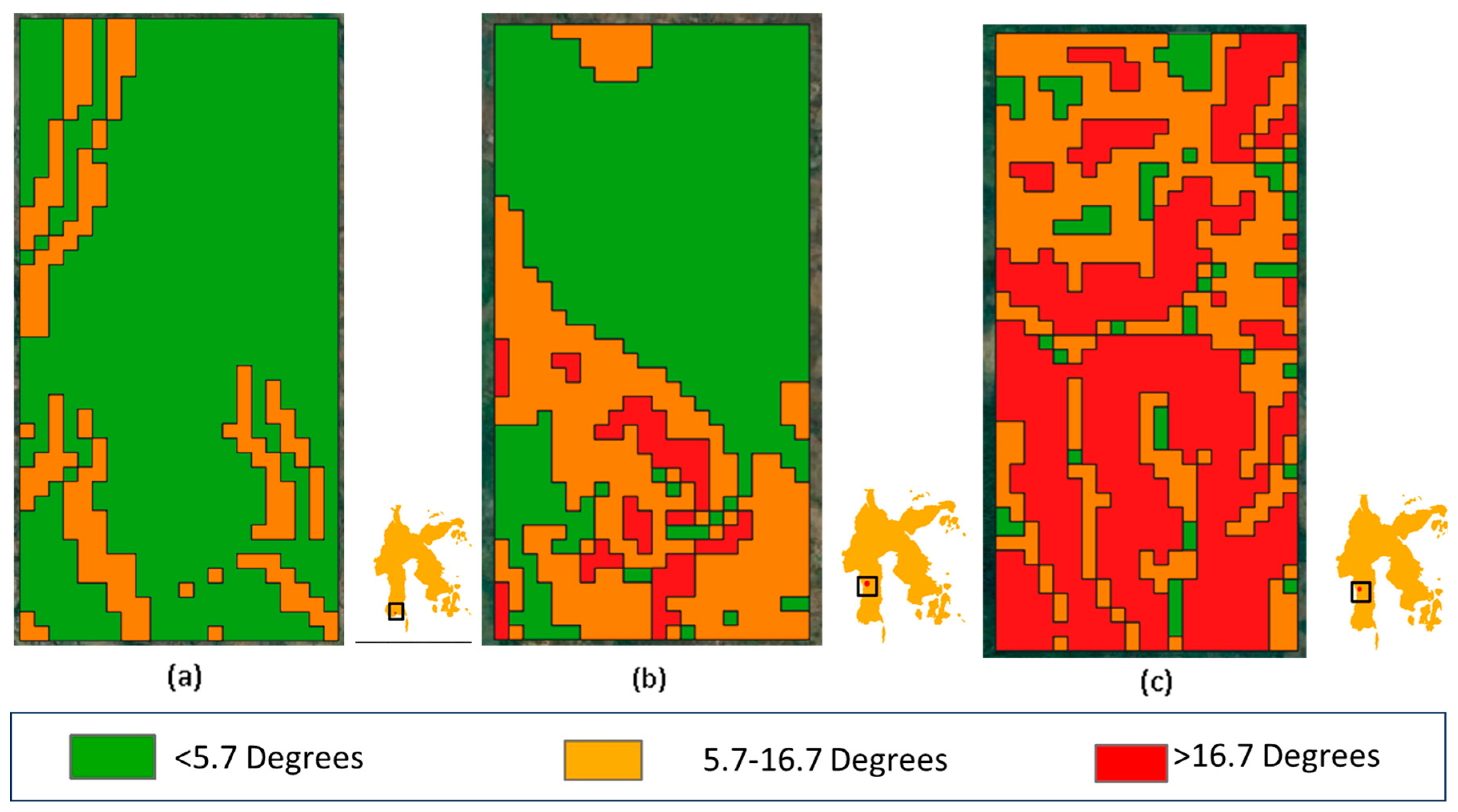
The next step in the selection process involved evaluating the terrain type, with slope degree as the primary indicator for classification. The slope map was analyzed by identifying areas from
Figure 8 using two slope thresholds, which were 5.7 and 16.7 degrees. The area was classified into three parts: below 5.7 degrees, from 5.7 to 16.7 degrees, and above 16.7 degrees.
Figure 8 displays the map of areas with a wind power class above class 2 with three parts of slope areas differentiated by two slope thresholds. The map shows that flat terrain was predominantly located in the southern part of the area, while semi-complex and complex terrain were mainly found in the middle and northern parts. Therefore, the area in the southern part was selected for flat terrain location, while the northern part was chosen for the semi-complex and complex terrain locations due to the availability of a larger area.
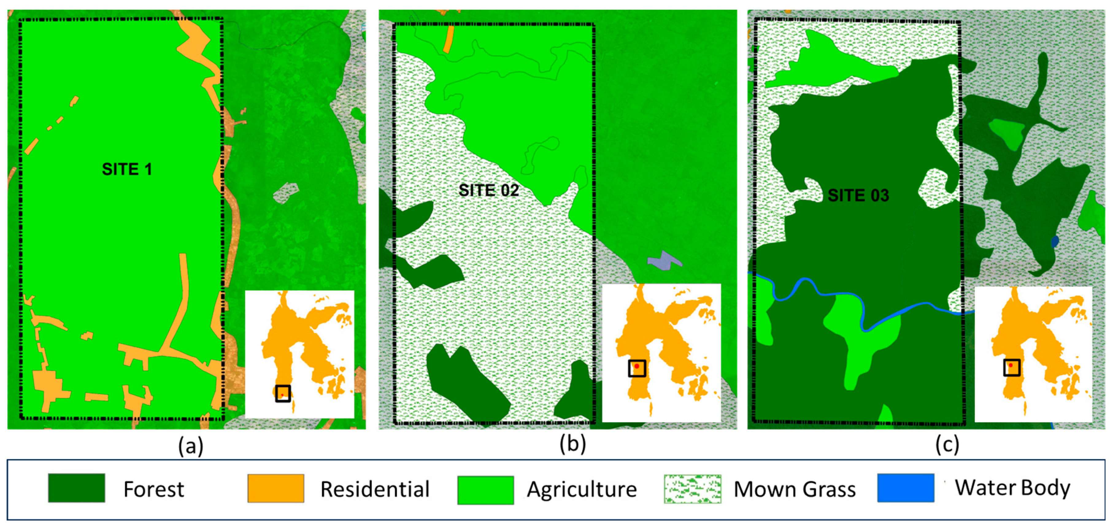
Sites of identical size but with varying terrain types were selected from the investigated locations. Each site had a rectangular shape, measuring 4 km in length and 2 km in width, and was designated as Site 1, Site 2, and Site 3. The terrain type for each site was classified based on its ruggedness index (RIX). Site 1, located in the southern part of the area, was categorized as flat terrain, while Site 2 and Site 3, situated in the northern part, were classified as semi-complex and complex terrains, respectively. This study focused on designing and planning wind farms at these three sites, as no prior wind farms had been developed in these areas.
Table 4 presents the RIX values for each site.
Figure 9 and
Figure 10 visually depict the boundaries of each site processing by using QGIS 3.28.0 software. As illustrated in the figures, the rectangular boundary lines serve as construction boundaries, ensuring optimal placement for the WTs. The terrain characteristics of the designated sites are illustrated in
Figure 9. The slope data were analyzed from the digital elevation model (DEM) obtained from the Global 30 Arc-Second Elevation (GTOPO30) dataset [
51]. The sites were divided into three slope ranges: less than 5.7 degrees, from 5.7 to 16.7 degrees, and more than 16.7 degrees. Within this representation, it was evident that Site 1 exhibited relatively flat terrain, with most areas having slopes less than 5.7 degrees. In contrast, Site 2 features semi-complex terrain, predominantly comprising areas with slopes below 16.7 degrees. Meanwhile, Site 3 was classified as complex terrain, with most regions having slopes exceeding 16.7 degrees.
Figure 10 provides a detailed insight into the landscape characteristics of the three sites. The land cover map was obtained from global land cover characterization (GLCC) by the U.S. Geological Survey [
52]. The figure shows that Site 1 is predominantly marked by farmland with an open appearance, interspersed with residential areas. Site 2 primarily comprises mown grass, with approximately one-third of certain regions designated for farmland and a few areas covered by forests.
Site 3 is predominantly forested, with limited sections featuring mown grass and farmland. Forested terrain generally has a high roughness length (Z0) due to trees and vegetation. To reach more consistent winds above the tree canopy, turbines in these areas often require taller towers, typically over 100 m. This adds to installation costs and engineering complexity, but the height enables turbines to capture stronger, steadier winds. Advanced turbine technology, designed to perform in turbulent conditions, can also help optimize energy capture in these areas. Careful wind resource assessments are essential to determine ideal turbine placement.
Environmentally, forested areas are often biodiverse, meaning that installation must account for potential impacts on wildlife, habitats, and ecosystems. Environmental impact assessments (EIAs) and strict regulations are typically required, with efforts to minimize deforestation and mitigate habitat disruption. While the higher costs and environmental considerations may be challenging, forested wind farms can still be economically viable, especially in regions with strong renewable energy demand or government incentives. Careful planning and investment make wind energy development in forested areas possible, albeit with more complexities than open terrain projects.
4.2. Optimization Result
This study used the MOMECPO algorithm to optimize wind farm layouts across three distinct terrains. An extensive evaluation compared the MOMECPO performance with eight other algorithms in the same setting of population size, iterations, and archive size, and each algorithm was simulated through eight trial runs simultaneously. Performance assessment relied on two key indicators: RNI and hypervolume.
In practical wind farm design, achieving a singular ‘optimal solution’ is crucial. This research presents two tradeoff solutions: the LCOE tradeoff and the noise tradeoff. The LCOE tradeoff represents the point on the Pareto front with the lowest LCOE value, while the noise tradeoff represents the point with the lowest noise level. These tradeoff solutions allowed a comparative assessment of MOMECPO performance in minimizing each objective function. Moreover, another solution called the best compromise result was presented to depict the wind farm layout in the corresponding terrain and landscape map. This result is a point in the Pareto front with the highest distance of hypervolume, indicating the balancing between the LCOE and noise level.
4.2.1. Site 1
Site 1 features mostly flat terrain below a 5.7-degree slope, consisting of farmland with an open appearance and residential zones. The penalty value was applied to the layout if a WT was located in residential zones, while additional cost was added if a WT was located in the farmland. With 14 residential and 36 farmland grids, this site is crucial in assessing algorithms to avoid local optima and eliminate forbidden grids. Algorithms with low diversity struggle to avoid these grids, as evidenced by three out of nine algorithms—MOJAYA, MOEAD, and PESA2—failing to eliminate penalty values from the Pareto front even after 200 iterations.
Table 5 compares the proposed MOMECPO algorithm with eight other algorithms, highlighting MOMECPO’s consistently superior performance, particularly in achieving lower LCOE and noise levels across both tradeoff solutions. Specifically, MOMECPO effectively minimized LCOE to 6.7855 US cents/kWh and reduced noise to 53.7069 dB. The algorithm excelled in both exploration and exploitation of the Pareto front. Its exploration capability was demonstrated by generating an average of 32 non-dominated solutions, which was higher than other algorithms, as illustrated in
Figure 11. The exploitation strength was evident from the location of these non-dominated solutions, predominantly found in the lower-left quadrant. The detailed multiobjective evaluation in
Table 6 further emphasizes MOMECPO’s superiority, with the highest RNI indicating enhanced exploration and the highest hypervolume reflecting strong exploitation, establishing MOMECPO as a leading algorithm among its peers.
Figure 12 displays the best compromise wind farm layout for Site 1: a grid layout on the upper left side demonstrates power generated (red numbers), power losses due to the wake effect (green numbers), additional costs related to land features (blue numbers), and noise levels (purple numbers), while the above section shows the WT position related to the site’s landscape and terrain characteristics. The layout shows that all the WTs located in farmland area with lower degree slopes (<5.7 degrees).
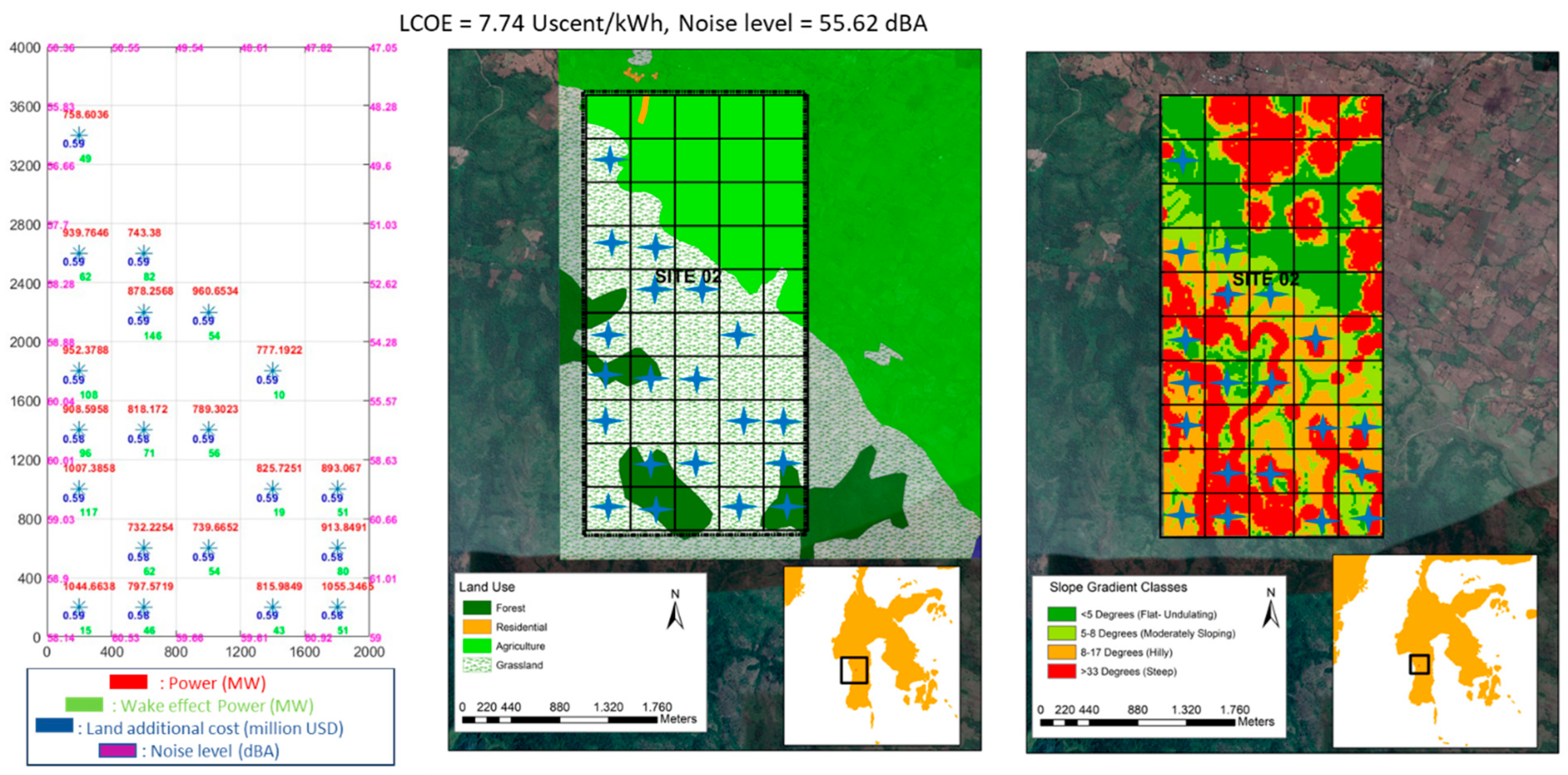
4.2.2. Site 2
Site 2 features a diverse landscape encompassing farmland, grassland, forest, and a residential grid. This site was characterized as a semi-complex terrain, with 8% of the land having a slope higher than 16.7 degrees. This site consists of only one residential grid that is set as restricted, while WTs can occupy 49 grids. This condition increases the number of non-dominated solutions. Therefore, sorting was important to sort the quality of the obtained non-dominated solution. For this purpose, game theory sorting played a crucial role by removing solutions with a lower game theory index to enhance the solution diversity.
Table 7 summarizes the results for Site 2, highlighting MOMECPO’s superior performance on LCOE level results compared with all the other algorithms and with competitive noise slightly lower than the NSGAIII.
On average, the MOMECPO algorithm generated a set of 50 non-dominated solutions.
Figure 13 visually shows the Pareto front yielded for the MOECPO and other compared algorithms. MOMECPO can produce 50 non-dominated solutions located in the lower-left quadrant of the chart, demonstrating the algorithm’s ability to generate diverse results efficiently. This result underscores MOMECPO’s superiority in addressing the unique challenges presented by this site.
Table 8 provides a detailed summary of performance indicators for various multiobjective algorithms, revealing MOMECPO as the standout performer. It consistently delivered a more significant number of non-dominated solutions, reflected in its highest RNI score, signifying an exceptional exploration quality. Moreover, MOMECPO achieved the highest hypervolume value among all the algorithms, indicating superior exploitation quality.
Figure 14 depicts the best compromise wind farm layout for Site 2. All turbines were placed within grids containing grassland and forest, influenced significantly by the cost function, preferring grassland over farmland. Furthermore, WTs predominantly occupy the southwest regions with higher wind speeds and slopes.
4.2.3. Site 3
Site 3 features a complex terrain characteristic, with 55% of the land having a slope higher than 16.7 degrees. This site is covered predominantly by forest across 36 grids. Additionally, it includes areas designated for bare soil, farmland, and grassland, while five grids along riverbanks prohibit WT installations. Site 3 has higher wind velocity, promising increased annual energy yield but requiring additional costs due to the rugged, steep terrain. This unique environment presents both opportunities and challenges for wind energy utilization.
Table 9 shows the tradeoff solution for Site 3. Due to the higher wind speed generating more energy, Site 3 exhibits a lower LCOE than the previous sites. MOMECPO achieves the lowest LCOE in the tradeoff result and the second-lowest noise level in the noise tradeoff after the NSGAII.
MOMECPO yielded around 20 solutions at this site, concentrated in the lower-left quadrant of
Figure 15, similar to previous sites.
Table 10 outlines how MOMECPO achieved the best performance at Site 3. It outperformed other algorithms in exploiting and exploring the Pareto front, with the highest RNI score and hypervolume. This positions MOMECPO as the leader, presenting diverse solutions while attaining top-tier results at Site 3.
Figure 16 depicts the best compromise wind farm layout for Site 3. Most WTs (17 WT) are located in forested areas on this site. Only two turbines are in grassland and one in farmland regions.
4.3. Analysis of the Effect of Terrain and Landscape Characteristic
Each site examined in this study exhibits different terrain and landscape characteristics. Site 1, characterized by flat terrain, predominantly comprises agricultural areas featuring a mediated value roughness length (Z0 = 0.05). Site 2, predominantly grassland, is categorized as semi-complex terrain with a notably lower roughness length of approximately 0.008. In contrast, Site 3 is classified as a complex terrain with elevated topography.
Table 11 shows the comparison of the AEP at each site. The analysis of environmental parameters Z
0 and RIX on the AEP at three sites reveals interesting insights into how these factors influence energy output. Site 1, with a RIX of 0% and a Z
0 of 0.05, shows relatively low roughness, which typically results in higher wind speeds. Despite this, its gross AEP is lower than Site 3, which has the highest RIX (55%) and a considerably higher Z
0 of 0.8, indicating a much rougher terrain. This roughness at Site 3, however, appears to correspond to high wind resource availability, giving it the highest gross AEP at 301.391 GWh. Site 2, with a RIX of 8% and a lower Z
0 of 0.008, exhibits a smaller gross AEP (236.956 GWh) and the highest wake effect (19.6 GWh), which further impacts its net AEP.
In terms of wake effect, Site 3 benefits from the lowest wake-effect losses (9.44 GWh), attributed to higher roughness length. Consequently, Site 3 achieves the highest net AEP (291.949 GWh) even with rougher terrain. Site 1 has a higher net AEP than Site 2, despite Site 2’s lower roughness, highlighting that higher wake losses can offset the benefits of reduced terrain roughness. This analysis suggests that while rougher terrain can correlate with increased wind resources (as in Site 3), it can also necessitate careful management of turbine positioning to minimize wake effects and maximize net energy output.
Table 12 presents data on three sites, focusing on the tradeoffs between LCOE and noise levels. For the LCOE tradeoff, Site 1 has a mean LCOE of 6.785 US cents/kWh with a noise level of 55.891 dBA. Site 2 has a slightly higher LCOE mean at 7.729 US cents/kWh, with a noise level of 55.763 dBA. Site 3 has the lowest LCOE at 5.561 US cents/kWh but with the highest noise level at 56.919 dBA. In the noise tradeoff, Site 1 achieves a lower noise level of 53.705 dBA but with an increase in LCOE to 7.66 US cents/kWh. Site 2 reaches the lowest noise at 52.529 dBA but with the highest LCOE at 9.719 US cents/kWh. Site 3 maintains a balanced approach, achieving a mean LCOE of 5.811 US cents/kWh with a noise level of 55.253 dBA.
Site 3 also produces the lowest LCOE compared with the other sites due to the higher energy produced in this site. Regarding the noise level, higher AEP also impacts higher noise levels attributed to its terrain characteristics, specifically Z0 and RIX. Site 3 has a high Z0 value of 0.8, indicating significant surface roughness due to obstacles like hills or vegetation, which create turbulence in the airflow. This turbulence helps enhance wind mixing and provides a more consistent wind flow at the turbine’s hub height, leading to increased energy production and thus a lower LCOE. However, this same turbulent airflow also generates additional aerodynamic noise, as the turbine blades encounter fluctuating wind speeds and directions, increasing blade–vortex interactions and resulting in more noise. Additionally, the high RIX value of 55% suggests that Site 3 has steep and rugged terrain. The elevation changes associated with a high RIX cause further fluctuations in wind speeds as the air moves over the uneven terrain, resulting in unsteady aerodynamic loads on the blades. These loads create noise through mechanisms like vortex shedding and flow separation. While these rugged conditions allow for efficient energy capture and a lower LCOE, they also lead to higher noise levels due to the turbulent wind environment. Thus, Site 3’s terrain properties illustrate the tradeoff between low energy costs and increased noise in areas with high roughness and ruggedness.
For future site planning, a balanced approach is recommended, one that weighs the benefits of higher wind speeds against the challenges of roughness-induced turbulence and wake effects. Conducting a correlation analysis between RIX and Z0 would quantify these relationships further. Additionally, a comparative study of different turbine models across varying environmental conditions, alongside long-term monitoring, could provide insights into optimizing wind farm performance amidst changing environmental parameters.


 ,
, 


