
Multi-Objective Optimal Integration of Distributed Generators into Distribution Networks Incorporated with Plug-In Electric Vehicles Using Walrus Optimization Algorithm

 and
and 
Abstract
1. Introduction
- It is the first time to apply the recently developed WO approach to determine the near-optimal locations and ratings of DGs in RDNs incorporated with PEVs;
- Two standard 33-bus and 69-bus RDNs beside one real distribution system of ShC-D8 in Egypt are analyzed, considering a time-varying voltage-dependent load model;
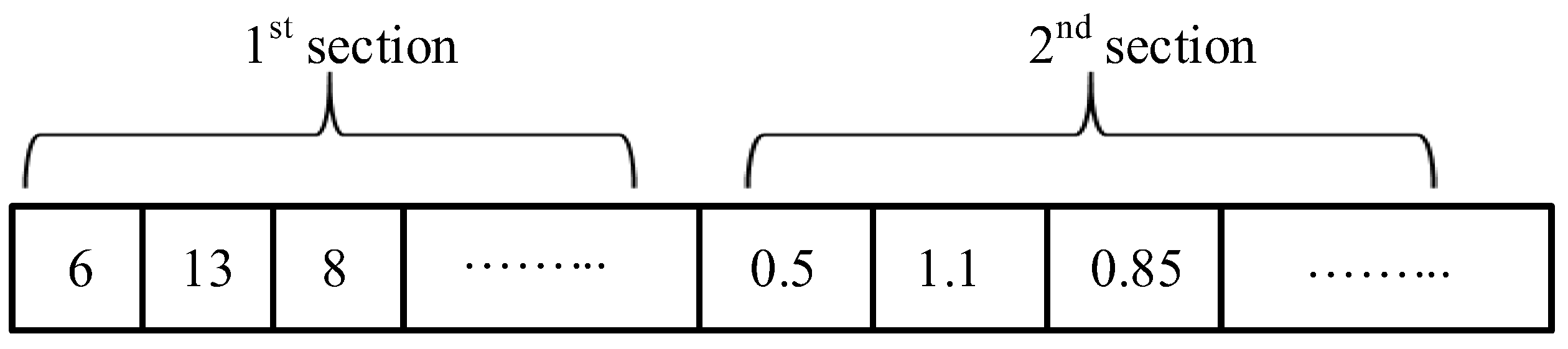
- Two types of DGs, with unity and non-unity power factors, are used in this study while adapting WO so that the first decision variables must be integer numbers representing DGs’ locations and the others represent DGs’ ratings and power factors;
- Constraints like power balance, buses’ voltages, and line flow are taken into consideration in the optimization model to present a more realistic problem;
- The efficacy and superiority of the proposed WO are verified by comparing it to other approaches.
2. Distribution Network Modelling Framework
2.1. DG Modelling
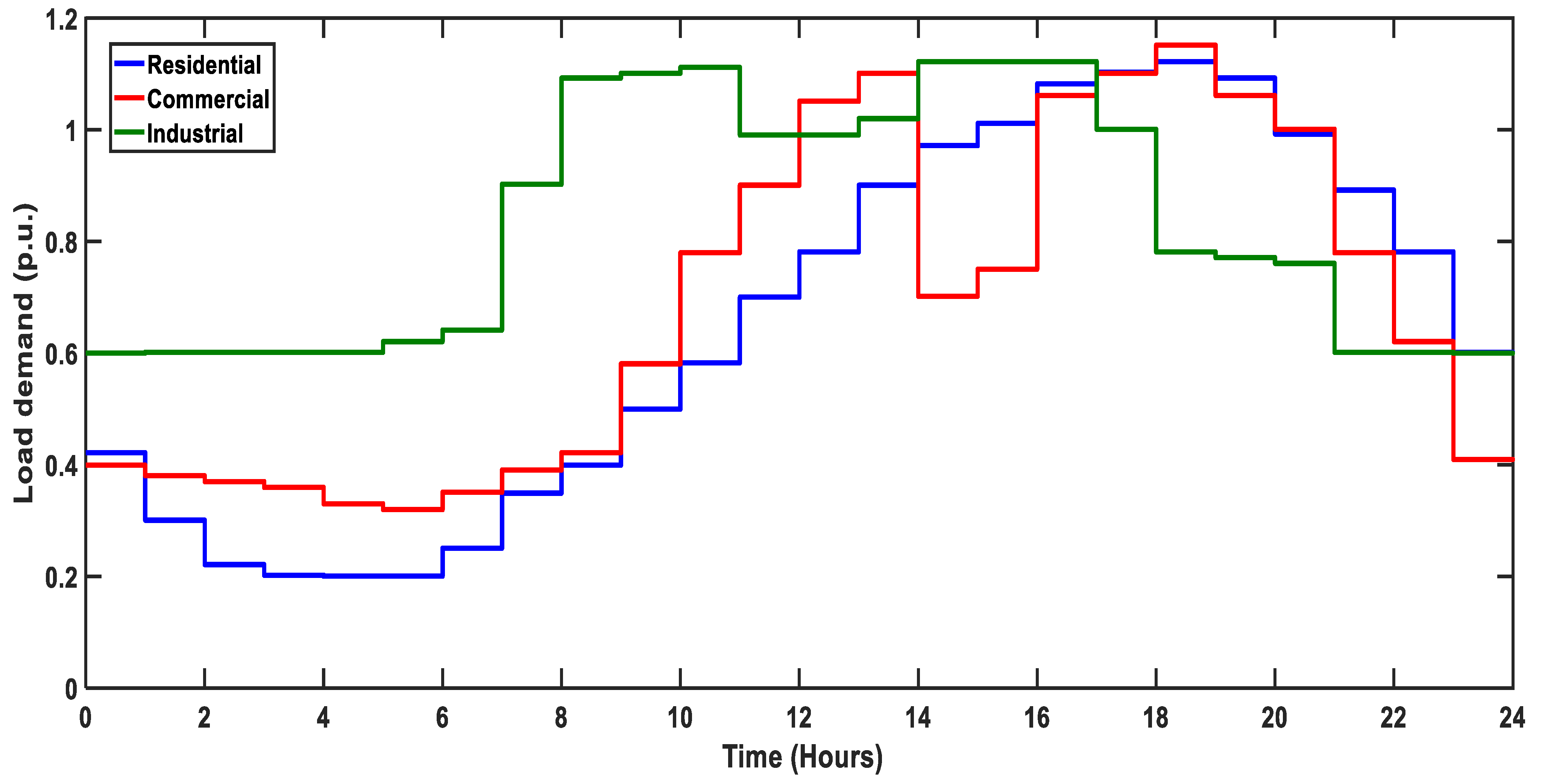
2.2. Load Modelling
2.3. Load Flow Model
2.4. Objective Function
2.4.1. Power Loss Index (PLI)
2.4.2. Voltage Stability Index (VSI)
2.4.3. Voltage Deviation Index (VDI)
2.5. Constraints
2.5.1. Power Balance Constraints
2.5.2. Bus Voltage Constraints
2.5.3. Sizing Limits of DGs
2.5.4. Line Flow Constraints
2.5.5. Treatment of Constraints
3. The WO Approach
3.1. General Overview
3.2. Mathematical Model of WO
3.2.1. Phase (1): Initialization
3.2.2. Phase (2): Giving Danger and Safety Signals
3.2.3. Phase (3): Migration (Exploration)
3.2.4. Phase (4): Reproduction (Exploitation)
Roosting Behavior
Foraging Behavior
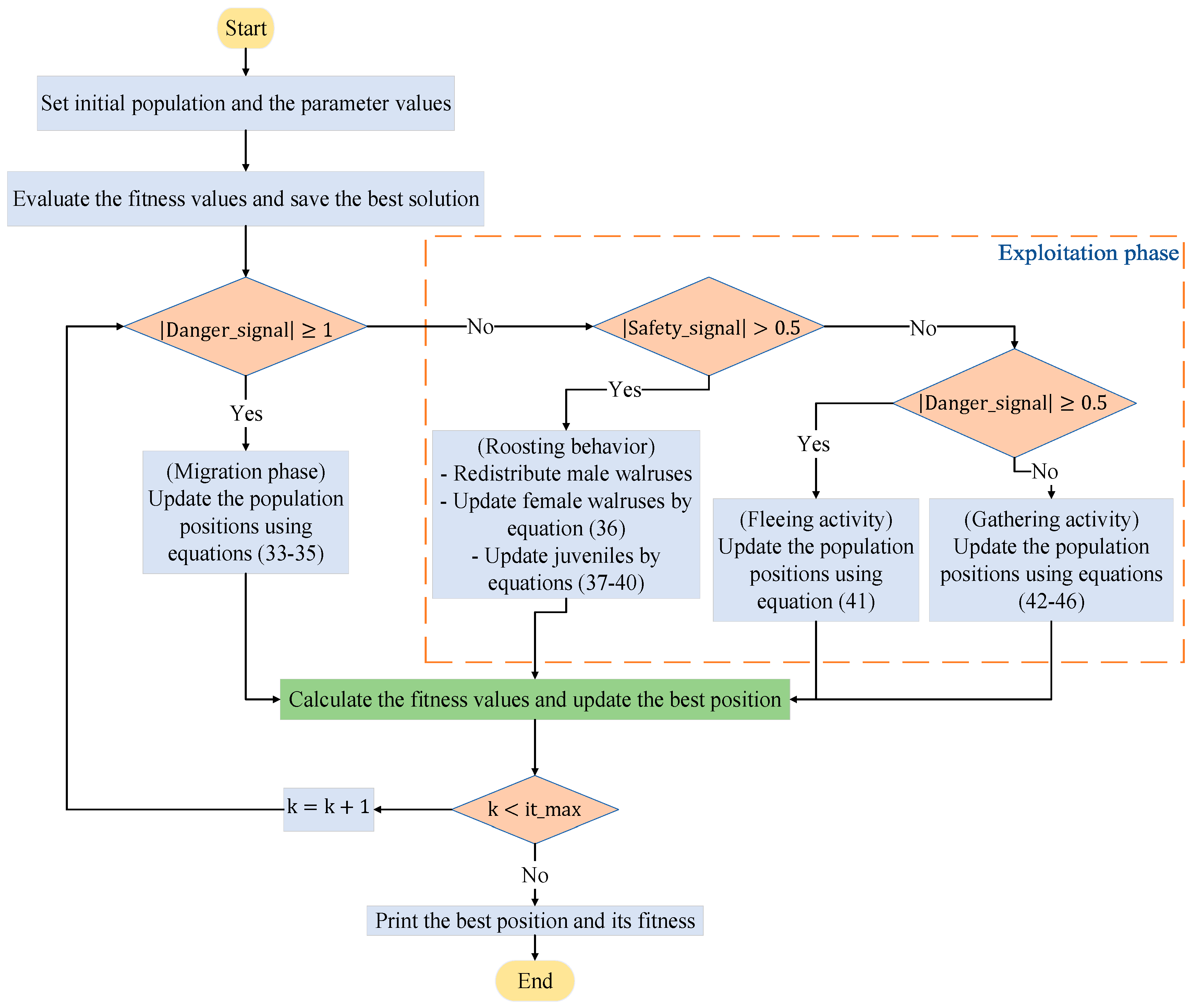
3.3. Procedures of WO
3.4. Application of WO Approach on the DG Allocation Problem
4. Results and Discussions
- Case 0: Without PEVs and DG units;
- Case 1: With PEVs under the PC scenario and without DG units;
- Case 2: With PEVs under the OPC scenario and without DG units;
- Case 3: Optimal allocation of unity power factor DGs in the presence of PEVs under a PC scenario;
- Case 4: Optimal allocation of non-unity power factor DGs in the presence of PEVs under a PC scenario.
4.1. PEV Charging Demand
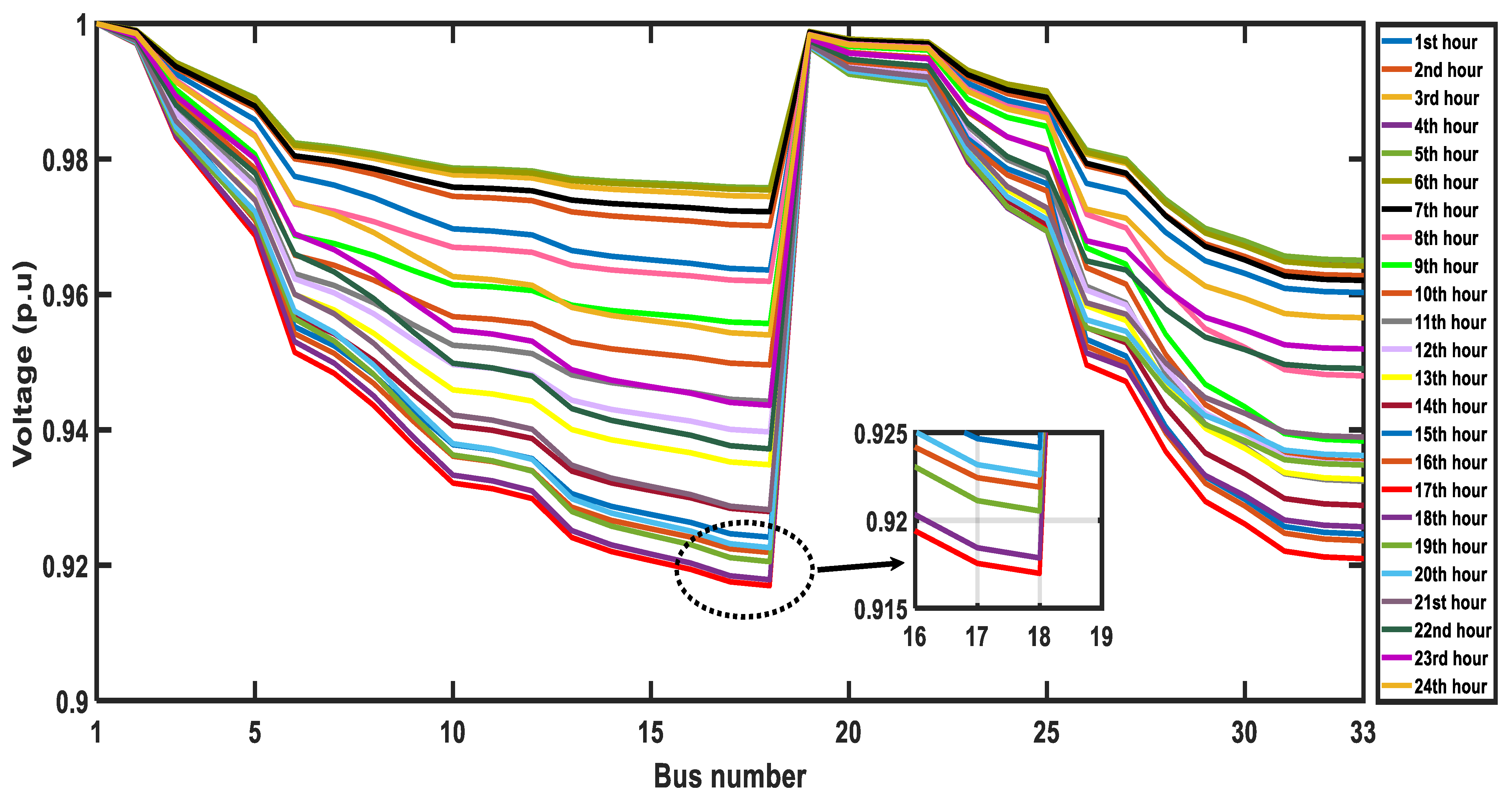
4.2. IEEE 33-Bus System
4.3. IEEE 69-Bus System
4.4. ShC-D8 System in Egypt
5. Conclusions
Author Contributions
Funding
Institutional Review Board Statement
Informed Consent Statement
Data Availability Statement
Conflicts of Interest
References
- Zeb, M.Z.; Imran, A. Optimal placement of electric vehicle charging stations in the active distribution network. IEEE Access 2020, 8, 68124–68134. [Google Scholar] [CrossRef]
- Yuvaraj, T.; Devabalaji, K.; Thanikanti, S.B.; Aljafari, B.; Nwulu, N. Minimizing the electric vehicle charging stations impact in the distribution networks by simultaneous allocation of DG and DSTATCOM with considering uncertainty in load. Energy Rep. 2023, 10, 1796–1817. [Google Scholar]
- Shareef, H.; Islam, M.M.; Mohamed, A. A review of the stage-of-the-art charging technologies, placement methodologies, and impacts of electric vehicles. Renew. Sustain. Energy Rev. 2016, 64, 403–420. [Google Scholar] [CrossRef]
- Das, H.S.; Rahman, M.M.; Li, S.; Tan, C.W. Electric vehicles standards, charging infrastructure, and impact on grid integration: A technological review. Renew. Sustain. Energy Rev. 2020, 120, 109618. [Google Scholar] [CrossRef]
- Alquthami, T.; Alsubaie, A.; Alkhraijah, M.; Alqahtani, K.; Alshahrani, S.; Anwar, M. Investigating the impact of electric vehicles demand on the distribution network. Energies 2022, 15, 1180. [Google Scholar] [CrossRef]
- Roy, P.; Ilka, R.; He, J.; Liao, Y.; Cramer, A.M.; Mccann, J.; Delay, S.; Coley, S.; Geraghty, M.; Dahal, S. Impact of electric vehicle charging on power distribution systems: A case study of the grid in western kentucky. IEEE Access 2023, 11, 49002–49023. [Google Scholar] [CrossRef]
- Hussan, U.; Majeed, M.A.; Asghar, F.; Waleed, A.; Khan, A.; Javed, M.R. Fuzzy logic-based voltage regulation of hybrid energy storage system in hybrid electric vehicles. Electr. Eng. 2022, 104, 485–495. [Google Scholar] [CrossRef]
- Sellami, R.; Farooq, S.; Rafik, N. An improved MOPSO algorithm for optimal sizing & placement of distributed generation: A case study of the Tunisian offshore distribution network (ASHTART). Energy Rep. 2022, 8, 6960–6975. [Google Scholar]
- Truong, K.H.; Nallagownden, P.; Elamvazuthi, I.; Vo, D.N. A quasi-oppositional-chaotic symbiotic organisms search algorithm for optimal allocation of DG in radial distribution networks. Appl. Soft Comput. 2020, 88, 106067. [Google Scholar] [CrossRef]
- Abujubbeh, M.; Fahrioglu, M.; Al-Turjman, F. Power loss reduction and voltage enhancement via distributed photovoltaic generation: Case study in North Cyprus. Comput. Electr. Eng. 2021, 95, 107432. [Google Scholar] [CrossRef]
- Huy, P.D.; Ramachandaramurthy, V.K.; Yong, J.Y.; Tan, K.M.; Ekanayake, J.B. Optimal placement, sizing and power factor of distributed generation: A comprehensive study spanning from the planning stage to the operation stage. Energy 2020, 195, 117011. [Google Scholar] [CrossRef]
- Gao, H.; Diao, R.; Zhong, Y.; Zeng, R.; Wu, Q.; Jin, S. Optimal allocation of distributed generation in active distribution power network considering HELM-based stability index. Int. J. Electr. Power Energy Syst. 2024, 155, 109508. [Google Scholar] [CrossRef]
- Ayanlade, S.O.; Ariyo, F.K.; Jimoh, A.; Akindeji, K.T.; Adetunji, A.O.; Ogunwole, E.I.; Owolabi, D.E. Optimal allocation of photovoltaic distributed generations in radial distribution networks. Sustainability 2023, 15, 13933. [Google Scholar] [CrossRef]
- El-Fergany, A.A. Optimal capacitor allocations using evolutionary algorithms. IET Gener. Transm. Distrib. 2013, 7, 593–601. [Google Scholar] [CrossRef]
- Islam, M.R.; Lu, H.; Hossain, M.J.; Li, L. Mitigating unbalance using distributed network reconfiguration techniques in distributed power generation grids with services for electric vehicles: A review. J. Clean. Prod. 2019, 239, 117932. [Google Scholar] [CrossRef]
- Ghosh, S.; Ghoshal, S.P.; Ghosh, S. Optimal sizing and placement of distributed generation in a network system. Int. J. Electr. Power Energy Syst. 2010, 32, 849–856. [Google Scholar] [CrossRef]
- Hung, D.Q.; Mithulananthan, N. Multiple distributed generator placement in primary distribution networks for loss reduction. IEEE Trans. Ind. Electron. 2011, 60, 1700–1708. [Google Scholar] [CrossRef]
- Mahmoud, K.; Yorino, N.; Ahmed, A. Optimal distributed generation allocation in distribution systems for loss minimization. IEEE Trans. Power Syst. 2015, 31, 960–969. [Google Scholar] [CrossRef]
- Al Abri, R.S.; El-Saadany, E.F.; Atwa, Y.M. Optimal placement and sizing method to improve the voltage stability margin in a distribution system using distributed generation. IEEE Trans. Power Syst. 2012, 28, 326–334. [Google Scholar] [CrossRef]
- Rueda-Medina, A.C.; Franco, J.F.; Rider, M.J.; Padilha-Feltrin, A.; Romero, R. A mixed-integer linear programming approach for optimal type, size and allocation of distributed generation in radial distribution systems. Electr. Power Syst. Res. 2013, 97, 133–143. [Google Scholar] [CrossRef]
- HA, M.P.; Huy, P.D.; Ramachandaramurthy, V.K. A review of the optimal allocation of distributed generation: Objectives, constraints, methods, and algorithms. Renew. Sustain. Energy Rev. 2017, 75, 293–312. [Google Scholar]
- Eid, A.; Kamel, S.; Korashy, A.; Khurshaid, T. An enhanced artificial ecosystem-based optimization for optimal allocation of multiple distributed generations. IEEE Access 2020, 8, 178493–178513. [Google Scholar] [CrossRef]
- Hemeida, M.G.; Ibrahim, A.A.; Mohamed, A.A.A.; Alkhalaf, S.; El-Dine, A.M.B. Optimal allocation of distributed generators DG based Manta Ray Foraging Optimization algorithm (MRFO). Ain Shams Eng. J. 2021, 12, 609–619. [Google Scholar] [CrossRef]
- Subbaramaiah, K.; Sujatha, P. Optimal DG unit placement in distribution networks by multi-objective whale optimization algorithm & its techno-economic analysis. Electr. Power Syst. Res. 2023, 214, 108869. [Google Scholar]
- Borousan, F.; Hamidan, M.A. Distributed power generation planning for distribution network using chimp optimization algorithm in order to reliability improvement. Electr. Power Syst. Res. 2023, 217, 109109. [Google Scholar] [CrossRef]
- Ahmed, A.; Nadeem, M.F.; Kiani, A.T.; Ullah, N.; Khan, M.A.; Mosavi, A. An improved hybrid approach for the simultaneous allocation of distributed generators and time varying loads in distribution systems. Energy Rep. 2023, 9, 1549–1560. [Google Scholar] [CrossRef]
- Ayub, M.A.; Hussan, U.; Rasheed, H.; Liu, Y.; Peng, J. Optimal energy management of MG for cost-effective operations and battery scheduling using BWO. Energy Rep. 2024, 12, 294–304. [Google Scholar] [CrossRef]
- Hussan, U.; Wang, H.; Ayub, M.A.; Rasheed, H.; Majeed, M.A.; Peng, J.; Jiang, H. Decentralized Stochastic Recursive Gradient Method for Fully Decentralized OPF in Multi-Area Power Systems. Mathematics 2024, 12, 3064. [Google Scholar] [CrossRef]
- Li, L.L.; Fan, X.D.; Wu, K.J.; Sethanan, K.; Tseng, M.L. Multi-objective distributed generation hierarchical optimal planning in distribution network: Improved beluga whale optimization algorithm. Expert Syst. Appl. 2024, 237, 121406. [Google Scholar] [CrossRef]
- Nassef, A.M.; Abdelkareem, M.A.; Maghrabie, H.M.; Baroutaji, A. Review of metaheuristic optimization algorithms for power systems problems. Sustainability 2023, 15, 9434. [Google Scholar] [CrossRef]
- Han, M.; Du, Z.; Yuen, K.F.; Zhu, H.; Li, Y.; Yuan, Q. Walrus optimizer: A novel nature-inspired metaheuristic algorithm. Expert Syst. Appl. 2024, 239, 122413. [Google Scholar] [CrossRef]
- Injeti, S.K.; Thunuguntla, V.K. Optimal integration of DGs into radial distribution network in the presence of plug-in electric vehicles to minimize daily active power losses and to improve the voltage profile of the system using bio-inspired optimization algorithms. Prot. Control. Mod. Power Syst. 2020, 5, 1–15. [Google Scholar] [CrossRef]
- Ali, A.; Mahmoud, K.; Lehtonen, M. Multiobjective photovoltaic sizing with diverse inverter control schemes in distribution systems hosting EVs. IEEE Trans. Ind. Inf. 2020, 17, 5982–5992. [Google Scholar] [CrossRef]
- Sankar, M.M.; Chatterjee, K. Optimal Accommodation of Renewable DGs in Distribution System Considering Plug-in Electric Vehicles Using Gorilla Troops Optimizer. In Proceedings of the International Conference on Recent Advances in Electrical, Electronics & Digital Healthcare Technologies (REEDCON), New Delhi, India, 1–3 May 2023. [Google Scholar]
- Velamuri, S.; Cherukuri, S.H.C.; Sudabattula, S.K.; Prabaharan, N.; Hossain, E. Combined approach for power loss minimization in distribution networks in the presence of gridable electric vehicles and dispersed generation. IEEE Syst. J. 2021, 16, 3284–3295. [Google Scholar] [CrossRef]
- Zeynali, S.; Rostami, N.; Feyzi, M.R. Multi-objective optimal short-term planning of renewable distributed generations and capacitor banks in power system considering different uncertainties including plug-in electric vehicles. Int. J. Electr. Power Energy Syst. 2020, 119, 105885. [Google Scholar] [CrossRef]
- Yang, Z.; Li, K.; Niu, Q.; Xue, Y.; Foley, A. A self-learning TLBO based dynamic economic/environmental dispatch considering multiple plug-in electric vehicle loads. J. Mod. Power Syst. Clean Energy 2014, 2, 298–307. [Google Scholar]
- Yammani, C.; Maheswarapu, S.; Matam, S.K. Optimal placement and sizing of distributed generations using shuffled bat algorithm with future load enhancement. Int. Trans. Electr. Energy Syst. 2016, 26, 274–292. [Google Scholar] [CrossRef]
- Balu, K.; Mukherjee, V. Optimal allocation of electric vehicle charging stations and renewable distributed generation with battery energy storage in radial distribution system considering time sequence characteristics of generation and load demand. J. Energy Storage 2023, 59, 106533. [Google Scholar]
- Sunisith, S.; Meena, K. Backward/forward sweep based distribution load flow method. Int. Electr. Eng. J. 2014, 5, 1539–1544. [Google Scholar]
- Chakravorty, M.; Das, D. Voltage stability analysis of radial distribution networks. Int. J. Electr. Power Energy Syst. 2001, 23, 129–135. [Google Scholar]
- Sankar, M.M.; Chatterjee, K. A posteriori multiobjective approach for techno-economic allocation of PV and BES units in a distribution system hosting PHEVs. Appl. Energy 2023, 351, 121851. [Google Scholar] [CrossRef]
- Fathy, A.; Abdelaziz, A.Y. Competition over resource optimization algorithm for optimal allocating and sizing parking lots in radial distribution network. J. Clean. Prod. 2020, 264, 121397. [Google Scholar] [CrossRef]
- Jha, B.K.; Kumar, A.; Singh, D.; Misra, R.K. Coordinated effect of PHEVs with DGs on distribution network. Int. Trans. Electr. Energy Syst. 2019, 29, e2800. [Google Scholar] [CrossRef]
- Abdelfattah, W.; Nagy, A.; Salama, M.M.; Lotfy, M.E.; Abdelhadi, H. Artificial intelligence based optimal coordination of directional overcurrent relay in distribution systems considering vehicle to grid technology. Ain Shams Eng. J. 2024, 15, 102372. [Google Scholar] [CrossRef]
- Abul’Wafa, A.R.; Mohamed, W.A.F. Impacts of uncoordinated and coordinated integration of electric vehicles on distribution systems performance. In Proceedings of the Nineteenth International Middle East Power Systems Conference (MEPCON), Cairo, Egypt, 19–21 December 2017. [Google Scholar]


| Load Model | ||
|---|---|---|
| Industrial Load (IL) | 0.18 | 6 |
| Residential Load (RL) | 0.92 | 4.04 |
| Commercial Load (CL) | 1.51 | 3.40 |
| Network | Bus Type | Bus Numbers |
|---|---|---|
| 33-bus network | Residential buses | 2,3,4,5,6,7,8,9,10,11,12,13,14,15,16,17,18 |
| Commercial buses | 19,20,21,22,23,24,25 | |
| Industrial buses | 26,27,28,29,30,31,32,33 | |
| 69-bus network | Residential buses | 2,3,4,5,6,7,8,9,10,11,12,13,14,15,16,17,18,19,20,21,22,23,24,25,26,27, |
| Commercial buses | 47,48,49,50,51,52,66,67,68,69 | |
| Industrial buses | 28,29,30,31,32,33,34,35,36,37,38,39,40,41,42,43,44,45,46 |
| Parameter | 33-Bus | 69-Bus and Shc-D8 |
|---|---|---|
| 20 | 30 | |
| 150 | 200 | |
| (0.5, 0.25, 0.25) | (0.5, 0.25, 0.25) | |
| Voltage boundaries | ||
| Vehicle Type | PEV30 | PEV40 | PEV60 |
|---|---|---|---|
| Compact sedan | 7.8 | 10.4 | 15.6 |
| Mid-size sedan | 9 | 12 | 18 |
| Mid-size SUV | 11.4 | 15.2 | 22.8 |
| Full-size SUV | 13.8 | 18.4 | 27.6 |
| Parameter | Case 0 | Case 1 | Case 2 |
|---|---|---|---|
| 2305.8 | 3513.8 | 3014.5 | |
| 26.2939 | 30.9496 | 30.9186 | |
| 0.917 (18th bus, 17th hour) | 0.8586 (18th bus, 16th hour) | 0.8986 (18th bus, 24th hour) | |
| 0.707 (18th bus, 17th hour) | 0.5435 (18th bus, 16th hour) | 0.6519 (18th bus, 24th hour) | |
| 63,728.12 | 74,821.87 | 74,816.87 | |
| 4077.6 (17th hour) | 5644.5 (17th hour) | 4077.6 (17th hour) |
| DG Number | Item | PSO (Studied) | BSA (Studied) | WCA (Studied) | BFO (Studied) | WOA (Proposed) |
|---|---|---|---|---|---|---|
| 2 | (Bus, DG size (MW)) | (14, 0.8905) | (14, 0.8766) | (14, 0.8905) | (14, 0.8766) | (14, 0.8410) |
| (32, 0.8041) | (31, 0.8471) | (32, 0.8041) | (31, 0.8471) | (30, 0.9549) | ||
| 1734.61 | 1723.21 | 1734.61 | 1723.21 | 1703.19 | ||
| 13.93 | 13.85 | 13.93 | 13.85 | 13.76 | ||
| 50.63% | 50.96% | 50.63% | 50.96% | 51.53% | ||
| 0.5778 | 0.5754 | 0.5778 | 0.5754 | 0.5744 | ||
| 0.9153 | 0.9151 | 0.9153 | 0.9151 | 0.9147 | ||
| 0.7017 | 0.7013 | 0.7017 | 0.7013 | 0.7 | ||
| Convergence time (s) | 106.58 | 101.68 | 104.30 | 125.82 | 108.48 | |
| 3 | (Bus, DG size (MW)) | (8, 0.7661) | (14, 0.6602) | (8, 0.7394) | (14, 0.8133) | (14, 0.8317) |
| (14, 0.6217) | (6, 1.0632) | (14, 0.6217) | (25, 0.7242) | (24, 0.7868) | ||
| (32, 0.6449) | (32, 0.5248) | (31, 0.6821) | (30, 0.8781) | (31, 0.8015) | ||
| 1595.22 | 1568.63 | 1591.95 | 1557.84 | 1555.2 | ||
| 13.355 | 13.1915 | 13.32 | 13.2477 | 13.2375 | ||
| 54.6% | 55.36% | 54.69% | 55.66% | 55.74% | ||
| 0.5569 | 0.5528 | 0.5565 | 0.5519 | 0.5491 | ||
| 0.9143 | 0.9141 | 0.9143 | 0.9148 | 0.915 | ||
| 0.6988 | 0.6981 | 0.6987 | 0.7004 | 0.7009 | ||
| Convergence time (s) | 115.84 | 109.80 | 111.64 | 135.42 | 117.28 | |
| 4 | (Bus, DG size (MW)) | (8, 0.7567) | (6, 0.7375) | (8, 0.6228) | (6, 1.0441) | (6, 0.7659) |
| (14, 0.6006) | (14, 0.6996) | (13, 0.6679) | (14, 0.6898) | (14, 0.6994) | ||
| (25, 0.6123) | (25, 0.5281) | (25, 0.5567) | (25, 0.4929) | (24, 0.6535) | ||
| (30, 0.8391) | (30, 0.6713) | (31, 0.6756) | (32, 0.4515) | (31, 0.6045) | ||
| 1536.27 | 1475.08 | 1483.86 | 1467.56 | 1462.05 | ||
| 12.4946 | 12.8768 | 12.9023 | 12.8717 | 12.8194 | ||
| 56.28% | 58.02% | 57.77% | 58.23% | 58.39% | ||
| 0.5431 | 0.539 | 0.5401 | 0.5371 | 0.5349 | ||
| 0.9174 | 0.9154 | 0.9136 | 0.916 | 0.9154 | ||
| 0.7084 | 0.702 | 0.6967 | 0.704 | 0.702 | ||
| Convergence time (s) | 120.00 | 116.62 | 114.86 | 140.68 | 122.28 |
| DG Number | Item | PSO (Studied) | BSA (Studied) | WCA (Studied) | BFO (Studied) | WOA (Proposed) |
|---|---|---|---|---|---|---|
| 2 | TVD % Reduction in Eloss Convergence time (s) | (13, 0.678/0.938) (30, 0.903/0.721) 1094.09 12.639 68.86% 0.4787 0.9179 0.7105 122.46 | (13, 0.807/0.934) (30, 0.935/0.732) 1070.10 12.604 69.55% 0.4744 0.9258 0.7347 118.45 | (14, 0.814/0.923) (30, 0.892/0.687) 1091.63 12.735 68.93% 0.4771 0.9316 0.7531 124.24 | (14, 0.741/0.952) (30, 0.943/0.750) 1067.85 12.606 69.61% 0.47263 0.9244 0.7303 134.61 | (14, 0.798/0.964) (30, 0.945/0.750) 1063.95 12.607 69.72% 0.47204 0.9266 0.7371 125.63 |
| 3 | TVD % Reduction in Eloss Convergence time (s) | (14, 0.647/0.953) (25, 0.551/0.790) (30, 0.864/0.676) 927.9 12.219 73.59% 0.4486 0.9211 0.72 138.90 | (13, 0.818/0.937) (25, 0.618/0.797) (30, 0.895/0.775) 905.29 12.374 74.24% 0.4464 0.9275 0.74 135.88 | (13, 0.765/0.951) (25, 0.400/0.666) (30, 0.936/0.770) 915.64 12.258 73.94% 0.4477 0.9235 0.727 141.56 | (14, 0.775/0.964) (25, 0.608/0.908) (30, 0.903/0.738) 884.12 12.284 74.84% 0.44107 0.927 0.739 151.46 | (14, 0.768/0.964) (24, 0.763/0.909) (30, 0.889/0.736) 870.23 12.276 75.23% 0.43947 0.927 0.739 142.23 |
| 4 | TVD % Reduction in Eloss Convergence time (s) | (8, 0.495/0.797) (13, 0.633/0.976) (25, 0.586/0.913) (31, 0.731/0.790) 843.85 12.31 75.98% 0.43761 0.9244 0.7303 156.89 | (8, 0.390/0.893) (14, 0.602/0.953) (24, 0.832/0.971) (30, 0.743/0.701) 805.78 12.3 77.07% 0.431 0.9258 0.7347 154.55 | (8, 0.639/0.906) (14, 0.584/0.971) (24, 0.701/0.901) (31, 0.622/0.717) 817.19 12.33 76.74% 0.43232 0.9263 0.7362 162.43 | (6, 0.813/0.883) (14, 0.639/0.97) (25, 0.535/0.904) (31, 0.556/0.705) 806.78 12.29 77.04% 0.43062 0.9258 0.7346 169.88 | (6, 0.703/0.936) (14, 0.649/0.968) (24, 0.659/0.904) (30, 0.652/0.666) 786.15 12.35 77.63% 0.42798 0.9268 0.7379 158.20 |
| Vehicle Type | PSO | BSA | WCA | BFO | WO |
|---|---|---|---|---|---|
| Minimum | 0.4376 | 0.431 | 0.4323 | 0.4306 | 0.42798 |
| Maximum | 0.4493 | 0.4448 | 0.4454 | 0.4385 | 0.4361 |
| Mean | 0.4419 | 0.4380 | 0.4397 | 0.4357 | 0.4294 |
| Median | 0.4395 | 0.4386 | 0.4399 | 0.4359 | 0.4285 |
| Variance | 1.969 × 10⁻⁵ | 1.697 × 10⁻⁵ | 1.782 × 10⁻⁵ | 5.197 × 10⁻⁶ | 4.979 × 10⁻⁶ |
| Standard Deviation | 4.437 × 10⁻³ | 4.119 × 10⁻³ | 4.222 × 10⁻³ | 2.28 × 10⁻³ | 2.231 × 10⁻³ |
| Parameter | Case 0 | Case 1 | Case 2 |
|---|---|---|---|
| 2911.95 | 4172 | 3760.33 | |
| 30.58 | 38.61 | 38.57 | |
| 0.9092 (65th bus, 17th hour) | 0.8874 (27th bus, 16th hour) | 0.9092 (65th bus, 17th hour) | |
| 0.6834 (65th bus, 17th hour) | 0.6202 (27th bus, 16th hour) | 0.6834 (65th bus, 17th hour) | |
| 69,202.95 | 86,899.58 | 86,855.38 | |
| 4327 (17th hour) | 7391 (16th hour) | 5183 (1st hour) |
| Case | Item | PSO (Studied) | BSA (Studied) | WCA (Studied) | BFO (Studied) | WOA (Proposed) |
|---|---|---|---|---|---|---|
| 3 | (Bus, DG size (MW)) TVD (p.u.) % Reduction in MOF Convergence time (s) | (11, 0.3464) (21, 0.2869) (20, 0.3172) (61, 1.5408) 1660 16.664 60.21% 0.50509 0.9289 0.7447 425.98 | (11, 0.8332) (20, 0.4303) (61, 0.8686) (64, 0.4948) 1626.9 16.595 61% 0.50252 0.9254 0.7333 375.65 | (12, 0.5325) (22, 0.4398) (57, 0.1327) (61, 1.3877) 1625.7 16.6 61.03% 0.50303 0.9266 0.7371 380.46 | (11, 0.8332) (20, 0.4303) (61, 0.8686) (64, 0.4948) 1626.9 16.595 61% 0.50252 0.9254 0.7333 482.72 | (12, 0.5496) (21, 0.4467) (61, 1.0959) (64, 0.3616) 1622.3 16.63 61.11% 0.50055 0.9268 0.7378 450.44 |
| 4 | TVD (p.u.) % Reduction in MOF Convergence time (s) | (12, 0.719/0.969) (24, 0.369/0.931) (58, 0.131/0.997) (61, 1.323/0.799) 804.95 16.81 80.71% 0.39627 0.9338 0.7603 455.82 | (11, 0.607/0.929) (20, 0.483/0.970) (27, 0.035/0.810) (61, 1.424/0.825) 789.61 16.81 81.07% 0.39422 0.9338 0.7604 395.23 | (12, 0.719/0.969) (24, 0.369/0.931) (58, 0.131/0.997) (61, 1.323/0.799) 804.95 16.81 80.71% 0.39627 0.9338 0.7603 408.00 | (11, 0.56/0.928) (17, 0.339/0.967) (24, 0.216/0.956) (61, 1.425/0.824) 783 16.85 81.23% 0.39349 0.9344 0.7623 505.56 | (11, 0.61/0.928) (21, 0.502/0.964) (61, 1.147/0.819) (64, 0.247/0.841) 779.62 16.746 81.3% 0.39256 0.9335 0.7594 482.00 |
| Parameter | Case 0 | Case 1 | Case 2 |
|---|---|---|---|
| 2508.2 | 5479.3 | 4984.7 | |
| 19.01 | 26.75 | 26.04 | |
| 0.9446 (18th bus, 22nd hour) | 0.9042 (18th bus, 16th hour) | 0.9226 (18th bus, 2nd hour) | |
| 0.7962 (18th bus, 22nd hour) | 0.6683 (18th bus, 16th hour) | 0.7246 (18th bus, 2nd hour) | |
| 96,774 | 125,397.4 | 125,624.85 | |
| 6658.4 (22nd hour) | 9767.5 (16th hour) | 7858.5 (2nd hour) |
| Case | Item | PSO (Studied) | BSA (Studied) | WCA (Studied) | BFO (Studied) | WO (Proposed) |
|---|---|---|---|---|---|---|
| 3 | Eloss (kWh) TVD (p.u.) % Reduction in Convergence time (s) | (16, 1.6496) (26, 0.8889) (31, 0.8623) (43, 1.3353) 2458.07 13.006 55.14% 0.5784 0.9381 0.7743 275.55 | (9, 0.6425) (14, 1.4122) (30, 1.4404) (44, 1.4008) 2416.18 12.903 55.9% 0.5776 0.9348 0.7637 248.22 | (15, 1.6342) (30, 1.4684) (41, 0.8595) (46, 0.72) 2448.53 13.023 55.31% 0.5795 0.9352 0.7649 267.42 | (7, 1.1041) (16, 1.1766) (29, 1.5388) (43, 1.3424) 2394.45 12.934 56.3% 0.5742 0.9358 0.7671 305.22 | (10, 1.1922) (17, 0.8611) (29, 1.5441) (43, 1.3415) 2376.03 12.875 56.64% 0.5691 0.9371 0.7711 284.21 |
| 4 | Eloss (kWh) TVD (p.u.) % Reduction in Convergence time (s) | (14, 1.457/0.768) (25, 0.900/0.770) (31, 0.869/0.827) (43, 1.255/0.806) 1184.43 12.321 78.38% 0.4578 0.9431 0.8205 309.92 | (8, 1.068/0.776) (16, 0.879/0.761) (29, 1.430/0.806) (44, 1.262/0.805) 1142.48 12.356 79.14% 0.4513 0.9453 0.8217 262.66 | (9, 1.428/0.896) (16, 0.599/0.561) (30, 1.306/0.757) (43, 1.125/0.756) 1154.92 12.472 78.92% 0.4531 0.9427 0.8175 289.12 | (10, 1.230/0.770) (17, 0.593/0.770) (29, 1.427/0.806) (42, 1.346/0.804) 1134.85 12.329 79.29% 0.4496 0.9465 0.8253 342.64 | (9, 1.068/0.779) (16, 0.819/0.758) (29, 1.431/0.806) (43, 1.263/0.805) 1109.51 12.302 79.75% 0.4485 0.9481 0.8289 321.26 |
Disclaimer/Publisher’s Note: The statements, opinions and data contained in all publications are solely those of the individual author(s) and contributor(s) and not of MDPI and/or the editor(s). MDPI and/or the editor(s) disclaim responsibility for any injury to people or property resulting from any ideas, methods, instructions or products referred to in the content. |
© 2024 by the authors. Licensee MDPI, Basel, Switzerland. This article is an open access article distributed under the terms and conditions of the Creative Commons Attribution (CC BY) license (https://creativecommons.org/licenses/by/4.0/).
Share and Cite
Eisa, M.G.; Farahat, M.A.; Abdelfattah, W.; Lotfy, M.E. Multi-Objective Optimal Integration of Distributed Generators into Distribution Networks Incorporated with Plug-In Electric Vehicles Using Walrus Optimization Algorithm. Sustainability 2024, 16, 9948. https://doi.org/10.3390/su16229948
Eisa MG, Farahat MA, Abdelfattah W, Lotfy ME. Multi-Objective Optimal Integration of Distributed Generators into Distribution Networks Incorporated with Plug-In Electric Vehicles Using Walrus Optimization Algorithm. Sustainability. 2024; 16(22):9948. https://doi.org/10.3390/su16229948
Chicago/Turabian StyleEisa, Mohammed Goda, Mohammed A. Farahat, Wael Abdelfattah, and Mohammed Elsayed Lotfy. 2024. "Multi-Objective Optimal Integration of Distributed Generators into Distribution Networks Incorporated with Plug-In Electric Vehicles Using Walrus Optimization Algorithm" Sustainability 16, no. 22: 9948. https://doi.org/10.3390/su16229948
APA StyleEisa, M. G., Farahat, M. A., Abdelfattah, W., & Lotfy, M. E. (2024). Multi-Objective Optimal Integration of Distributed Generators into Distribution Networks Incorporated with Plug-In Electric Vehicles Using Walrus Optimization Algorithm. Sustainability, 16(22), 9948. https://doi.org/10.3390/su16229948