Groundwater Quality Prediction and Analysis Using Machine Learning Models and Geospatial Technology

Abstract

The most prominent source of drinking water is groundwater, followed by lakes and reservoirs. Hydrological parameters like temperature, dissolved oxygen, pH, conductivity, ORP, and turbidity often change due to waste dumping into natural drinking water sources, particularly in densely populated areas. As a result, the water quality must be tested before public consumption to ensure healthy living in society. This research collected water samples from 129 wells in the Kanchipuram district in Tamil Nadu, India. An efficient integrated machine-learning-based prediction model has been proposed and modeled to determine the groundwater quality index (GQI). Several machine learning models were used to predict the water’s quality, including the naïve Bayes model, the KNN classifier, and the XGBoost classifier. Water quality predictions in 2024 were made using a combination of classification algorithms and models based on long short-term memory (LSTM) neural networks. The projected water quality characteristics were analyzed using geographical information system (GIS) technology to better understand and visualize the results. The XGBoost classifier model outperforms prior findings in the literature, with an accuracy of roughly 94.6%. The classification and prediction model was validated using collected and tested current data samples from a selected well. The findings were accurate within the 5% error range, promoting sustainability.

1. Introduction

Hydrology, biology, and physical chemistry are the three major aspects that describe water bodies completely. Effective analysis of all these elements is needed for a full water quality assessment. The hydrological cycle connects all groundwater bodies from the atmosphere to the ocean. Freshwater bodies of lakes, rivers, streams, or groundwater are the hydrological cycle parts discussed in this article. In terms of direction and velocity, groundwater has consistent flow characteristics. The permeability and porosity of the geological substance are primarily responsible for the average flow velocities observed in groundwater.

The chemical content of water bodies varies depending on local hydrology, temperature, the ocean’s location, and soil cover, among other factors [1,2]. According to the response variable, if water bodies were fully unaffected by anthropogenic causes, 90–99% of freshwater would have natural chemical compositions suitable for marine life, as well as most human activities. Rare (approximately 1% and 10% of their geographical spread) and extremely rare (1% and >99% of their geographical spread) chemical concentrations in freshwater bodies, like those found in brackish water, subsurface waters, volcanic seismic lakes, and peatlands, typically render the groundwater unfit for human consumption. Despite this, various marine species eventually adapt to such extreme conditions. Groundwater concentrations of fluoride, arsenic, dissolved salts, and other contaminants can typically exceed the maximum permissible concentrations in many areas.

In addition to its usage in agriculture and industry, groundwater is also widely used to produce drinking water. Groundwater contamination is increasingly widespread in densely populated areas, where vast volumes of waste are concentrated and dumped into natural zones, causing hydrological parameters to change. Lake waters are also polluted because they are exposed to pollutants directly by dumping, which disperse and dissolve in water. Municipal and domestic needs, agriculture, and irrigation depend on water from lakes and reservoirs. As a result, knowing water quality before using it is important. This work analyzes groundwater quality in the Kanchipuram district in Tamil Nadu, south India.

In studies [3,4] conducted in 2021, Li et al. raised a series of research questions and emphasized the significance of information relevant to machine learning in the context of intelligent applications and mobile data science. Over time, numerous artificial intelligence (AI) models have been created and deployed, particularly in environmental monitoring, including hydrological monitoring. Additionally, there has been growing interest in AI applications dealing with vast environmental datasets. Within hydrological monitoring, organizations worldwide have historically collected diverse monitoring data related to environmental factors. Groundwater, a finite and vital resource, is pivotal in our daily lives. However, with economic growth, groundwater quality has started to deteriorate, posing a threat to human health, especially in emerging economies [5]. Thus, there is an urgent need for effective and consistent monitoring and prediction of surface and groundwater quality.

In light of prior research, several machine-learning techniques have been designed and employed to assess water quality effectively [6,7]. For example, Al-adhaileh et al. (2022) devised a hybrid model employing BiLSTM and ANFIS to predict water quality in different groundwater sources in Saudi Arabia. Their model achieved impressive results, with R values of 99.95% and an RMSE of 0.00910 during testing and R = 99.95% and RMSE = 2.2941 during training [8].

The application of information and communication technologies for water supply, particularly in the context of smart cities, has emerged as an innovative approach for municipal authorities to enhance sustainability and improve the quality of life for citizens [9,10]. Conventional methods for assessing water quality involve sample collection, transportation to laboratories, and extensive statistical analyses, which are time-consuming and resource-intensive. There is a persistent need for faster, more cost-effective solutions to address water contamination issues. The applications of MLMs for water quality assessment provide superior precision due to their ability to capture complex relationships, adapt to new data, and handle multivariate datasets. These models automate processes, scale to large datasets, and offer real-time monitoring, ensuring precise results for regulatory compliance and research.

In response to this challenge, a soft computing-based system has been developed for real-time testing and prediction of water quality. This research leverages geospatial technology to analyze data using a unique machine learning model created to forecast water quality in the specific research area. Hence, the novelty of this research includes the integration of GIS and adapting MLMs for the groundwater quality index, potentially leading to more robust and accurate results. The study involved the collection of 1171 water quality data points, which were instrumental in developing and validating the predictive model. Consequently, integrating machine learning tools with geospatial technology for water quality prediction holds promise, especially in urban and semi-urban areas with prevalent water-related challenges.

2. Related Works

Water quality assessment and groundwater dynamics have seen extensive research efforts from various scholars, each contributing valuable insights into understanding and managing water resources. Here is a comprehensive overview of related works in this domain:

2.1. Groundwater Quality Assessment and Management

DeSimone et al. (2020) conducted a focused study on the aquifer system beneath the Northern Atlantic Coastal Plain in the eastern United States [11]. Their research integrated machine learning techniques to map regional groundwater quality effectively within this complex aquifer system. Additionally, they developed a numerical model using Visual MODFLOW 6.2 software to gain insights into how the aquifer system responds to hydrological stresses, aiding in more effective aquifer management. Ahmed et al. (2019) delved into water quality assessment, developing supervised machine learning methods to estimate the water quality index (WQI) and water quality class (WQC) [12]. Their approach demonstrated remarkable accuracy with minimal input parameters, suggesting its potential for real-time water quality monitoring systems.

Matsui and Kageyama (2022) proposed an innovative neural network approach for assessing lake water quality using remote sensing data. Their model considered variations in water pollution levels concerning water depth, enriching our understanding of water quality dynamics in lakes [13,14]. Chen et al. (2020) explored groundwater dynamics in the Heihe River Basin, employing numerical models and machine learning techniques [5]. Their findings highlighted the superior accuracy of machine learning models, offering valuable guidance for groundwater simulation and resource management. Aldhyani et al. (2020) and many others adopted state-of-the-art AI methods to forecast water quality categories and the associated water quality index (WQI). Their research outcomes hold significant promise in influencing water policy and management strategies [6,15,16].

2.2. Wetland Mapping and ML-Based Water Quality Prediction

Mallick et al. (2021) focused on automating wetland mapping in Bangladesh using machine learning classifiers such as decision tree, K-nearest neighbors, support vector machine, and random forest [17]. Their results demonstrated high accuracy, showcasing the potential of machine learning in wetland mapping. Perez et al. developed a deep learning approach for image enhancement in underwater monitoring [18]. Babak et al. (2020) emphasized selecting relevant variables for groundwater quality prediction using machine learning models. They found that the extra tree regression (ETR) model consistently outperformed other methods in predicting the water quality index (WQI) [19].

Uddin et al. (2021) and Sarker et al. conducted a comprehensive study on water quality indices (WQIs), including model optimization, subindex determination methods, parameter grading values, index estimation functions, and factors related to ambiguity [15,16]. Their research contributed to refining methodologies for assessing water quality through WQIs. Rajaee et al. (2020) and others explored deep learning techniques for river water quality prediction, covering various aspects of data pre-processing, modeling, and assessment procedures [20,21]

Hasan et al. (2019) used the parity-Q deep Q network (PQDQN) to classify regions based on water quality, offering a stable framework for modifying goals after training, allowing for adaptability without retraining [22]. Venkata Vara Prasad et al. (2020) employed LSTM deep learning to evaluate water quality in Korattur Lake, achieving high accuracy and fast execution [23]. Saikrishna et al. (2020) evaluated groundwater quality in Nalgonda, Telangana, using linear regression and found optimal models for predicting various water quality parameters [24]. Studies by Lu and Ma (2020), Tien et al. (2020), and Zhou (2020) explored hybrid machine learning algorithms and Bayesian uncertainty processors for predicting the water quality index (WQI) [5,25,26]. Meanwhile, Hu et al. (2019) and others applied machine learning techniques to forecast the impact of tunneling on ground disruptions in sandy soils with varying water contents [27].

2.3. GIS-Based Water Quality Research

In a research, Ghasemlounia and Sedaghat Herfeh (2017) used a geographic information system (GIS) to analyse water pollution in an area containing 76 wells. They evaluated groundwater quality attributes in various aquifers, offered insights into aquifer contamination and water quality, and ultimately highlighted differences in water type composition and safety for human use [12,28]. Machiwal et al. (2021) conducted a GIS-based evaluation of groundwater quality in a semi-arid hard-rock environment, emphasizing key parameters for effective water quality monitoring [29].

Oseke et al. (2021) utilized GIS technology to measure the WQI in reservoirs connected to water diversion systems. Their spatial approach enhanced water resource management through a deeper understanding of water quality distribution [30]. Panwar et al. (2020) and colleagues applied GIS techniques along with the water quality index (WQI) to assess water pollution and support watershed management efforts [31]. They examined the spatial distribution of water quality parameters, contributing to better environmental decision making. Sagan et al. (2020) [32] conducted research utilizing GIS and interpolation methods in conjunction with the water quality index. This review aims to examine the latest developments in remote sensing for assessing water quality, identify the constraints of existing systems and estimation techniques, and propose potential enhancements for the future.

Elubid et al. (2019) integrated remote sensing and GIS to evaluate water quality changes in the state of Gedaraf over time [12]. Their research focused on the significance of monitoring water quality using geospatial technologies [29]. Machiwal and coauthors employed GIS to analyze the spatial impact of land use changes on water quality in Rajasthan, western India. Their work sheds light on the relationship between human activities and water quality in the region.

Oberascher and colleagues [10] conducted a comprehensive review of the WQI. The review provides an overview of current and prospective applications in network-based underground water infrastructure (UWI), distinguished by varying spatial and temporal measurement and control data resolutions. Their research aimed to identify pollution sources and understand the spatial distribution of water quality parameters.

Rawat et al. [33,34] combined remote sensing and GIS techniques to assess water quality in a tropical river system. Their research included monitoring changes in water quality over time and space [35]. They devised numerical modeling for determining the WQI in the Karayanchavadi region in Chennai, India.

In summary, the existing body of research on groundwater quality and geospatial technologies is substantial. While numerous studies have used machine learning models to estimate the WQI, there is still room for improvement and exploration. The proposed research addresses this gap by employing an integrated prediction model using an XGBoost classifier and a modified LSTM model coupled with geospatial technology. The results obtained are promising and warrant further investigation. By assessing the performance of various models using consistent statistical and visual criteria, this research contributes to the growing body of knowledge in the field. Ultimately, the hybrid prediction model exhibits superior accuracy and execution time compared to existing alternatives.

3. Materials and Methods

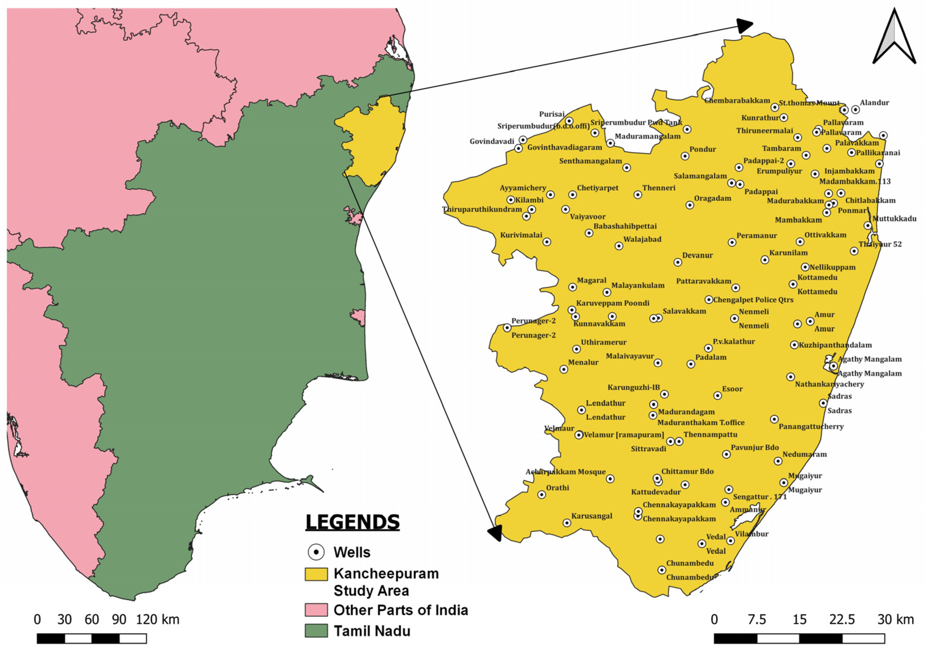
3.1. Study Area

The study area selected for this research is the Kanchipuram district, Tamil Nadu, India. Figure 1 shows the study area, one of the thirty-eight districts (in the northeast) of Tamil Nadu in India. Villupuram District in the south, Thiruvallur and Chennai districts in the north, Tiruvannamalai and Vellore districts in the west, and the Bay of Bengal in the east define Kanchipuram District. This district is located between 12°14′00″ N and 13°02′00″ N latitude and 79°31′30″ E and 80°15′30″ E longitude, with a total area of 4307 sq. km². The district is divided into 13 blocks, 633 villages, and 4015 habitations. The type of soil in Uthiramerur blocks of the district is red loam and lateritic soil in plateau areas, black soil is spread in all blocks of the district, and a sandy coastal alluvial type is found in Thirukazhukundram, Thiruporur, and St. Thomas Mount.

Sedimentary and fractured rocks coexist in the area. Weathered, unconsolidated, and semi-consolidated formations and fissured and fractured crystalline rocks comprise the important aquifer system in the Kanchipuram district. Researchers analyzed data from 129 monitoring wells installed by the Tamil Nadu Water Supply and Drainage Board (TWAD) from March through May, October, and November to determine seasonal changes in groundwater quality and levels. The water used by the Chennai Metropolitan Area comes from several storage tanks and groundwater wells in this study area.

3.2. Water Quality in the Study Area

Rainfall is the primary source of both surface and subsurface water availability. Based on the monsoon, the intensity of rainfall changes from year to year, and rainfall data for the Kanchipuram district may be seen in

Table 1. Rainfall data in Kanchipuram District.

Annual Rainfall (mm)								Average Annual Rainfall (mm)
2013	2014	2015	2016	2017	2018	2019	2020
905.2	907.9	2256.6	990.5	1191.7	712.73	1215.5	985.36	1252

. Chembarambakkam Lake and Madurantakam Lake are important lakes in the Kanchipuram district, supplying drinking water to the city of Chennai. The extraction of surface and subsurface water, on the other hand, is increasing yearly. It has an environmental impact on water supplies, such as water level depletion and water quality degradation. It creates a demand for the quantification of accessible water and its quality for various reasons, including agriculture, industry, drinking water, and domestic use.

The only exception is in and around the Kazhuveli tank, where the water could be better due to seawater intrusion in the lagoons during high tide seasons, salt manufacture, and aquaculture cultivation. Groundwater quality in Kanchipuram District ranges from moderate (palatable water) to good (potable water) in both shallows dug wells and bore wells.

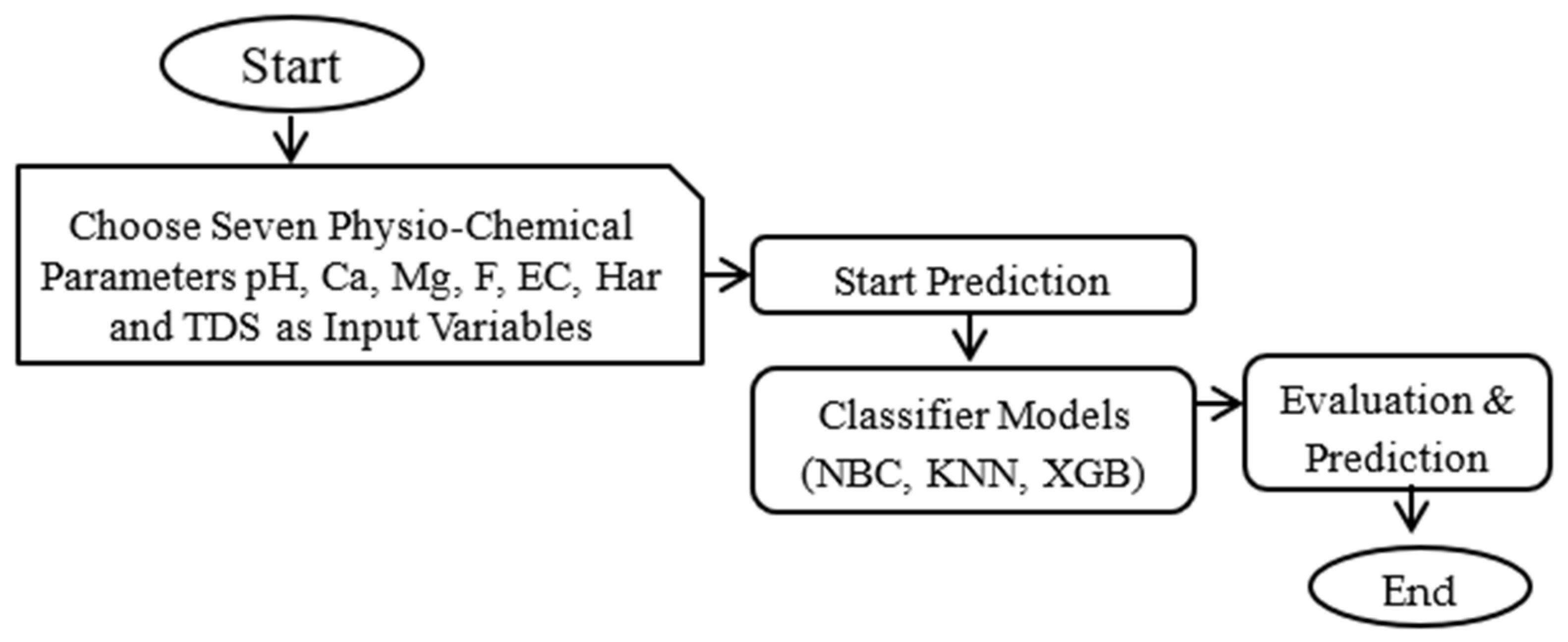
3.3. Research Methodology

Figure 2 depicts the proposed study design technique for the water quality prediction system. Data pre-processing is the first step, including data cleaning and feature selection. The process of deleting missing or unsuitable (incomplete or duplicate) records from a dataset is known as data cleaning. Choosing the most significant feature that increases the prediction variable’s value is known as feature selection. Groundwater assessment is conducted for the wells by the Pollution Control Board (PCB), Government of Tamil Nadu, to assess pumping level and water quality. Many other parameters include TDS, SO₂, NO₂, CA, MG, Na, K, Cl, SO₄ CO₃, HCO₃, F, etc. In this work, seven parameters, pH, calcium (Ca), magnesium (Mg), fluoride (F), hardness (Har), total dissolved solids (TDS), and electrical conductivity (EC), are selected for model development. Thus, the model gives the best accuracy. After computing the GQI, we can sort the information into appropriate categories and use the World Health Organization’s guidelines to determine whether or not a certain water supply is safe for human consumption. So, we have binary (healthy and unhealthy water samples) and multiclass (poor, bad, average, good, and excellent water samples) representations of the data. Once the input dataset is fully classified, we split it into training and testing sets.

Only 30% of the data are used for testing, whereas 70% are used for training. Classifier models utilized during training include the naïve Bayes classifier, the KNN classifier, and the XGBoost classifier. The assessment of the models’ precision and accuracy is carried out. Each of these classifiers brings unique strengths to the task of predicting the GQI. Bayesian classifiers are known for their simplicity and can perform well when data exhibit clear class separability. KNN classifiers are effective when dealing with spatial or temporal patterns often present in water quality data. XGBoost, as an ensemble method, can capture complex relationships between variables and has been successful in various predictive modeling tasks. In addition, an LSTM-based model for water quality predictions over the next five years is created. The choice of machine learning models, like LSTM, XGBoost, KNN, and naïve Bayes, over others in this research paper can be attributed to their suitability for the specific research tasks, their previous success in similar domains, their benchmark status, and considerations related to complexity, interpretability, computational resources, expertise, data characteristics, and research focus. We compare results from various machine learning models to identify the one best suited for our application. The best possible model is then used to predict the water’s quality.

3.4. Collection and Pre-Processing of Data Analysis

To make predictions in data processing, we employ four suitable measures of data collection, description, partitioning, and the use of the water quality index (WQI). We can evaluate water quality in four different ways. Data are currently being generated at an unprecedented rate in various formats, including numeric, categorical, and free-text data. Acquiring and analyzing data from diverse sources is achieved through data collection. For data to be used in creating effective AI and machine learning solutions, they must be collected and organized in a way that aligns with the specific situation. Analyzing collected data for recurring patterns enables us to monitor past events. Machine learning algorithms actively seek out patterns and extrapolate their implications for the future, aiding in the construction of predictive models. Precise predictions rely on the quality of data used to build predictive models, emphasizing the importance of efficient data gathering methods that provide reliable and relevant information for the intended purpose. This study utilized data from wells in the Kanchipuram district. The dataset comprises monthly water statistics collected for five years (2015–2019) before and after the monsoon season, encompassing seven crucial factors, TDS, Ca²⁺ Mg²⁺, Fl, EC, total hardness, and pH, extracted from a dataset of 1171 records. Figure 3 illustrates the locations of the 129 wells in the Kanchipuram district from which data were collected for this research. The focus was placed on specific parameters: pH, electrical conductivity, total dissolved solids, and total hardness, as they are commonly measured and carry significant implications for groundwater quality. The exclusion of other parameters such as phosphate (PO₄), nitrate, biochemical oxygen demand (BOD), chemical oxygen demand (COD), dissolved oxygen (DO), and temperature was due to factors like data availability, specific research goals, and the feasibility of including numerous parameters in the GQI calculation. As

Table 2. Quality Standards for Drinking Water.

Parameters	WHO		Indian Standards [36]
	Desirable	Excessive	Desirable	Excessive
pH (no unit)	7–8.5	6.5–9.2	6.5–8.5	6.5–9.2
Turbidity (NTU)	5	50	10	25
Total Solids (mg/L)	500	1500	---	---
Total Hardness (mg/L)	250		300	600
Calcium (mg/L)	75	200	75	200
Magnesium (mg/L)	50	150	30	100
Iron (mg/L)	0.3	1	0.3	1
Chlorides (mg/L)	200	600	250	1000
Alkalinity (mg/L)	---	---	200	600
Dissolved Solids (mg/L)	---	---	500	2000

indicates, multiple criteria are available to assess the suitability of a given groundwater sample for use.

Figure 4 and Figure 5 show the TDS and Ca changes from 2015 to 2019 in the study area. It is observed that these two water quality parameters change from location to location over time. The TDS value is excessive according to the standards presented in Table 2. Similarly, the changes observed for calcium are illustrated in Figure 5, which indicates that the calcium level is more than 200 mg/L in a particular area due to groundwater contamination.

The dataset, in the context of machine learning and deep learning, is a set of 1171 real-world data entries, each characterized by seven parameters related to drinking water quality. These parameters are compared against an ideal range (as shown in Table 2) to assess water quality. Data splitting is a critical process in the machine learning workflow, primarily used for cross-validation. It involves dividing the available data into two distinct subsets:

Training Set: This portion of the dataset, which consists of 819 samples (approximately 70% of the total data), is used to build and train the predictive model. During training, the model learns the underlying patterns and relationships within the data.

Testing Set: The remaining portion of the dataset, comprising 352 samples (about 30% of the total data), serves as an independent evaluation set to assess the effectiveness and generalization of the trained model. It simulates the model’s performance on new, unseen data.

The main challenge faced by machine learning and deep learning practitioners during data splitting is achieving an appropriate balance between the sizes of the training and testing sets. There need to be more data for training and testing to avoid unpredictable model results, potentially resulting in overfitting (where the model fits the training data too closely and performs poorly on new data) or underfitting (where the model is too simplistic and fails to capture underlying patterns).

To address these concerns and guarantee dependable model performance, it is imperative to meticulously divide the data into training and testing datasets. In this instance, a partitioning ratio of 70:30 was employed, leading to 819 samples for training and 352 samples designated for testing. This process allows for thorough model evaluation and ensures that the model can make accurate predictions on unseen data, ultimately contributing to the accuracy and reliability of inferences made by the machine learning model.

It is essential that some water quality parameters, such as pH, electrical conductivity, total dissolved solids, and total hardness, are typically included in the calculation of a groundwater quality index (GQI); other environmental factors like rainfall and groundwater levels may not be direct components of the GQI itself. However, these factors can indirectly impact groundwater quality and may be considered part of a broader assessment of groundwater conditions. Figure 6 shows the observed TDS values from 2015 to 2019 in the study area using QGIS version 3.22 open-source software. The collected data were used to develop this map. Due to the urban expansion of Chennai, the Alandur and Tambaram taluks exhibit very low quality. Due to the increased industrial concentration, high population density, and urbanization in Sriperumbathur, the region’s groundwater quality could improve during the pre-monsoon season. Figure 7 illustrates the critical water quality parameters observed for 2019 in the GIS.

3.5. Description and Splitting of Dataset

The dataset contains 1171 entries in a multiclass classification with seven parameters. Table 2 shows the ideal range of parameters for drinking water. The act of partitioning available data into two sets, common for cross-validation purposes, is known as data splitting. One part of the data is used to create a predictive model, while the other assesses the model’s effectiveness. The most difficult challenge faced by ML/DL practitioners is dividing data for training and testing. Unpredictable results from the model can be the result of insufficient training and testing data. It may lead to either overfitting or underfitting the data, producing inaccurate inferences. The data must be split into training and testing sets before the machine learning model can be trained. Once the data have been partitioned, the model is trained and evaluated on subsets of the data to determine its efficacy. For both training and testing purposes, data were split into 30:70 percentiles. In total, 1171 samples were used; 819 for training and 352 for testing. Instead of having a dedicated validation set, it is chosen to use techniques like K-fold cross-validation on the training set to estimate model performance. Cross-validation involves splitting the training data into multiple subsets, training the model on different combinations, and using these subsets for validation iteratively. This approach allows for a more robust assessment of model performance while making efficient use of the available data.

3.6. The Proposed ML Model

The samples collected contain the chemical composition and statistical information of water from wells, as mentioned in Figure 3, in the Kanchipuram district. The water samples have to be identified for fitness for drinking based on the various available parameters such as total dissolved solids (TDS), magnesium (Mg²⁺), calcium (Ca²⁺), sodium (Na⁺), fluoride (F⁻), potassium (K⁺), nitrates (NO₂⁺NO₃), chlorine (Cl⁻), sulfate (SO₄²⁻), carbonate (CO₃²⁻, HCO³⁻), pH level, electrical conductivity (EC), and total hardness (TH). The major parameters we considered in this work are pH, Ca, Mg, Fl, EC, HAR, and TDS, which greatly impact the water quality. Machine learning models create predictions based on previously collected data. The overall architecture of the proposed work is shown in Figure 8.

3.6.1. Naïve Bayes Classifier

We can utilize machine learning to develop models for classifying items based on their characteristics. Researchers applied the Bayes theorem to establish a category of classification algorithms, famously recognized as naïve Bayes classifiers. This category of algorithms guarantees that no two pairs of classified qualities depend on each other. A naïve Bayes classifier, a probabilistic machine learning model, is used to complete classification tasks. The Bayes theorem is the foundation of the classifier. Bayes’ theorem can be used to determine the probability of event A given event B. The data support hypothesis B, while A is speculative. In this scenario, the predictors/features are unrelated to one another. In other words, the presence of one quality has no bearing on the other, making it naïve. They are quick and simple to implement, but their major drawback is the predictors’ necessity to be independent.

The predictors usually depend on real-life situations, limiting the classifier’s effectiveness. The Bayesian technique uses statistics and blends prior and posterior probability to reduce bias and overfitting. The naïve Bayes method is a classification model based on Bayes’ theorem that is unaffected by characteristic conditions. When the target value is known, the technique used in the Bayesian approach, such as uncorrelated attributes, makes the procedure relatively straightforward to apply to the features. The independence in attributes, represented by Bayes theorem in Equation (1), is used in the naïve Bayes classifier.

$$\mathrm{P}(\mathrm{a}|\mathrm{b})={\displaystyle \frac{P\left(b|a\right)P\left(a\right)}{P\left(b\right)}}$$

(1)

The likelihood of a prediction given a class, denoted by P(b|a), and the prior probability of a prediction, denoted by P(b), yield the posterior probability of class, denoted by P(a|b). A prior probability of 0.5 is tried for naïve Bayes.

3.6.2. KNN Classifier

Since the early 1970s, researchers have employed KNN as a non-parametric method for statistical estimation and pattern identification. In this approach, a case is assigned to the class encompassing most of its K-nearest neighbors, determined using a specific distance function. The example belongs to the category of the person to the left of it if K = 1. The K-nearest neighbors (KNN) algorithm is an easy-to-implement supervised machine learning technique that may be used to solve classification and regression problems. KNN suggests placing comparable items nearby.

Items of a similar nature are situated near one another. The best way to find the right value for K is to look at the data first. In most cases, the higher the K, the more precise the result will be because it will have less total noise. Another technique for obtaining a suitable K value in hindsight is cross-validation, which involves verifying the K value with a different dataset. Historically, the optimal K for most datasets has been around 3 to 10.

KNN’s main drawback is that it becomes increasingly slow with increasing input volume, making it inappropriate when fast predictions are needed. The classification and regression outcomes offered by faster algorithms can also be more reliable. Conversely, if enough computational resources are available to manage the data required to create predictions fast, KNN might be useful in tackling issues whose solutions rely on finding related things. The KNN classifier makes its determinations by comparing associated features. Each data point is assigned a label depending on the labels of its neighbors. KNN catalogs all available samples and sorts them according to some similarity measure. K in KNN is the number of nearest neighbors used in the majority voting. Parameter tuning entails settling on an optimal value for K to maximize precision. To avoid mixing up two datasets (specifically, when n represents the total number of observations and K is an odd value, such as sqrt(n)), practitioners employ KNN. KNN is applied when the dataset is small, the data contain labels, or the data are clean and sometimes even in cases where all these conditions are met. The design parameters tried with KNN are 5 neighbors, Euclidean distance, and the kd-tree algorithm. To obtain the Euclidean distance between two points on a plane identified by their coordinates (x, y) and (a, b), one uses the following formula:

$$\mathrm{Dist}(\mathrm{d})=\sqrt{{(x-a)}^2+{(y-b)}^2}$$

(2)

3.6.3. XGBoost Classifier

In ensemble learning, boosting combines weak classifiers to create robust ones, addressing the bias–variance trade-off. Boosting techniques are vital for managing both bias and variance, in contrast to bagging algorithms, which primarily focus on reducing variance within a model. The acronym “XGBoost” stands for “extreme gradient boosting”. XGBoost is an optimized, flexible, and portable distributed gradient boosting toolbox that employs a method known as parallel tree boosting to efficiently tackle various data science problems. A regularization term is used to smooth out the final learning weights, reducing overfitting and favoring models with simpler prediction functions. For tree ensemble models, traditional optimization methods in Euclidean space are ineffective. Instead, an additive approach is used for model training. Additionally, two protective measures are employed to prevent overfitting. The initial strategy of shrinkage, proposed by Friedman, involves adjusting the newly added weights by a factor after each iteration of tree boosting.

Shrinkage, which can be likened to a learning rate in stochastic optimization, diminishes the importance of each tree, enabling the model to accommodate additional trees added later. The second method, subsampling by column (feature), is employed by random forest. Avoiding overfitting is generally more manageable with row subsampling compared to column subsampling. Using column subsamples enhances the speed of calculations in the parallel algorithm. The XGBoost algorithm is an ensemble technique that combines multiple models to create the final model, resulting in effective outcomes through an incremental approach. Instead of training a single model with all potential parameters, each subsequent model is trained to rectify the errors of the preceding one. Models are added one by one until further improvement becomes unattainable. The approach adopted in XGBoost is illustrated in Figure 9.

A robust neural network capable of handling sequence dependencies is the recurrent neural network (RNN). The LSTM network, a specific type of RNN, is employed to predict time series sequences. This network addresses the issue of vanishing gradients through back propagation, making LSTM the most suitable network for predicting time series sequences. LSTM is conceptualized as a sequence of blocks for learning time series sequences. It features three critical gates: the forget gate, the input gate, and the output gate. These gates manage the addition or removal of data from the current cell state, represented by a line from Ct-1 to Ct, as depicted in Figure 10.

XB_par = {‘max_depth’:[2, 3, 5], ‘learning_rate’:[0.01, 0.1, 0.5, 1], ‘n_estimators’:[50, 100, 150, 200, 300], ‘gamma’:[0, 0.001, 0.01, 0.1]}

3.6.4. LSTM Network

Forget gate: This gate examines the values h_t−1, previously hidden layer output, and x_t, the current input, and returns a value between 0 and 1 for the input available during previous cell state C_t−1, with 1 representing retaining the value in the previous state C_t−1 and 0 representing discarding it.

$$f_t=\sigma (W_f·\left[C_{t-1},h_{t-1},x_t\right]+b_f)$$

(3)

In Equation (3) above, the forget gate’s output is represented by the sigmoid function ft. Both the forget gate’s weight (Wf) and bias (bf) are optional.

Input gate: This layer determines what fresh data should be added to the current state of the cell. The sigmoid layer of the input gate first filters information from ht−1, xt, and Ct−1, as shown in Equation (4), and then the tanh layer builds a vector consisting of all potential values added to the cell state with a value between −1 and 1. This is the result of the input gate’s logic operation. In the formula, Wi and bi represent the weight and bias of the input gate. Weight (Wc) and bias (bc) stand for the cell state in Equation (5).

$$i_t=\sigma (W_i·\left[C_{t-1},h_{t-1},x_t\right]+b_i)$$

(4)

$$C_t=tanh(W_c·\left[h_{t-1},x_t\right]+b_C)$$

(5)

Output gate: This gate determines the cell state value to be output. To begin sending only some aspects of the cell’s condition, a sigmoid layer needs be developed. After the tanh layer performs an adjustment between −1 and 1, the sigmoid layer’s output is multiplied by the cell state value. Ot represents the output of the output gate, Wo and bo represent the weight and bias supplied by the input gate to the output gate, and ht represents the current output of the hidden layer in Equations (6) and (7).

$$O_t=\sigma (W_o·\left[C_t,h_{t-1},x_t\right]+b_o)$$

(6)

h_t = O_t ∗ tanh (C_t)

(7)

Using Keras, we construct a sequential model to add layers sequentially. The first layer is designed with 50 LSTM units. Following the LSTM layer, we apply a dropout layer with a dropout rate of 0.2 to mitigate overfitting. We employ the mean squared error as the loss function to assess the model’s performance. The model calculates the loss for each epoch and updates the weights accordingly. A lag time of 6 months is selected in this work. The best combination of the given parameters is selected for water quality prediction.

4. Results and Discussion

4.1. ML-Based Prediction Results

The pH, calcium, magnesium, fluoride, total hardness, total dissolved solids, and electrical conductivity of water samples collected in the Kanchipuram district are measured. The WQI was computed using the weighted arithmetic method, as shown in Equation (8).

$$\mathrm{WQI}={\displaystyle \frac{\sum _{i=1}^n{w}_i{q}_i}{\sum _{i=1}^n{w}_i}}$$

(8)

where n is the total number of attributes, wi is weight, and qi is quality in terms of water. The following Equation (9) to determine the value of qi:

q_i = 100[(V_i − V_id)/(S_i − V_id)]

(9)

where Vi is the measured value, Si is the recommended maximum, and Vid is the ideal value found in pure water. All ideal values (Vid) for potable water are zero [37], with the exception of pH and DO. While a pH of 7.0 is considered optimum for pure water, a value of 8.5 is considered acceptable for water that has been exposed to pollution. Therefore, the following Equation (10) is used to determine the pH quality grade.

q_pH = 100[(V_pH − 7.0)/(8.5 − 7.0)]

(10)

According to Brown et al., [38],

Table 3. Weighted arithmetic method for Water quality classification.

GQI	Status
0–25	Excellent
26–50	Good
51–75	Poor
76–100	Very poor
Above 100	Unsuitable for drinking

illustrates a categorization of water quality. This classification is based on the observed value of dissolved oxygen, which is denoted by VpH.

Table 4. Computation of the WQI for Kanchipuram District.

Parameter	Observed Values (vi)	Standard Values (Si)	Unit Weights (wt)	Quality Rating (qi)	Wiqi
pH	8.4	6.5–8.5	0.116909012	93.33332	10.91150667
Ca	114 mg/L	75 mg/L	0.013249688	152	2.0139526
Mg	15.795 mg/L	30 mg/L	0.03312422	52.65	1.743990183
F	0.1 mg/L	1.2 mg/L	0.828105503	8.333333	6.900879192
EC	1610 mg/L	300 mg/L	0.003312422	536.6667	1.777666473
Har	350 mg/L	300 mg/L	0.003312422	116.6667	0.38644923
TDS	947 mg/L	500 mg/L	0.001987453	189.4	0.376423598

lists the observed values (vi) for the seven physicochemical parameters of the water sample from Well 13206, the drinking water values (Si), the unit weights (wi), the water quality rating (q_i), and the w_iq_i.

The GQI at a specific well in the Kanchipuram district is then calculated using an arithmetic mean and applied to the water status specified in Table 3. As a result, this water quality study of various wells in the Kanchipuram district aids in determining the water’s acceptability for consumption. A machine learning algorithm makes it simple to assess water quality before it is planned for public use. The experimental results show that the prediction of water quality obtained using the above-proposed methods is close to the actual result. The distribution of five different classes of training samples, excellent, good, poor, very poor, and unfit for drinking, is shown in Figure 11. The confusion matrix for naïve Bayes, KNN, and XGBoost classifiers is presented in

Table 5. Confusion Matrix for Various Classifiers.

Classifier	Rating	Excellent	Good	Poor	Unfit	Very Poor
Naïve Bayes classifier	Excellent	54	11	0	0	0
	Good	3	161	3	0	0
	Poor	0	18	57	0	4
	Unfit	0	0	0	10	7
	Very Poor	0	0	1	0	23
KNN classifier	Excellent	64	1	0	0	0
	Good	5	158	4	0	0
	Poor	0	7	72	0	0
	Unfit	0	0	0	16	1
	Very Poor	0	0	5	1	18
XGBoost classifier	Excellent	63	2	0	0	0
	Good	1	163	3	0	0
	Poor	0	7	72	0	0
	Unfit	0	0	0	16	1
	Very Poor	0	0	4	1	19

.

Naïve Bayes, KNN, and XGBoost are trained with the dataset with five different categories. The model is assessed using the resulting confusion matrix with the remaining test set for accurate prediction. The confusion matrices of various classifiers are compared and analyzed for better performance. The confusion matrix shows the link between the actual and intended classes.

The analysis of confusion matrices of different classifiers shows that water with excellent and good quality is never classified as unfit for drinking or very poor. Similarly, water in unacceptable and very poor classes is never classified as excellent or good. Thus, misclassification occurs among closer classes such as excellent and good. As a result, using these machine learning techniques to determine water quality is highly recommended. Still, the performance of the algorithms can be fine-tuned to come closer to the original results. The percentage of samples accurately predicted is known as accuracy. It is the most significant indicator for assessing the model’s performance. Accuracy is calculated by dividing the number of right guesses by the total number of forecasts as below:

(TN + TP)/(TN + TP + FN + FP)

where TN denotes true negative, which indicates water that is unfit for drinking as unacceptable correctly. FP denotes false positive, which shows that poor-quality water is excellent. TP denotes true positive, which accurately indicates good-quality water as good. FN denotes false negative, which means excellent water is classified as unfit for drinking.

In this work, seven parameters, pH, calcium (Ca), magnesium (Mg), fluoride (F), hardness (Har), total dissolved solids (TDS), and electrical conductivity (EC), are selected. PCA can also be applied to reduce the number of features as suggested.

Figure 12 shows the ROC curves plotted for the XGBoost classifier. The ROC curve obtained for the classifier lies farther from the diagonal line, and AUC values are equal to 1. Thus, the model gives the best accuracy. It is possible to address the issues related to uncertainty, reliability, and resiliency of the MLMs by comparing the performance of the models with real-time data input.

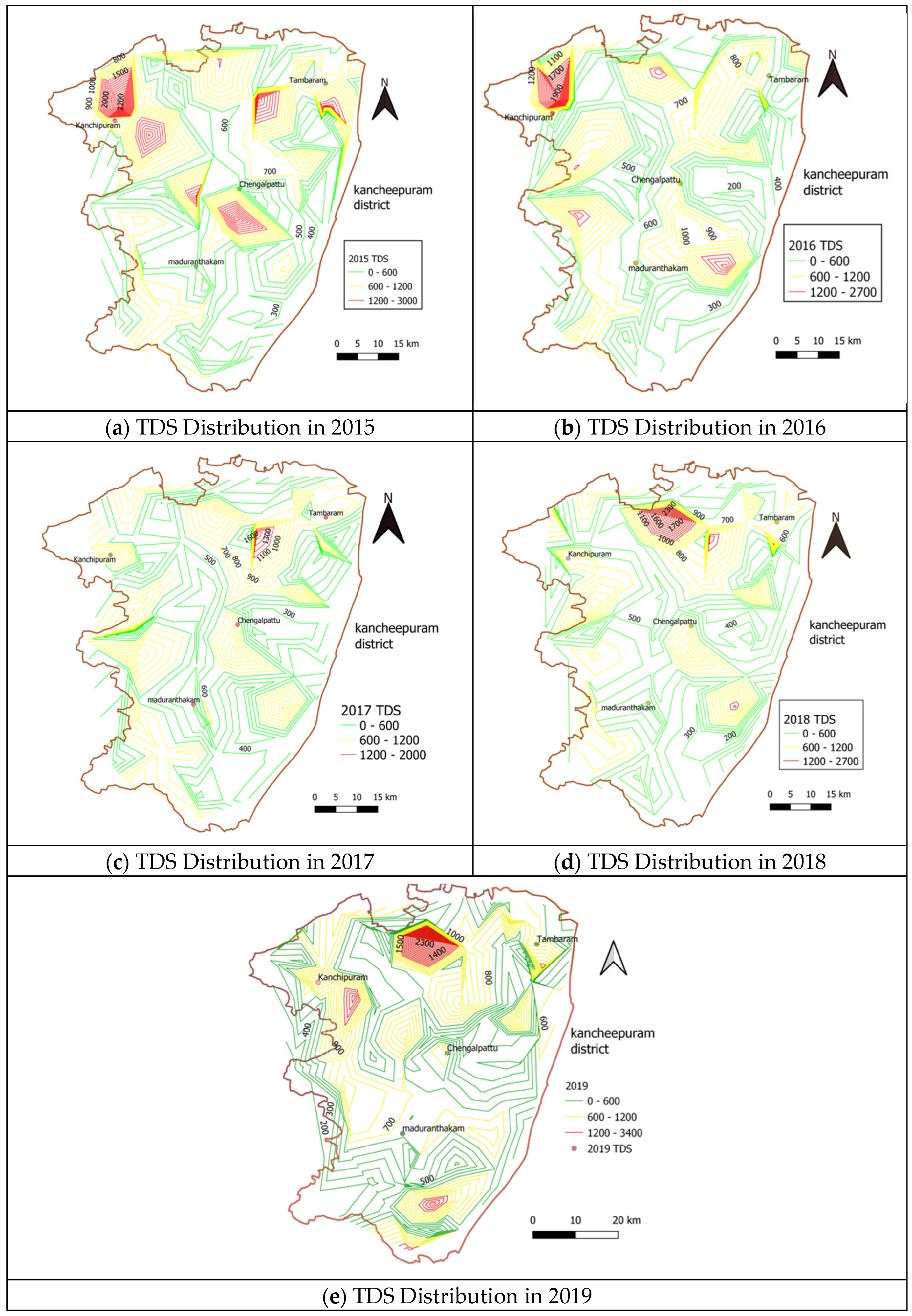
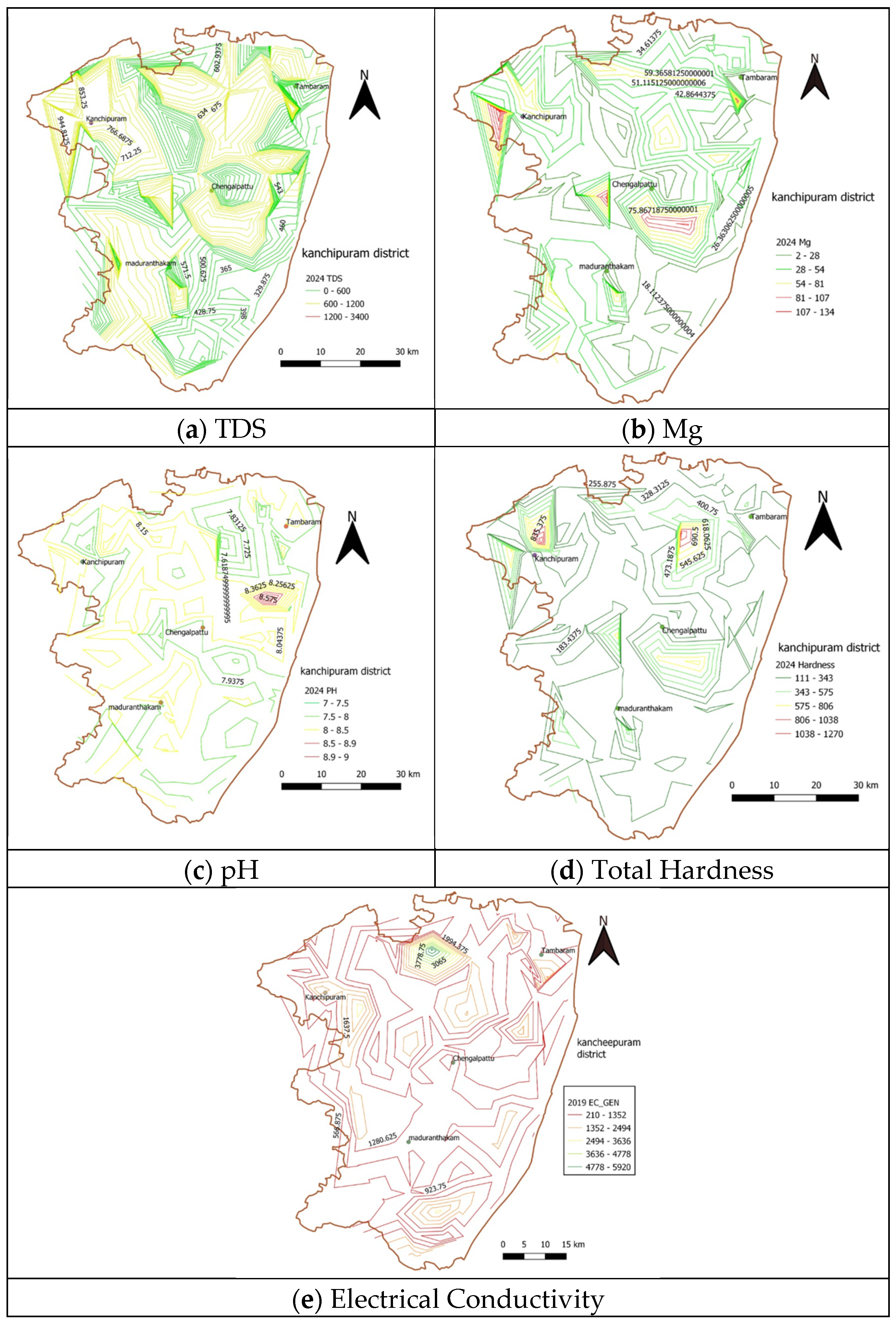
4.2. GIS-Based Water Quality Analysis

In order to present and observe the LSTM models’ anticipated values in the areas where the quality will be undesirable in the future, they are exported to a GIS environment, as shown in Figure 13.

Figure 13 a–e shows that the water quality in the study region is degrading due to the activities in the surrounding neighborhoods. As shown in Figure 13a, the TDS value has significantly fluctuated in the research area. Figure 14a shows the graph for pH values observed and predicted from 2014 to 2024 in two colors. This plot shows that in the marked period till 2019, the pH value changed between 7.6 and 8.3, but in the predicted period from 2020 to 2024, the pH value is from 7.35 to 8.

Due to the machine learning model application, the prediction values are good. Figure 14b shows the plot between the observed TDS and predicted values from 2014 to 2024. The machine learning model performs extremely well in TDS prediction, as shown in Figure 14b. The calculated GQI and predicted GQI are presented in Figure 14c for the study area. The calculated values of the GQI change according to the plot’s groundwater quality and rainfall data. However, the predicted values of the GQI change based on the seasonal variations of the groundwater parameters, resulting from the rainwater and nature of activities in the study area. It is further seen from Figure 14c during the summer seasons that the water quality is higher and lower during winter. Hence, rainwater is the main source for the GQI in the study area, which helps in the extraction of water plans for the urban planners in the study area. The prediction of the GQI for the next five years based on five years of known data is reasonable since it depends on the stability of water quality parameters, temporal trends, data representativeness, rigorous model validation, and continuous monitoring and adaptation to changing conditions.

Further, the prediction interval can be varied according to the user’s requirement. The LSTM model is evaluated based on root mean squared error. The very low value of RMSE (0.014) justifies the reliable prediction. The accuracy calculated for the various applied machine learning algorithms is important for analyzing the research output. The performance comparison of all the algorithms is shown in Figure 15. The comparison indicates that XGBoost outperforms the other classifiers, KNN and naïve Bayes. The water quality prediction model may thus replace the water quality testing process at laboratories involving many hours of laborious work.

Table 6. Comparison between different Water Quality prediction models.

Prediction Model Proposed by	ML Technique Used	Location	Data Collection Duration	Time Horizon	Performance Metrics
[39]	Support vector regression	Jialing River, China	One year	Weekly	MAE: 0.175 MAPE: 2.153% RMSE: 0.228 R2: 0.919
[40]	Random forest classifier	-	-	-	Accuracy: 100% F1 score: 1.0
[41]	M5 model	Hamedan (Iran)	Ten years	-	RMSE values is reduced by 18.95%
[42]	Stacking ensemble	-	-	-	Highest performance among all the other individual classifiers
[43]	Support vector regression	China	Four years	-	RMSE: 0.251, MSE: 0.063, MAE: 0.190, R2: 0.911
[44]	ANFIS-PSO	Allen County, Indiana	-	-	RMSE: 1.284
Proposed model	XGBoost KNN Naïve Bayes	Chennai, India	Five years	6 months	Accuracy: 94.6% RMSE: 0.014

provides an overview of various models developed by researchers and applied worldwide. It can be seen that the model proposed in this research yields better results than those of other researchers.

5. Conclusions

The ability to model and forecast water quality is critical for environmental protection. Machine learning algorithms have recently found use in practically every industry and have thus been used to develop a water quality forecast model that is close to reality. This research uses machine learning classifier approaches such as naïve Bayes, KNN, and XGBoost and applies LSTM to build water quality prediction models. The confusion matrices and accuracy are used as the statistical parameters to evaluate and analyze the developed models. Based on the obtained results, XGBoost outperforms the other two algorithms in predicting water quality with an accuracy of 94.6%. Careful analysis reveals that the proposed conceptual methods can soon forecast water quality in the Kanchipuram district. Statistical analysis was used to summarize and evaluate the proposed methodology. Using GIS and soft computing tools to monitor the GQI, the following conclusions can be drawn:

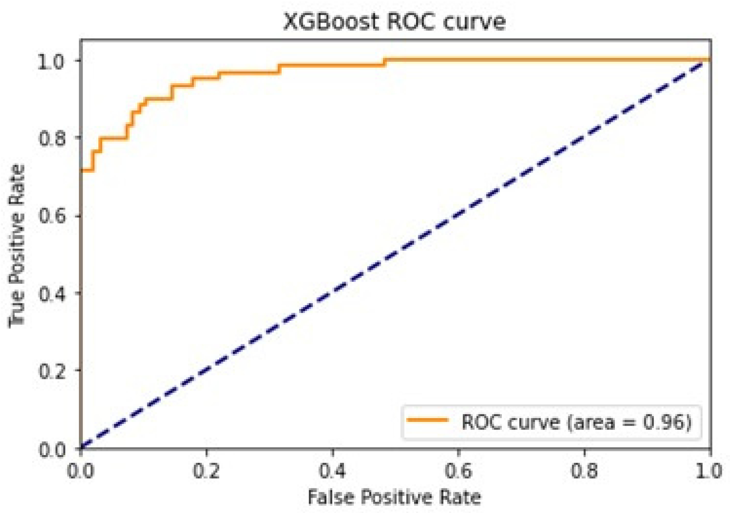
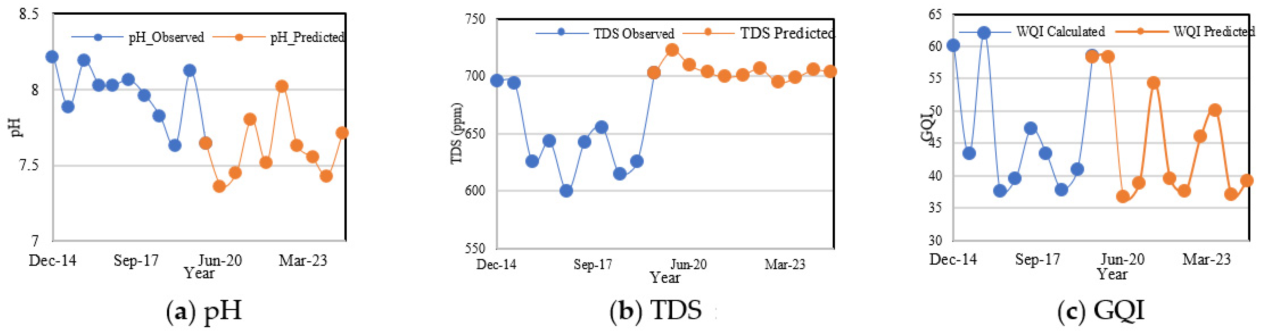
• First, machine learning algorithms, namely, naïve Bayes, KNN, and XGBoost, can be developed for the GQI. XGBoost outperforms KNN and naïve Bayes in the WQI. The results reveal that the XGBoost classifier model yielded the highest accuracy of about 94.6%, which surpassed the existing results. The predicted results using LSTM for the next five years indicate a reliable approach for forecasting the water quality.
• Thus, the proposed hybrid prediction model will identify any degradation in water quality before being planned for human consumption and can be used to notify the appropriate authorities. This research identifies the locations/places where water quality control measures or management measures are required in 2024.
• In the pre-monsoon season, the GQI is found to be poor in taluks such as Alandur, Tambaram, and Sriperumpudur. Compared to other taluks, these areas have the highest population density and urbanized areas. Cheyyur, Tirukalukundram, Chengalpattu, and Madurandagam taluks have excellent groundwater quality in the pre-monsoon season.

References

1. Aendo, P.; Netvichian, R.; Thiendedsakul, P.; Khaodhiar, S.; Tulayakul, P. Carcinogenic Risk of Pb, Cd, Ni, and Cr and Critical Ecological Risk of Cd and Cu in Soil and Groundwater around the Municipal Solid Waste Open Dump in Central Thailand. J. Environ. Public Health. 2022, 2022, 3062215. [Google Scholar] [CrossRef] [PubMed]
2. Chapman, D.V.; World Health Organization; UNESCO & United Nations Environment Programme. Water Quality Assessments: A Guide to the Use of Biota, Sediments and Water in Environmental Monitoring; Chapman & Hall: London, UK, 1992. [Google Scholar]
3. Li, W.; Chai, Y.; Khan, F.; Jan, S.R.U.; Verma, S.; Menon, V.G.; Kavita; Li, X. A Comprehensive Survey on Machine Learning-Based Big Data Analytics for IoT-Enabled Smart Healthcare System. Mob. Networks Appl. 2021, 26, 234–252. [Google Scholar] [CrossRef]
4. Jha, M.K.; Shekhar, A.; Jenifer, M.A. Assessing groundwater quality for drinking water supply using hybrid fuzzy-GIS-based water quality index. Water Res. 2020, 179, 115867. [Google Scholar] [CrossRef] [PubMed]
5. Chen, K.; Chen, H.; Zhou, C.; Huang, Y.; Qi, X.; Shen, R.; Liu, F.; Zuo, M.; Zou, X.; Wang, J.; et al. Comparative analysis of surface water quality prediction performance and identification of key water parameters using different machine learning models based on big data. Water Res. 2020, 171, 115454. [Google Scholar] [CrossRef] [PubMed]
6. Shams, M.Y.; Elshewey, A.M.; El-kenawy, E.-S.M.; Ibrahim, A.; Talaat, F.M.; Tarek, Z. Water quality prediction using machine learning models based on grid search method. Multimed. Tools Appl. 2023, 83, 35307–35334. [Google Scholar] [CrossRef]
7. Cheng, B.; Zhang, Y.; Xia, R.; Wang, L.; Zhang, N.; Zhang, X. Spatiotemporal analysis and prediction of water quality in the Han River by an integrated nonparametric diagnosis approach. J. Clean. Prod. 2021, 328, 129583. [Google Scholar] [CrossRef]
8. Al-Adhaileh, M.H.; Alsaade, F.W. Modelling and prediction of water quality by using artificial intelligence. Sustainability 2021, 13, 4259. [Google Scholar] [CrossRef]
9. Hejaz, B.; Al-khatib, I.A.; Mahmoud, N. Domestic Groundwater Quality in the Northern Governorates of the West Bank, Palestine. J. Environ. Public Health. 2020, 2020, 6894805. [Google Scholar] [CrossRef]
10. Oberascher, M.; Rauch, W.; Sitzenfrei, R. Towards a smart water city: A comprehensive review of applications, data requirements, and communication technologies for integrated management. Sustain. Cities Soc. 2022, 76, 103442. [Google Scholar] [CrossRef]
11. DeSimone, L.A.; Pope, J.P.; Ransom, K.M. Machine-learning models to map pH and redox conditions in groundwater in a layered aquifer system, Northern Atlantic Coastal Plain, eastern USA. J. Hydrol. Reg. Stud. 2020, 30, 100697. [Google Scholar] [CrossRef]
12. Elubid, B.A.; Huang, T.; Ahmed, E.H.; Zhao, J.; Elhag, K.M.; Abbass, W.; Babiker, M.M. Geospatial Distributions of Groundwater Quality in Gedaref State Using Geographic Information System (GIS) and Drinking Water Quality Index (DWQI). Int. J. Environ. Res. Public Health. 2019, 16, 731. [Google Scholar] [CrossRef] [PubMed]
13. Matsui, K.; Kageyama, Y. Water pollution evaluation through fuzzy c-means clustering and neural networks using ALOS AVNIR-2 data and water depth of Lake Hosenko, Japan. Ecol. Inform. 2022, 70, 101761. [Google Scholar] [CrossRef]
14. Watershed, E.L.; Wang, X.; Zhang, F.; Ding, J. Evaluation of water quality based on a machine learning algorithm and water quality index for the. Sci. Rep. 2017, 7, 12858. [Google Scholar] [CrossRef]
15. Malakar, P.; Mukherjee, A.; Bhanja, S.; Saha, D.; Ray, R.K.; Sarkar, S.; Zahid, A. Importance of spatial and depth-dependent drivers in groundwater level modeling through machine learning. Hydrol. Earth Syst. Sci. Discuss. 2020, 2020, 1–22. [Google Scholar] [CrossRef]
16. Uddin, G.; Nash, S.; Olbert, A.I. A review of water quality index models and their use for assessing surface water quality. Ecol. Indic. 2021, 122, 107218. [Google Scholar] [CrossRef]
17. Mallick, J.; Talukdar, S.; Pal, S.; Rahman, A. A novel classifier for improving wetland mapping by integrating image fusion techniques and ensemble machine learning classifiers. Ecol. Inform. 2021, 65, 101426. [Google Scholar] [CrossRef]
18. Perez, J.; Attanasio, A.C.; Nechyporenko, N.; Sanz, P.J. A Deep Learning Approach for Underwater Image Enhancement. In Biomedical Applications Based on Natural and Artificial Computing: International Work-Conference on the Interplay Between Natural and Artificial Computation, IWINAC 2017, Corunna, Spain, 19–23 June 2017; Springer International Publishing: Berlin/Heidelberg, Germany, 2017; pp. 183–192. [Google Scholar] [CrossRef]
19. Babak, S.; Seyed, H.; Sharafati, A.; Motta, D.; Yaseen, Z.M. River Water Quality Index prediction and uncertainty analysis: A comparative study of machine learning models. Biochem. Pharmacol. 2020, 9, 104599. [Google Scholar] [CrossRef]
20. Rajaee, T.; Khani, S.; Ravansalar, M. Chemometrics and Intelligent Laboratory Systems Arti fi cial intelligence-based single and hybrid models for prediction of water quality in rivers: A review. Chemom. Intell. Lab. Syst. 2020, 200, 103978. [Google Scholar] [CrossRef]
21. Sobotka, A.; Sagan, J. Decision support system in management of concrete demolition waste. Autom. Constr. 2021, 128, 103734. [Google Scholar] [CrossRef]
22. Hasan, M.M.; Lwin, K.; Imani, M.; Shabut, A.; Bittencourt, L.F.; Hossain, M.A. Dynamic multi-objective optimisation using deep reinforcement learning: Benchmark, algorithm and an application to identify vulnerable zones based on water quality. Eng. Appl. Artif. Intell. 2019, 86, 107–135. [Google Scholar] [CrossRef]
23. Prasad, V.V.D.; Venkataramana, L.Y.; Perumal, S.K.; Gurunathan, P.; Kannan, S.; Poornema, A.J. Water quality analysis in a lake using deep learning methodology: Prediction and validation. Int. J. Environ. Anal. Chem. 2020, 102, 5641–5656. [Google Scholar] [CrossRef]
24. Saikrishna, K.; Purushotham, D.; Sunitha, V.; Reddy, Y.S.; Linga, D.; Kumar, B.K. Data for the evaluation of groundwater quality using water quality index and regression analysis in parts of Nalgonda district, Telangana, Southern India. Data Br. 2020, 32, 106235. [Google Scholar] [CrossRef]
25. Lu, H.; Ma, X. Chemosphere Hybrid decision tree-based machine learning models for short-term water quality prediction. Chemosphere 2020, 249, 126169. [Google Scholar] [CrossRef]
26. Tien, D.; Khosravi, K.; Tiefenbacher, J.; Nguyen, H.; Kazakis, N. Science of the Total Environment Improving prediction of water quality indices using novel hybrid machine-learning algorithms. Sci. Total Environ. 2020, 721, 137612. [Google Scholar] [CrossRef]
27. Hu, X.; He, C.; Peng, Z.; Yang, W. Analysis of ground settlement induced by Earth pressure balance shield tunneling in sandy soils with different water contents. Sustain. Cities Soc. 2019, 45, 296–306. [Google Scholar] [CrossRef]
28. Ghasemlounia, R.; Sedaghat Herfeh, N. Study on Groundwater Quality Using Geographic Information System (GIS), Case Study: Ardabil, Iran. Civ. Eng. J. 2017, 3, 779–793. [Google Scholar] [CrossRef]
29. Machiwal, D.; Jha, M.K.; Mal, B.C. GIS-based assessment and characterization of groundwater quality in a hard-rock hilly terrain of Western India. Environ. Monit. Assess. 2011, 174, 645–663. [Google Scholar] [CrossRef]
30. Oseke, F.I.; Anornu, G.K.; Adjei, K.A.; Eduvie, M.O. Assessment of water quality using GIS techniques and water quality index in reservoirs affected by water diversion. Water-Energy Nexus 2021, 4, 25–34. [Google Scholar] [CrossRef]
31. Panwar, H.; Gupta, P.K.; Siddiqui, M.K.; Morales-Menendez, R.; Bhardwaj, P.; Sharma, S.; Sarker, I.H. AquaVision: Automating the detection of waste in water bodies using deep transfer learning. Case Stud. Chem. Environ. Eng. 2020, 2, 100026. [Google Scholar] [CrossRef]
32. Sagan, V.; Peterson, K.T.; Maimaitijiang, M.; Sidike, P.; Sloan, J.; Greeling, B.A.; Maalouf, S.; Adams, C. Monitoring inland water quality using remote sensing: Potential and limitations of spectral indices, bio-optical simulations, machine learning, and cloud computing. Earth-Sci. Rev. 2020, 205, 103187. [Google Scholar] [CrossRef]
33. Mohammed, M.A.A.; Kaya, F.; Mohamed, A.; Alarifi, S.S.; Abdelrady, A.; Keshavarzi, A.; Szabó, N.P.; Szűcs, P. Application of GIS-based machine learning algorithms for prediction of irrigational groundwater quality indices. Front. Earth Sci. 2023, 11, 1274142. [Google Scholar] [CrossRef]
34. Rawat, K.S.; Singh, S.K. Water Quality Indices and GIS-based evaluation of a decadal groundwater quality. Geol. Ecol. Landscapes. 2018, 2, 240–255. [Google Scholar] [CrossRef]
35. Dhanasekar, K.; Partheeban, P. Numerical modeling of groundwater flow in Karayanchavadi region of Chennai, Tamilnadu, India. Ecol. Environ. Conserv. 2017, 23, 1564–1570. [Google Scholar]
36. IS 10500-2012; Drinking Water-Specifications. Bureau of Indian Standard: New Delhi, India, 2012.
37. HGlynn, P.D.; Plummer, L.N. Geochemistry and the understanding of ground-water systems. Hydrogeol. J. 2005, 13, 263–287. [Google Scholar] [CrossRef]
38. Brown, R.M.; Mcclelland, N.I.; Deininger, R.A.; O’connor, M.F. A Water Quality Index–Crashing the Psychological Barrier; Pergamon Press Limited, n.d.: Oxford, UK, 1973. [Google Scholar] [CrossRef]
39. Li, X.; Cheng, Z.; Yu, Q.; Bai, Y.; Li, C. Water-Quality Prediction Using Multimodal Support Vector Regression: Case Study of Jialing River, China. J. Environ. Eng. 2017, 143, 04017070. [Google Scholar] [CrossRef]
40. Alomani, S.M.; Alhawiti, N.I.; Alhakamy, A. Prediction of Quality of Water According to a Random Forest Classifier. Int. J. Adv. Comput. Sci. Appl. 2022, 13, 892–899. [Google Scholar] [CrossRef]
41. Bayatvarkeshi, M.; Imteaz, M.A.; Kisi, O.; Zarei, M.; Yaseen, Z.M. Application of M5 model tree optimized with Excel Solver Platform for water quality parameter estimation. Environ. Sci. Pollut. Res. 2021, 28, 7347–7364. [Google Scholar] [CrossRef]
42. Aljarah, F.; Çetin, A. Prediction of Water Quality with Ensemble Learning Algorithms. Adv. Artif. Intell. Res. 2023, 3, 36–44. [Google Scholar] [CrossRef]
43. Nong, X.; Lai, C.; Chen, L.; Shao, D.; Zhang, C.; Liang, J. Prediction modelling framework comparative analysis of dissolved oxygen concentration variations using support vector regression coupled with multiple feature engineering and optimization methods: A case study in China. Ecol. Indic. 2023, 146, 109845. [Google Scholar] [CrossRef]
44. Almadani, M.; Kheimi, M. Stacking Artificial Intelligence Models for Predicting Water Quality Parameters in Rivers. J. Ecol. Eng. 2023, 24, 152–164. [Google Scholar] [CrossRef]
Figure 1. Location of Kanchipuram District, South India.
Sustainability 16 09848 g001
Figure 2. Overview of Methodology.
Sustainability 16 09848 g002
Figure 3. Location of wells in the Study Area.
Sustainability 16 09848 g003
Figure 4. Observed TDS value from 2015 to 2019.
Sustainability 16 09848 g004
Figure 5. Observed Ca value from 2015 to 2019.
Sustainability 16 09848 g005
Figure 6. Total Dissolved Solids Changes observed from 2015 to 2019.
Sustainability 16 09848 g006
Figure 7. Observed Ca, EC, and pH values in the Study Area in 2019.
Sustainability 16 09848 g007
Figure 8. Integrated prediction model.
Sustainability 16 09848 g008
Figure 9. XGBoost Approach.
Sustainability 16 09848 g009
Figure 10. Architecture of LSTM.
Sustainability 16 09848 g010
Figure 11. Distribution of five different classes.
Sustainability 16 09848 g011
Figure 12. ROC-AUC Curve Plot for XGBoost Classifier.
Sustainability 16 09848 g012
Figure 13. Predicted Values of Water Quality Parameters for the year 2024.
Sustainability 16 09848 g013
Figure 14. Observed and Predicted Water Quality Parameters using LSTM.
Sustainability 16 09848 g014
Figure 15. Comparative analysis of machine learning techniques for water quality prediction in terms of Classification Accuracy.
Sustainability 16 09848 g015