Multi-Energy Coupling Load Forecasting in Integrated Energy System with Improved Variational Mode Decomposition-Temporal Convolutional Network-Bidirectional Long Short-Term Memory Model

Abstract

Accurate load forecasting is crucial to the stable operation of integrated energy systems (IES), which plays a significant role in advancing sustainable development. Addressing the challenge of insufficient prediction accuracy caused by the inherent uncertainty and volatility of load data, this study proposes a multi-energy load forecasting method for IES using an improved VMD-TCN-BiLSTM model. The proposed model consists of optimizing the Variational Mode Decomposition (VMD) parameters through a mathematical model based on minimizing the average permutation entropy (PE). Moreover, load sequences are decomposed into different Intrinsic Mode Functions (IMFs) using VMD, with the optimal number of models determined by the average PE to reduce the non-stationarity of the original sequences. Considering the coupling relationship among electrical, thermal, and cooling loads, the input features of the forecasting model are constructed by combining the IMF set of multi-energy loads with meteorological data and related load information. As a result, a hybrid neural network structure, integrating a Temporal Convolutional Network (TCN) with a Bidirectional Long Short-Term Memory (BiLSTM) network for load prediction is developed. The Sand Cat Swarm Optimization (SCSO) algorithm is employed to obtain the optimal hyper-parameters of the TCN-BiLSTM model. A case analysis is performed using the Arizona State University Tempe campus dataset. The findings demonstrate that the proposed method can outperform six other existing models in terms of Mean Absolute Percentage Error (MAPE) and Coefficient of Determination (R²), verifying its effectiveness and superiority in load forecasting.

1. Introduction

With the ongoing advancement of the global economy, the persistent depletion of fossil fuels and environmental pollution issues are becoming increasingly significant, requiring an urgent transformation and upgrading of the energy industry [1,2,3]. The integrated energy system (IES) integrates electricity, cooling, heating, and other forms of energy, enabling synergy, complementarity, and optimized scheduling among different energy sources to achieve a diversified and efficient energy supply. The development of IES is crucial to promote a low-carbon transition and sustainable development of modern energy systems [4,5,6]. Therefore, there is a pressing need for IES to adopt more sustainable energy management techniques. As a critical part of IES demand-side management, multi-energy load forecasting provides essential data support for IES planning and operational design [7,8,9]. Accurate load forecasting allows IES to optimize dispatch and support the green and sustainable development goals of energy systems.

Load forecasting methods are typically categorized into statistical analysis methods and machine learning techniques. Statistical analysis methods include traditional load forecasting techniques such as regression analysis [10], exponential smoothing [11], and auto-regressive integrated moving average (ARIMA) [12]. While these methods are computationally efficient, they have limited learning capabilities for complex and non-smooth features [13].

In recent years, with advancements in Artificial Intelligence (AI), deep learning (DL) techniques have been gradually implemented in the load forecasting industry, as illustrated in Figure 1. Long Short-Term Memory (LSTM) network [14], Gated Recurrent Unit (GRU) [15], and Temporal Convolutional Neural network (TCN) [16] possess strong nonlinear mapping capabilities and generalization performance, rendering them highly adaptive for time series forecasting. Subsequently, the combined prediction models integrating signal decomposition and hyper-parameter selection have gained recognition among scholars for their ability to incorporate each model’s advantages and exhibit stronger adaptive capabilities [17,18,19,20,21]. For instance, Hu et al. [22] utilized a data mining-based orthogonal greedy algorithm (DM-OGA) to analyze the correlation between factors of various industries and electricity consumption, simultaneously making the selected features orthogonal. This technique can avoid cases of overfitting and underfitting in the training process. However, the single LSTM model insufficiently extracted local features from sequence data, negatively affecting the prediction accuracy. In addition, Sekhar et al. integrated the Convolutional Neural Network (CNN) and Bidirectional Long Short-Term Memory (BiLSTM) network into building microgrids’ load prediction [23]. Moreover, the grey wolf optimization (GWO) algorithm was employed to optimize the hyper-parameters of the combined CNN-BiLSTM model, enhancing the model’s prediction performance. Ma et al. [24] incorporated multilayer perceptron (MLP) and LSTM into industrial park electric vehicle charging load prediction. The experimental findings demonstrated that this method successfully predicted the electric vehicle charging load within the next 24 h. Nevertheless, the load prediction framework constructed two machine learning algorithms according to different date types, hence increasing the model’s complexity. Meanwhile, the model was limited to specific scenarios, diminishing its generalizability. Furthermore, Xiao et al. [25] proposed the Conv1D-BiLSTM-AM model for forecasting multi-step cooling and heating loads of the heating, ventilation, and air-conditioning (HVAC) system. The method used complete ensemble empirical mode decomposition with adaptive noise (CEEMDAN) to decompose the load series into multiple Intrinsic Mode Function (IMF) components, reducing the volatility and complexity of the data series. Compared to Empirical Modal Decomposition (EMD) [26], the CEEMDAN [27,28,29] effectively addresses the modal aliasing challenge in signal decomposition. However, the decomposed high-frequency components remain unstable, affecting the final prediction accuracy of the model. Furthermore, Wen et al. [30] adopted CEEMDAN to initially decompose the power load series, and further decomposition divided the strongly non-stationary components using Variational Mode Decomposition (VMD) to diminish the fluctuation characteristics of the original load series. Moreover, LSTM was employed to predict the components following both decompositions, effectively improving the prediction accuracy. However, a secondary modal decomposition complicated the prediction process and decreased the efficiency of model training [31]. Additionally, Chen et al. [32] employed VMD-TCN-LSTM to forecast the load of port power systems, providing port authorities and operators with the necessary predictive insights. TCN-LSTM effectively addressed the limitations of the single LSTM model in insufficiently extracting local features from sequence data. However, the parameter decomposition settings of VMD are affected by artificial experience. Simultaneously, multiple observations of the center frequencies seriously reduced the automation of the model.

To sum up, this study presents an improved VMD-TCN-BiLSTM model for forecasting the multi-energy loads of IES. The VMD-based multi-energy load decomposition model is constructed using the objective of the minimum average permutation entropy (PE). Furthermore, the Sand Cat Swarm Optimization (SCSO) algorithm is adopted to determine the model’s decomposition parameters, generating the IMF set of IES multi-energy loads. By combining the IMF set of multi-energy loads with meteorological data and related load information, input features of the forecasting model are constructed. Moreover, the TCN-BiLSTM combined model is built and its hyper-parameters are optimized using SCSO. Based on the optimized TCN-BiLSTM, the multi-energy loads of IES are predicted. Eventually, the model is adopted in the actual integrated energy system of Arizona State University Tempe campus in the United States, and the electrical, thermal, and cooling loads are forecast in the short term. Moreover, comparisons are made on six other existing models to assess forecasting metrics.

In more detail, the paper is organized as follows: In Section 2, the load decomposition methods are introduced. The details of the proposed TCN-BiLSTM model are provided in Section 3. Section 4 demonstrates the process of the overall model. Section 5 presents case studies and compares the results of the proposed model with existing models. Finally, Section 6 concludes the paper and proposes some future works.

2. Load Decomposition Model Based on VMD-PE-SCSO

2.1. Variational Mode Decomposition (VMD)

VMD is a fully non-recursive adaptive modal decomposition and signal processing technique designed for decomposing complex original signals into multiple smoother IMFs [33]. This technique effectively addresses challenges in signal feature extraction. Compared to other existing modal decomposition techniques, VMD is more adept at handling strongly nonlinear and non-stationary IES load sequences, reducing modal aliasing and enhancing prediction accuracy. The decomposition process of the VMD model consists of the following steps:

(1)

Construct the constrained variation problem as follows:

$$\begin{array}{c}F=\underset{\left\{u_k\right\},\left\{{\omega }_k\right\}}{\min }\left\{{\displaystyle \sum _{k=1}^K}{‖{\mathsf{\partial }}_t\left[\left(\delta (t)+{\displaystyle \frac{\mathrm{j}}{\pi t}}\right)\ast u_k\left(t\right)\right]{\mathrm{e}}^{-\mathrm{j}{\omega }_{k}t}‖}_2^2\right\}\\ \mathrm{s}.\mathrm{t}.{\displaystyle \sum _{k=1}^K}{u}_k\left(t\right)=f\left(t\right)\end{array}$$

(1)

where K represents the number of modal decompositions set in advance, f(t) denotes the original signal sequence, δ(t) is the Dirac distribution, ∗presents the convolution operator, {u_k(t)} represents the IMF component, and {ω_k} shows the center frequency of each IMF component.

(2)

Lagrange Multiplier λ(t) and the penalty factor α are introduced to turn the constrained variational problem into an unconstrained problem; the extended Lagrangian function is expressed in Equation (2):

$$\begin{array}{l}L(\{u_k(t)\},\{{\omega }_k\},\lambda )=\hfill \\ \hspace{1em}\alpha {\displaystyle \sum _{k=1}^K}{‖{\mathsf{\partial }}_t\left[\left(\delta (t)+{\displaystyle \frac{\mathrm{j}}{\pi t}}\right)\ast u_k\left(t\right)\right]{\mathrm{e}}^{-\mathrm{j}{\omega }_{k}t}‖}_2^2+\\ \hspace{1em}{‖f(t)-{\displaystyle \sum _{k=1}^K}{u}_k(t)‖}_2^2+〈\lambda (t),f(t)-{\displaystyle \sum _{k=1}^K}{u}_k\left(t\right)〉\end{array}$$

(2)

(3)

The IMF component {u_k(t)} and the central frequency {ω_k} are updated based on the alternating direction multiplier method, this results in generating the final decomposition.

2.2. VMD Parameter Optimization Model Based on Minimum Average Permutation Entropy

When using the VMD model to decompose a signal, the decomposition modal number K and the penalty factor α play crucial roles in the effectiveness of the decomposition. The parameter K represents the number of IMFs obtained from decomposition. A very high K value results in modal aliasing, whereas a too low K value leads to incomplete decomposition and insufficient feature extraction. Moreover, parameter α defines the width of the IMF bandwidth. Therefore, PE is introduced to measure the complexity of each IMF after modal decomposition, avoiding the negative influence of subjective experience on parameter selection. Moreover, PE is fast, noise-resistant, and can accurately describe the complexity and mutation degree of each subsequence [34]. The smaller the PE is, the simpler the sequence will be; thus, the average PE globally controls the decomposition effect of VMD. The calculation process of PE is represented as follows:

(1)

Suppose a time series containing L observations x(1), x(2), …, x(L), with given embedding dimension m and delay time τ, the new sequence is represented by Equation (3).

$$x^{\ast }(i)=\left[x(i),x(i+\tau ),\cdot \cdot \cdot ,x(i+(m-1)\tau )\right]$$

(3)

(2)

To determine the correlation degree among the data, each vector in x*(i) is rearranged in an ascending order. The process is shown in Equation (4).

$$\begin{array}{c}{x}^{\ast }(i)=[x(i+(q_1-1)\tau )\le x(i+(q_2-1)\tau )\le \cdot \cdot \cdot \\ \le x(i+(q_m-1)\tau )]\end{array}$$

(4)

where q_i shows the position of the data before being rearranged. Consequently, x*(i) is mapped onto (q₁, q₂, …, q_m), with a total of m! permutations;

(3)

Introduce P₁, P₂, …, P_N to represent the occurrence frequency of each vector in x*(i) using the rearrangement order, where N ≤ m!. Moreover, the PE of the time series x(1), x(2), …, x(L) can be determined by calculating Shannon entropy as follows:

$$H_{PE}(m)=-{\displaystyle \sum _{i=1}^N{P}_i\ln P_i}$$

(5)

The PE of each IMF can be calculated according to Equation (5). Therefore, the parameter optimization model of VMD considering the minimum average permutation entropy is constructed by Equation (6).

$$\left\{\begin{array}{c}\underset{K,\alpha }{\min }J(K,\alpha )=-{\displaystyle \frac{1}{K}}{\displaystyle \sum _{j=1}^K{\displaystyle \sum _{i=1}^N{P}_{j,i}\ln P_{j,i}}}\\ \mathrm{s}.\mathrm{t}.\hspace{1em}{K}_{\min }\le K\le K_{\max }\\ \hspace{1em}{\alpha }_{\min }\le \alpha \le {\alpha }_{\max }\end{array}\right.$$

(6)

where K_max and K_min denote the maximum and minimum values of the decomposition modal number K, respectively, whereas α_max and α_min represent the maximum and minimum values of the penalty factor α, respectively.

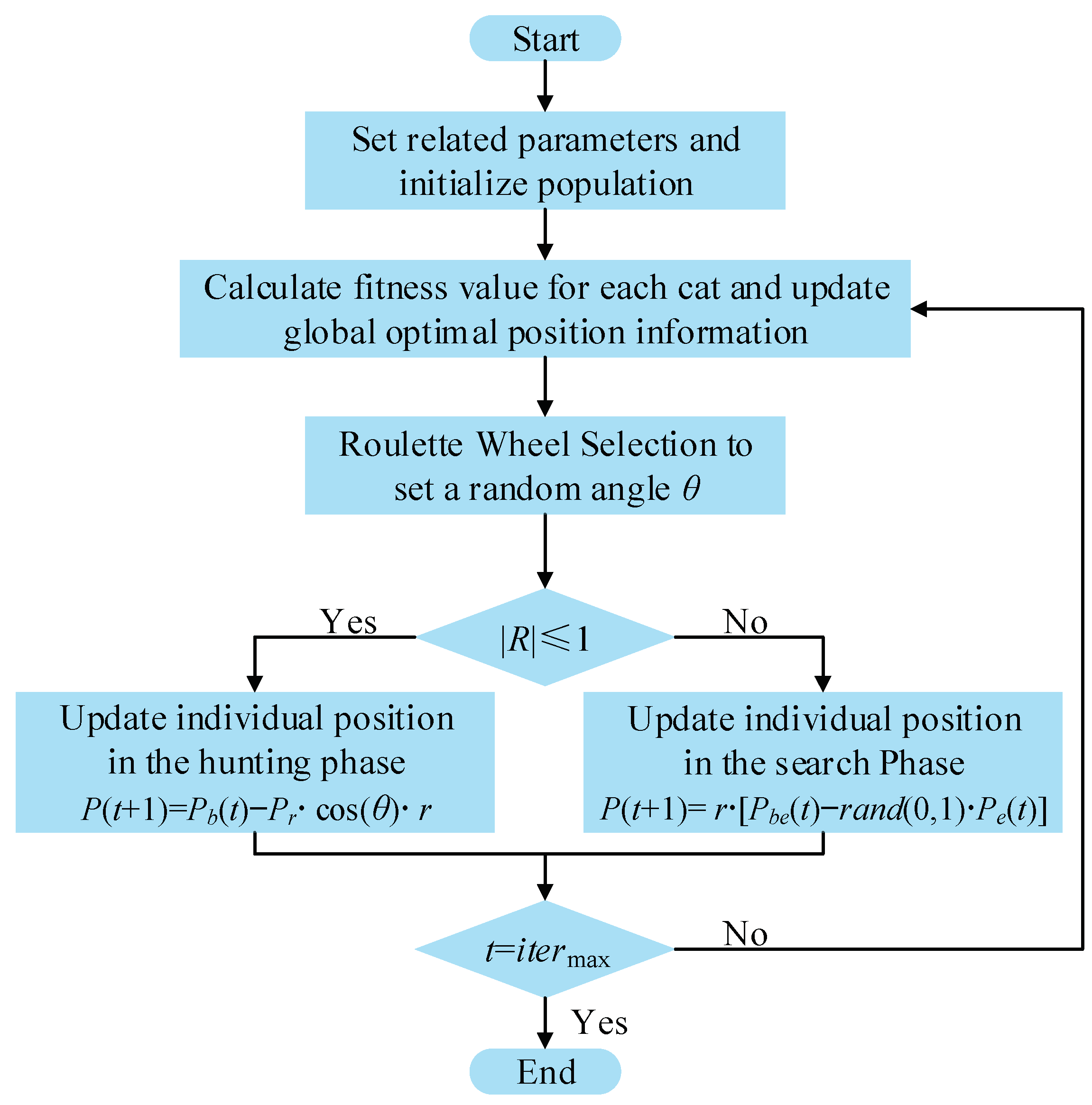
2.3. Optimizing VMD Parameters Using SCSO Algorithm

SCSO is a novel metaheuristic optimization method inspired by the predatory behavior of sand cats. In the wild, sand cats can detect low frequencies below 2 kHz, which helps them capture prey from long distances in short periods. The algorithm balances global and local search, effectively avoiding local extrema and achieving higher convergence accuracy and faster speed. Moreover, the SCSO algorithm requires fewer parameters; therefore, it is simpler to implement. Compared to widely used algorithms such as particle swarm algorithm, whale optimization algorithm, and grey wolf optimization algorithm, SCSO demonstrates higher computational efficiency and superior convergence performance. This makes it suitable for solving complex optimization problems with fewer resources in a shorter time. The specifics of this algorithm have been effectively validated in the literature [35]. Finally, the mathematical model for the sand cat population search is formulated below.

The SCSO algorithm introduces the auditory sensitivity parameter r_G, which decreases linearly from two to zero over iterations. This aids the sand cats in gradually approaching their prey without losing or skipping past it. Moreover, the parameter r represents the sensitivity range of each sand cat, aiding in the avoidance of local optima. Therefore, the specific formulas are given in Equations (7) and (8).

$$r_G=s_{\mathrm{M}}-\left({\displaystyle \frac{s_{\mathrm{M}}\times t}{ite{r}_{\max }}}\right)$$

(7)

$$r=r_G\times rand(0,1)$$

(8)

where S_M represents the auditory characteristics of sand cats with a default value of two, iter_max denotes the maximum number of iterations, and t indicates the current iteration.

In the population position updating mechanism, the algorithm emulates the searching and hunting behaviors of sand cats. The transition between both stages is governed by the parameter R, expressed in Equation (9).

$$R=2\times r_{\mathrm{G}}\times rand(0,1)-r_{\mathrm{G}}$$

(9)

When |R| > 1, the sand cat enters the search phase. In iteration t + 1, the position of each cat will be dynamically updated according to the optimal position P_bc(t), current position P_c(t), and auditory sensitivity r. This can be denoted by Equation (10).

$$P(t+1)=r\cdot [P_{bc}\left(t\right)-rand(0,1)\cdot P_c\left(t\right)]$$

(10)

When |R| ≤ 1, the sand cat is built to hunt the target prey. Moreover, referring to Equation (11), P_r represents a random position generated by the optimal position P_b(t) and the current one P_c(t). Assuming that the sensitivity range of the sand cat is a circle, SCSO selects a random angle θ for each sand cat to approach the prey to avoid falling into a local optimum. Therefore, the specific equations are defined as follows:

$$P_r=|rand(0,1)\cdot P_b(t)-P_c(t)|$$

(11)

$$P(t+1)=P_b(t)-P_r\cdot \cos (\theta )\cdot r$$

(12)

where the prey position serves as the problem to be optimized, i.e., the average permutation entropy of the objective function of Equation (6). The sand cat position represents the solution to the problem, namely the decomposition modal number K and the penalty factor α.

The specific flow of the SCSO algorithm is shown in Figure 2. The SCSO algorithm optimizes key parameters of the VMD, generating the set of IMFs with the smallest average permutation entropy and the highest regularity; thus, reducing the prediction difficulty of the model.

3. Load Forecasting Model Combining TCN and BiLSTM

3.1. Temporal Convolutional Network (TCN)

TCN is a novel CNN architecture used for time series data. However, CNN employs a conventional convolutional layer with a restricted receptive field. To expand the receptive field, increasing the network depth is typically required. However, this increase leads to unstable network operations. To address these challenges, TCN integrates expansion causal convolution and residual modules based on the CNN model [36]. By introducing a dilation factor, the dilated causal convolution layer effectively performs interval sampling of input data and expands the receptive field. As the neural network deepens, blindly stacking convolutional layers can negatively affect the stability of the network performance. The residual modules in TCN enable information to be transferred from layer to layer, allowing the network to maintain depth while effectively mitigating challenges including vanishing or exploding gradients.

Figure 3 shows the specifics of the residual modules. Each residual block contains two layers of the dilated causal convolution, with WeightNorm, Dropout, and ReLU present in every residual block. The dilated causal convolution layer extracts hidden features from the input. A rectified linear unit (ReLU) activation function is included to avoid gradient vanishing. Moreover, WeightNorm and Dropout layers are used for regularization to prevent overfitting. Finally, the residual block employs a 1 × 1 convolution to guarantee that the input and output dimensions match.

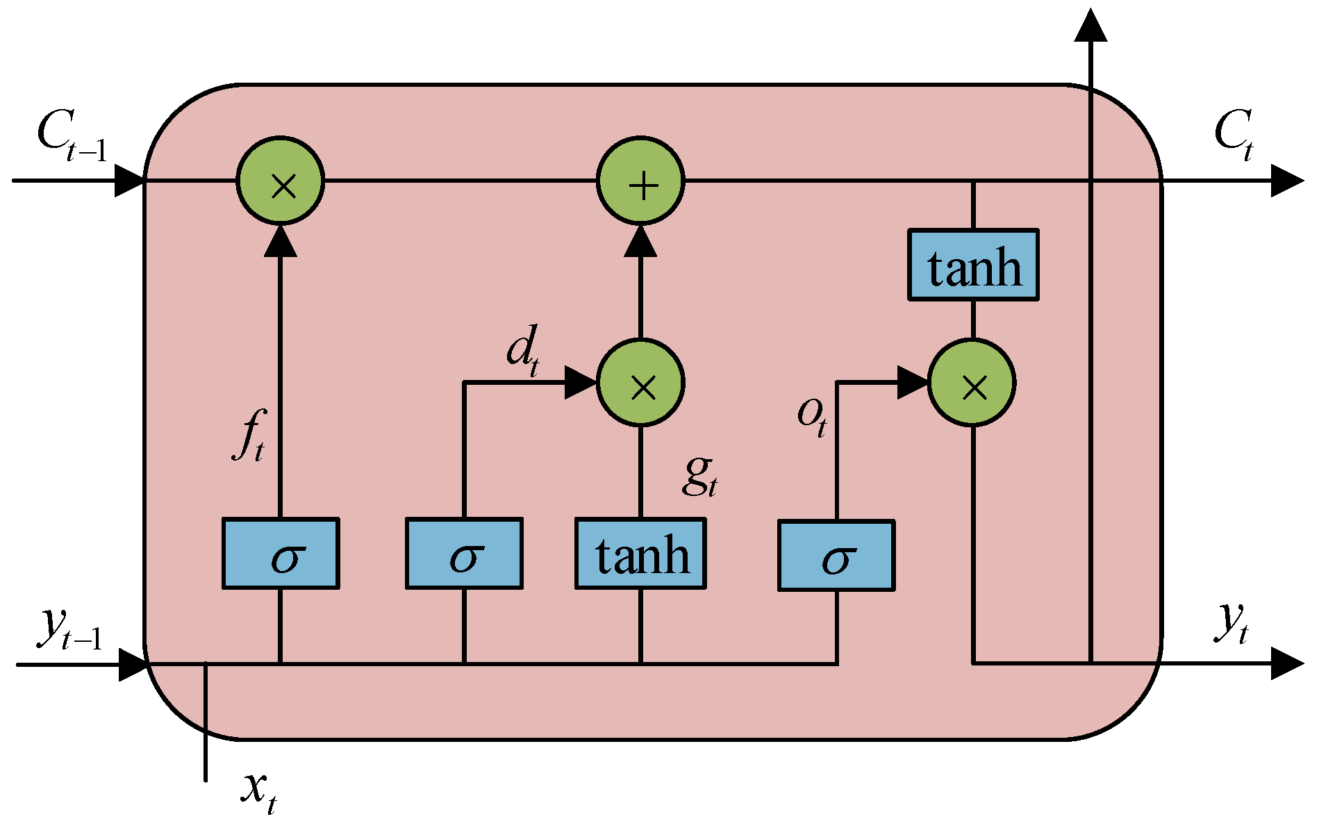
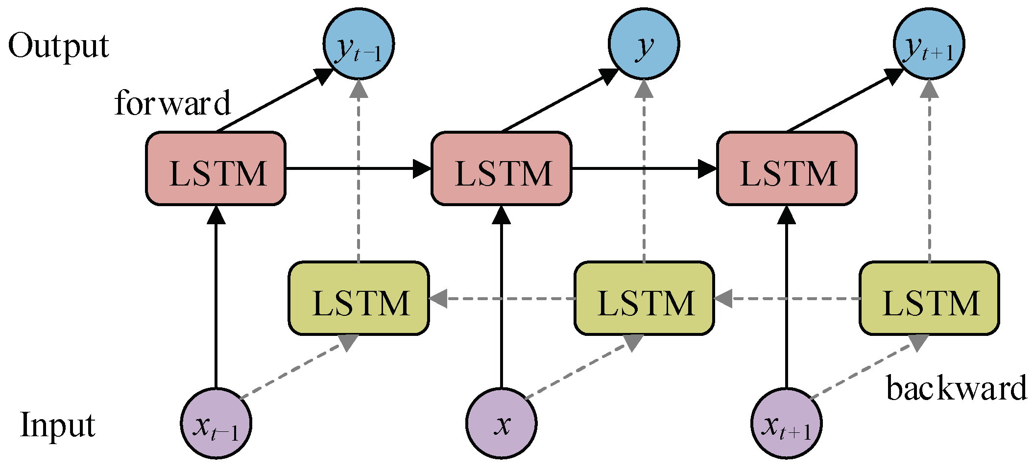
3.2. Bidirectional Long Short-Term Memory Network

LSTM is an advanced technique adapted from the Recurrent Neural Network (RNN) that introduces gate structures to regulate information updating and forgetting. This feature allows for the effective capture of long-term dependencies on time series data [37]. The LSTM network structure is shown in Figure 4 where the input at the current time t consists of three components: the state information C_t−1 and the output y_t−1 from the previous time step, along with the current input x_t. As for the output at the current time t, it includes two parts: the state information C_t and the output y_t of the current time. Therefore, the equations of LSTM are expressed as follows:

$$f_t=\sigma (W_{fx}{x}_t+W_{fy}{y}_{t-1}+b_f)$$

(13)

$$d_t=\sigma (W_{dx}{x}_t+W_{dy}{y}_{t-1}+b_d)$$

(14)

$$g_t=\tanh (W_{gx}{x}_t+W_{gy}{y}_{t-1}+b_g)$$

(15)

$$o_t=\sigma (W_{ox}{x}_t+W_{oy}{y}_{t-1}+b_o)$$

(16)

$$C_t=g_t{d}_t+C_{t-1}{f}_t$$

(17)

$$y_t=\tanh (C_t)o_t$$

(18)

where f_t represents the output of the forgetting gate, d_t denotes the output of the input gate, and o_t indicates the output of the output gate. Furthermore, W is the weight matrix while b is bias matrix. Moreover, functions σ and tanh represent the sigmoid activation and the tangent hyperbolic activation functions, respectively.

The standard LSTM model can only learn and train unidirectionally on time series data, leading to low data utilization efficiency. In contrast, BiLSTM [38] utilizes a bidirectional data sequence processing technique, enabling it to comprehensively consider both the forward and backward resources of time series data, thereby uncovering intrinsic connections between each moment and both past and future moments. Although GRU also possesses a gate structure mechanism, its simpler structure results in low flexibility. However, BiLSTM has independent input and forgetting gates that can better control the process of forgetting and updating information, making it suitable for highly volatile and interdependent multi-energy load sequences. In BiLSTM, the same sequence of information is fed into two LSTM structures operating in opposite directions for feature extraction. The outputs of these two structures are then combined according to certain weights to obtain the final output of the BiLSTM network, and its structure is displayed in Figure 5.

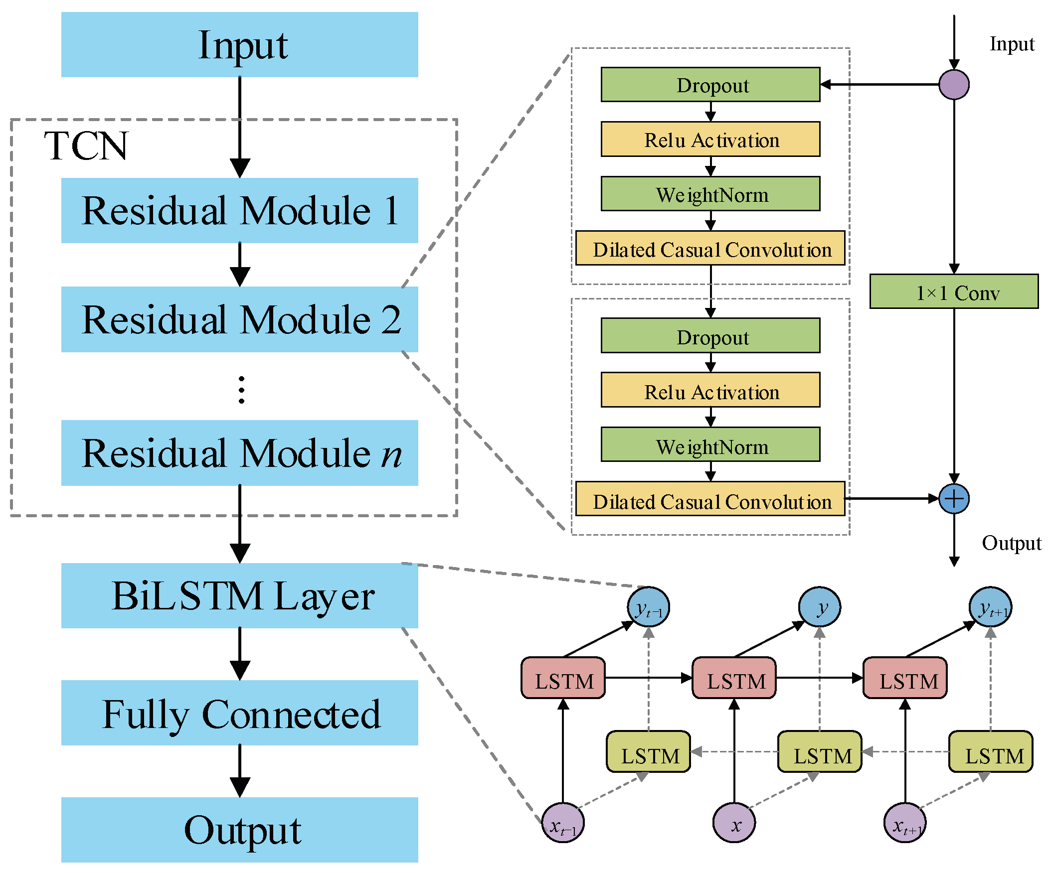
3.3. TCN-BiLSTM Neural Network

The combined TCN-BiLSTM model synthesizes the advantages of both TCN and BiLSTM. The structure of the combined model is displayed in Figure 6. Initially, the sample data are inputted into the TCN, where dilated causal convolution and residual modules are used to extract features from the input data. Consequently, extracted features are transmitted to the BiLSTM network. The intrinsic regularities and trends among data are captured by the BiLSTM bidirectional structure; therefore, predicting future data points. Ultimately, the fully connected layer generates the predicted values. Moreover, the TCN-BiLSTM network can comprehensively extract the hidden features from the time series data, effectively learn complex dependencies, and display strong time series data prediction capabilities.

4. Multi-Energy Load Forecasting Method Using VMD-TCN-BiLSTM

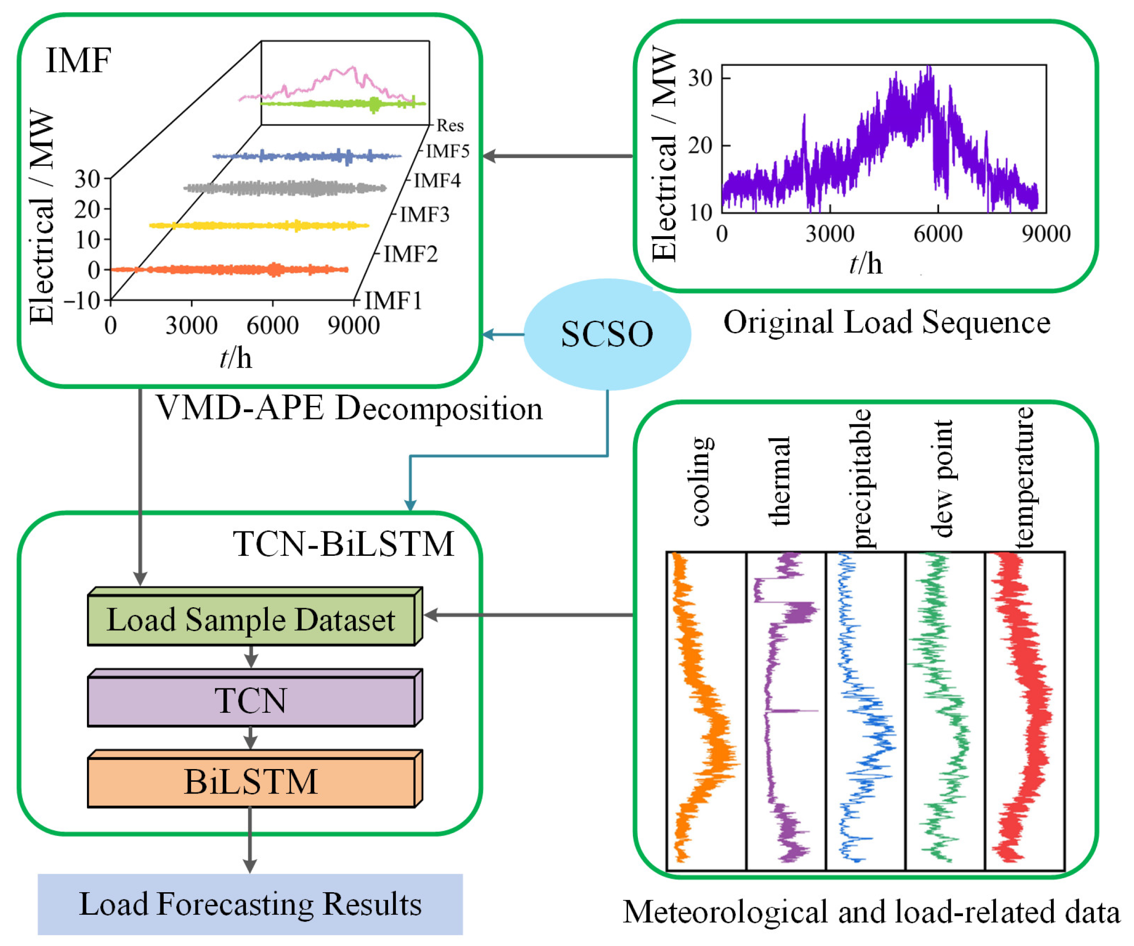
4.1. Forecasting Process

By integrating the VMD, PE, TCN, and BiLSTM algorithms, the IES multi-energy load forecasting model is built as shown in Figure 7. The detailed steps are represented as follows:

(1)

To address the non-stationary characteristics of the multi-variate load sequence, this study builds a VMD optimization model based on the minimum average permutation entropy (VMD-APE). The SCSO algorithm is employed to solve this model, generating the IMF sets as well as the residues for electrical, thermal, and cooling loads. Therefore, it facilitates the effective decomposition of the multivariate loads;

(2)

The preprocessed multi-variate load IMF sets are combined with the meteorological information and related load data to build the input and output samples for electrical, thermal, and cooling loads;

(3)

The TCN-BiLSTM models are constructed for different types of loads and used to learn and train the sample sequences. Parameters’ optimization is achieved using the SCSO algorithm;

(4)

Trained models are then used for multi-variate load forecasting. Evaluation metrics are developed to assess forecasting accuracy.

4.2. Evaluation Metrics

To accurately assess the load forecasting model performance, this paper selects the following two indicators: Mean Absolute Percentage Error (E_MAPE) and Coefficient of Determination (R²). They are calculated as follows:

$$R^2=1-{\displaystyle \frac{{\displaystyle \sum _{t=1}^{\rho }}{({\widehat{y}}_t-y_t)}^2}{{\displaystyle \sum _{t=1}^{\rho }}{({\overline{y}}_t-y_t)}^2}}$$

(19)

$$E_{\mathrm{MAPE}}={\displaystyle \frac{1}{\rho }}{\displaystyle \sum _{t=1}^{\rho }}{\displaystyle \frac{\left|y_t-{\widehat{y}}_t\right|}{y_t}}\times 100\%$$

(20)

where y_t and ${\widehat{y}}_t$ are the actual and predicted load values at time t, ${\overline{y}}_t$ represents the average value of y_t, and ρ denotes the length of the predicted data.

Moreover, R² assesses the correlation between the predicted and observed values. The closer R² value is to the unit, the better the model will fit. As for E_MAPE, it reflects the relative deviation magnitude between the predicted and actual values. It is worth noting that the smaller the E_MAPE value is, the more accurate the prediction will be.

5. Empirical Studies

This study utilizes the historical dataset from the Arizona State University Tempe campus [39,40] to perform an empirical analysis, focusing on electrical, thermal, and cooling energy data. Moreover, the IES dataset spans from January 2022 to December 2022, with a sampling frequency set to one hour, yielding 8760 load data points. It is important to mention that data from December 2022 was designated as the test set, with the remaining data divided into training and validation sets using an 8:2 ratio and a forecast step of one hour in the short term. In addition, local meteorological data were generated by the National Solar Radiation Database [41], and it includes several parameters such as temperature, dew point, and precipitation.

5.1. Load Series Decomposition

To elevate the precision of IES’s multi-energy load forecasting and alleviate the adverse effects of nonlinear features on predictions, a load decomposition model, based on PE and VMD, is developed in this work. The SCSO algorithm is employed to define the decomposition modal numbers K as well as the penalty factors α for electrical, thermal, and cooling loads, where K are 5, 3, and 5, and α are 2724, 2468, and 2997, respectively. The IMF components obtained from the VMD of the multi-energy load are illustrated in Figure 8.

To verify the critical role of K and α in VMD, the average permutation entropy is used to evaluate the decomposition effect.

Table 1. APE values for VMD of electric load under different K and α.

	K = 2	K = 3	K = 4	K = 5	K = 6	K = 7	K = 8
α = 100	0.984	0.979	0.924	0.927	0.939	0.921	0.906
α = 500	0.973	0.938	0.910	0.933	0.923	0.903	0.916
α = 1000	0.938	0.938	0.917	0.903	0.906	0.890	0.899
α = 2000	0.911	0.889	0.904	0.870	0.894	0.900	0.922
α = 2724	0.920	0.932	0.911	0.859	0.879	0.929	0.916
α = 3000	0.924	0.928	0.908	0.880	0.876	0.921	0.926

lists the calculation result of the electrical load’s APE under different K and α, shown as normalized values. When α is maintained constant, APE decreases significantly as K increases, which confirms VMD’s ability to reduce signal complexity. However, when α is a large value, it further increases K leads to greater complexity of the decomposition result. Moreover, Table 1 also displays that APE reaches a minimum value of 0.859 when K and α are set as the optimization outcomes of SCSO, namely K = 5 and α = 2724. At this point, the subsequence complexity is at its lowest, which ensures the rational selection of VMD parameters.

5.2. Input and Output Feature Selection

Input features are key factors affecting load forecasting results. Thus, the selection of input features with robust correlation to the load is paramount to enhance the precision of predicting future alterations in multiple loads. Generally, factors that significantly influence load encompass both historical load and meteorological data [42]. Based on existing data, this work considers that the load changes strongly correlate with the recent historical data. Due to the variability and coupling among different load types [43], input features selection contains their own historical load data and other related coupling load data. Moreover, there is a high correlation between load and meteorological data, particularly when it comes to a multi-energy system’s cooling and thermal load. Therefore, temperature, dew point, and precipitation are considered as input features. To sum up,

Table 2. Input and output features for electric load forecasting model.

Input Feature	Output Feature
Electrical load IMFs in the previous five hours	Electricity load to be forecast at the moment
Thermal and cooling load in the previous five hours
Temperature, dew point, precipitable

displays the chosen input features for the electrical load.

5.3. Hyper-Parameters Description of TCN-BiLSTM

Considering the distinct characteristics of electrical, thermal, and cooling load sequences, separate TCN-BiLSTM forecasting models are constructed for each load type and their parameters are configured. The specific structure of the combined neural network model is as follows: TCN consists of three layers of residual modules, while BiLSTM comprises a single hidden layer unit. The SCSO algorithm is utilized to optimize four key parameters: the number of convolutional kernels; the hidden layer units; the learning rate; and the regularization coefficient. E_MAPE represents the fitness function for SCSO, with a population size of 30 and running for 50 iterations. The specific parameter settings for the TCN-BiLSTM forecasting models are detailed in

Table 3. Parameter setting of TCN-BiLSTM model.

Parameter	Value Range
Convolution layer kernel size	3
Dilation factors	1/2/4
Number of convolution layer kernels	[8, 64]
Hidden layer units in BiLSTM layer	[10, 100]
Learning rate	[1 × 10−4, 1 × 10−1]
Regularization coefficient	[1 × 10−4, 1 × 10−1]

.

5.4. Comparison of Different Decomposition Methods

To demonstrate the superiority of the proposed VMD-APE decomposition method, experiments are conducted using the no-modal decomposition and CEEMDAN for comparison purposes. Moreover, the TCN-BiLSTM model is utilized to predict the test set separately. The prediction results are displayed in

Table 4. Metrics of different load decomposition methods for load forecasting.

Load Type	Decomposition Methods	R2	EMAPE/%
Electrical	No decomposition	0.742	4.145
	CEEMDAN	0.952	1.833
	VMD-APE	0.963	1.462
Thermal	No decomposition	0.880	4.153
	CEEMDAN	0.889	4.888
	VMD-APE	0.985	1.563
Cooling	No decomposition	0.935	5.739
	CEEMDAN	0.987	2.525
	VMD-APE	0.993	1.830

. Compared to no-modal decomposition, E_MAPE metrics for electrical and cooling loads using the CEEMDAN method are reduced by 55.778% and 56.003%, respectively, whereas the prediction accuracy is almost doubled. However, the prediction accuracy for thermal loads does not improve but decreases instead. The optimal prediction findings are achieved using the VMD-APE modal decomposition. Compared to no-modal decomposition, the E_MAPE of electrical, thermal, and cooling loads decreased, respectively, by 64.729%, 62.365%, and 68.113% with corresponding improvements of R² by 29.784%, 11.932%, and 6.203%. These evaluation metrics demonstrate superior performance compared to other load decomposition methods.

Owing to the strong nonlinear characteristics of IES multi-energy loads, direct prediction without decomposition leads to suboptimal accuracy. Although CEEMDAN can improve prediction accuracy up to a point, it suffers from modal aliasing problems that compromise its precision, making it unsuitable for all signal decomposition tasks. Therefore, the proposed VMD-APE decomposition method diminishes the complexity and volatility of the original load sequence, effectively reducing the prediction difficulty. This enhances the accuracy of the TCN-BiLSTM model’s prediction, thereby validating the effectiveness of the proposed load decomposition method.

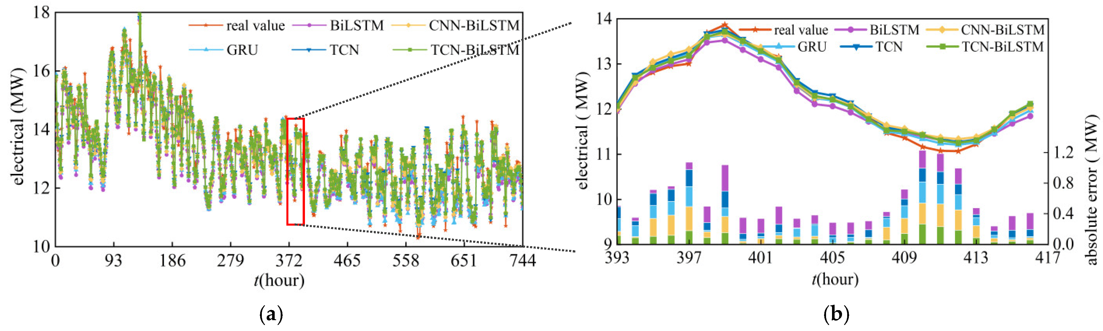
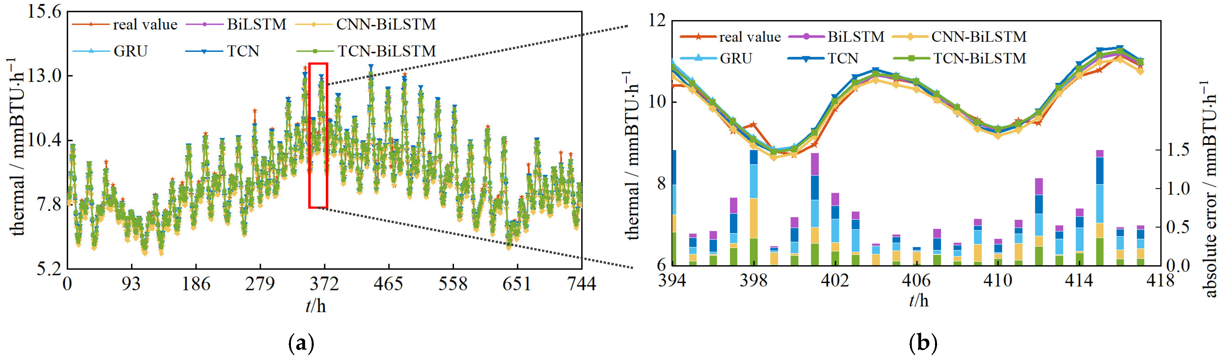
5.5. Comparison of Different Forecasting Models

To validate the accuracy of the proposed prediction model, load forecasting and comparative analysis are conducted using existing individual models such as BiLSTM, GRU, and TCN, as well as existing hybrid models such as CNN-BiLSTM, against the proposed TCN-BiLSTM hybrid model. VMD-APE method was used to decompose the original load sequence. Each prediction model applied the SCSO algorithm for hyper-parameter selection to ensure the fairness of the experiments.

To intuitively present the prediction results, 24 consecutive hours of predictions were selected from the test set’s prediction curves for localized zoom, with absolute errors stacked at the same sampling points for supplementary illustration. The larger the stacked area is, the greater the absolute error of the model will be. The prediction results and corresponding error stacking plots for various models are illustrated in Figure 9, Figure 10 and Figure 11. The green curve represents the predicted values of the combined TCN-BiLSTM model, while the red one denotes the actual measured values of the load. It is evident that, compared to other existing load prediction models, the TCN-BiLSTM model exhibits the smallest error area and the best fitting between the prediction curve and the actual values.

The evaluation metrics of the prediction results of different models on the test set are displayed in

Table 5. Metrics for Different Forecasting Models.

Load Type	Prediction Model	R2	EMAPE/%
Electrical	BiLSTM	0.944	1.939
	TCN	0.961	1.551
	GRU	0.960	1.544
	CNN-BiLSM	0.959	1.533
	TCN-BiLSM	0.963	1.462
Thermal	BiLSTM	0.983	1.637
	TCN	0.979	1.883
	GRU	0.983	1.655
	CNN-BiLSM	0.971	2.269
	TCN-BiLSM	0.985	1.563
Cooling	BiLSTM	0.986	2.648
	TCN	0.992	1.838
	GRU	0.989	2.317
	CNN-BiLSM	0.988	2.289
	TCN-BiLSM	0.993	1.830

. The E_MAPE metrics of the TCN-BiLSTM model are 1.462%, 1.563%, and 1.830% for electrical, thermal, and cooling loads, respectively. Meanwhile, the R² metrics are 0.963, 0.985, and 0.993, respectively. Both metrics overpass those of any existing individual models, such as BiLSTM, GRU, and TCN. Moreover, compared to the existing CNN-BiLSTM model, the TCN-BiLSTM model’s E_MAPE indices for electrical, thermal, and cooling loads decrease by 4.631%, 31.115%, and 20.052%, respectively, significantly improving prediction accuracy.

The standard CNN employs a conventional convolutional layer with a limited receptive field. As the network depth deepens, CNN encounters gradient vanishing and exploding issues, which compromise model training stability. In contrast, TCN integrates dilated causal convolution and residual modules to expand the receptive field while maintaining the network depth. This design enables the network to effectively capture long-term dependencies in time series data. Moreover, BiLSTM employs a bidirectional data processing technique, allowing for a comprehensive exploration of the inherent relationship among data. Although GRU also has gate structure mechanisms, BiLSTM’s independent input and forget gates offer greater flexibility and demonstrate superior performance in handling complex time series data. To sum up, the TCN-BiLSTM model integrates the advantages of individual prediction models, such as TCN and BiLSTM, offering higher accurate prediction results and better applicability for multi-energy load forecasting in IES.

6. Conclusions

By synthesizing the nonlinearity and coupling of multi-energy loads, including electrical, thermal, and cooling loads, this study proposes a novel multi-energy load forecasting model based on the VMD-TCN-BiLSTM method. A mathematical model is developed to optimize the multi-energy load VMD parameters based on the minimum average PE. Then, the load sequence is decomposed into different IMFs using VMD-APE. Compared to other load decomposition methods, the proposed method efficiently reduces load sequence complexity and yields better prediction performance. Added to that, a multi-energy load forecasting model network structure combining TCN and BiLSTM is designed. TCN captures load data characteristics while BiLSTM identifies load sequences’ forward and backward trends for prediction. The SCSO algorithm is utilized to optimize the model’s hyper-parameters to generate the optimal prediction model, significantly improving its prediction accuracy. The findings demonstrate that the evaluation indices of the VMD-TCN-BiLSTM hybrid model forecasting results surpass those of individual models, such as BiLSTM, GRU, and TCN, as well as the existing hybrid models like CNN-BiLSTM.

Although the findings of this research can provide a reference for multi-energy load forecasting in IES, it still has some shortcomings. The next step consists of further exploring the applicability of the prediction model to datasets with different features. Furthermore, the optimization algorithm possesses the potential for enhancement in terms of convergence velocity. In the forthcoming work, we will increase the prediction model’s overall performance by expanding the model and improving the algorithm, thereby implementing the model’s practicality.

References

1. Ji, L.; Zhang, B.B.; Huang, G.H.; Xie, Y.L.; Niu, D.X. GHG-mitigation oriented and coal-consumption constrained inexact robust model for regional energy structure adjustment-A case study for Jiangsu Province, China. Renew. Energy 2018, 123, 549–562. [Google Scholar] [CrossRef]
2. Xie, B.C.; Zhang, R.Y.; Chen, X.P. China’s optimal development pathway of intermittent renewable power towards carbon neutrality. J. Clean. Prod. 2023, 406, 136903. [Google Scholar] [CrossRef]
3. Xu, M.K.; Liao, C.P.; Huang, Y.; Gao, X.Q.; Dong, G.L.; Liu, Z. LEAP model-based analysis to low-carbon transformation path in the power sector: A case study of Guangdong-Hong Kong-Macao Greater Bay Area. Sci. Rep. 2024, 14, 7405. [Google Scholar] [CrossRef] [PubMed]
4. Niu, D.X.; Yu, M.; Sun, L.J.; Gao, T.; Wang, K.K. Short-term multi-energy load forecasting for integrated energy systems based on CNN-BiGRU optimized by attention mechanism. Appl. Energy 2022, 313, 118801. [Google Scholar] [CrossRef]
5. Talaat, M.; Tayseer, M.; Farahat, M.A.; Song, D.R. Artificial intelligence strategies for simulating the integrated energy systems. Artif. Intell. Rev. 2024, 57, 106. [Google Scholar] [CrossRef]
6. Wang, J.X.; Zhong, H.W.; Ma, Z.M.; Xia, Q.; Kang, C.Q. Review and prospect of integrated demand response in the multi-energy system. Appl. Energy 2017, 202, 772–782. [Google Scholar] [CrossRef]
7. Dal Cin, E.; Carraro, G.; Lazzaretto, A.; Tsatsaronis, G. Optimizing the retrofit design and operation of multi-energy systems integrated with energy networks. J. Energy Resour. Technol. 2024, 146, 042102. [Google Scholar] [CrossRef]
8. Wang, Y.L.; Qin, Y.M.; Ma, Z.B.; Wang, Y.N.; Li, Y. Operation optimisation of integrated energy systems based on cooperative game with hydrogen energy storage systems. Int. J. Hydrogen Energy 2023, 48, 37335–37354. [Google Scholar] [CrossRef]
9. Li, K.; Mu, Y.C.; Yang, F.; Wang, H.Y.; Yan, Y.; Zhang, C.H. A novel short-term multi-energy load forecasting method for integrated energy system based on feature separation-fusion technology and improved CNN. Appl. Energy 2023, 351, 121823. [Google Scholar] [CrossRef]
10. Liu, B.D.; Nowotarski, J.; Hong, T.; Weron, R. Probabilistic load forecasting via quantile regression averaging on sister forecasts. IEEE Trans. Smart Grid 2017, 8, 730–737. [Google Scholar] [CrossRef]
11. Laouafi, A.; Mordjaoui, M.; Laouafi, F.; Boukelia, T.E. Daily peak electricity demand forecasting based on an adaptive hybrid two-stage methodology. Int. J. Electr. Power Energy Syst. 2016, 77, 136–144. [Google Scholar] [CrossRef]
12. Tarmanini, C.; Sarma, N.; Gezegin, C.; Ozgonenel, O. Short term load forecasting based on ARIMA and ANN approaches. Energy Rep. 2023, 9, 550–557. [Google Scholar] [CrossRef]
13. Fang, P.; Fu, W.L.; Wang, K.; Xiong, D.Z.; Zhang, K. A compositive architecture coupling outlier correction, EWT, nonlinear Volterra multi-model fusion with multi-objective optimization for short-term wind speed forecasting. Appl. Energy 2022, 307, 118191. [Google Scholar] [CrossRef]
14. Jahani, A.; Zare, K.; Khanli, L.M. Short-term load forecasting for microgrid energy management system using hybrid SPM-LSTM. Sustain. Cities Soc. 2023, 98, 104775. [Google Scholar] [CrossRef]
15. Eskandari, H.; Imani, M.; Moghaddam, M.P. Best-tree wavelet packet transform bidirectional GRU for short-term load forecasting. J. Supercomput. 2023, 79, 13545–13577. [Google Scholar] [CrossRef]
16. Wang, Y.Y.; Chen, J.; Chen, X.Q.; Zeng, X.J.; Kong, Y.; Sun, S.F.; Guo, Y.S.; Liu, Y. Short-term load forecasting for industrial customers based on TCN-LightGBM. IEEE Trans. Power Syst. 2021, 36, 1984–1997. [Google Scholar] [CrossRef]
17. Cai, C.C.; Li, Y.J.; Su, Z.H.; Zhu, T.Q.; He, Y.Y. Short-term electrical load forecasting based on VMD and GRU-TCN hybrid network. Appl. Sci. 2022, 12, 6647. [Google Scholar] [CrossRef]
18. Sulandari, W.; Subanar; Lee, M.H.; Rodrigues, P.C. Indonesian electricity load forecasting using singular spectrum analysis, fuzzy systems and neural networks. Energy 2020, 190, 116408. [Google Scholar] [CrossRef]
19. Wang, L.Y.; Zhou, X.; Xu, H.L.; Tian, T.; Tong, H.M. Short-term electrical load forecasting model based on multi-dimensional meteorological information spatio-temporal fusion and optimized variational mode decomposition. IET Gener. Transm. Distrib. 2023, 17, 4647–4663. [Google Scholar] [CrossRef]
20. Ran, P.; Dong, K.; Liu, X.; Wang, J. Short-term load forecasting based on CEEMDAN and Transformer. Electr. Power Syst. Res. 2023, 214, 108885. [Google Scholar] [CrossRef]
21. Bedi, J.; Toshniwal, D. Energy load time-series forecast using decomposition and autoencoder integrated memory network. Appl. Soft Comput. 2020, 93, 106390. [Google Scholar] [CrossRef]
22. Hu, X.; Li, K.Y.; Li, J.F.; Zhong, T.T.; Wu, W.N.; Zhang, X.; Feng, W.J. Load forecasting model consisting of data mining based orthogonal greedy algorithm and long short-term memory network. Energy Rep. 2022, 8, 235–242. [Google Scholar] [CrossRef]
23. Sekhar, C.; Dahiya, R. Robust framework based on hybrid deep learning approach for short term load forecasting of building electricity demand. Energy 2023, 268, 126660. [Google Scholar] [CrossRef]
24. Ma, S.J.; Ning, J.; Mao, N.; Liu, J.; Shi, R.F. Research on Machine Learning-Based method for predicting industrial park electric vehicle charging load. Sustainability 2024, 16, 7258. [Google Scholar] [CrossRef]
25. Xiao, Z.C.; Yu, L.J.; Zhang, H.J.; Zhang, X.T.; Su, Y.X. HVAC load forecasting based on the CEEMDAN-Conv1D-BiLSTM-AM model. Mathematics 2023, 11, 4630. [Google Scholar] [CrossRef]
26. Liu, M.P.; Sun, X.H.; Wang, Q.N.; Deng, S.H. Short-term load forecasting using EMD with feature selection and TCN-based deep learning model. Energies 2022, 15, 7170. [Google Scholar] [CrossRef]
27. Hong, Y.; Wang, D.; Su, J.M.; Ren, M.W.; Xu, W.Q.; Wei, Y.H.; Yang, Z. Short-Term Power Load Forecasting in Three Stages Based on CEEMDAN-TGA Model. Sustainability 2023, 15, 11123. [Google Scholar] [CrossRef]
28. Jia, T.R.; Yao, L.X.; Yang, G.Q.; He, Q. A short-term power load forecasting method of based on the CEEMDAN-MVO-GRU. Sustainability 2022, 14, 16460. [Google Scholar] [CrossRef]
29. Li, K.; Huang, W.; Hu, G.Y.; Li, J. Ultra-short term power load forecasting based on CEEMDAN-SE and LSTM neural network. Energy Build. 2023, 279, 112666. [Google Scholar] [CrossRef]
30. Wen, Y.; Pan, S.; Li, X.X.; Li, Z.B. Highly fluctuating short-term load forecasting based on improved secondary decomposition and optimized VMD. Sustain. Energy Grids Netw. 2024, 37, 101270. [Google Scholar] [CrossRef]
31. Li, W.W.; Shi, Q.; Sibtain, M.; Li, D.; Mbanze, D.E. A hybrid forecasting model for short-term power load based on sample entropy, two-phase decomposition and whale algorithm optimized support vector regression. IEEE Access 2020, 8, 166907–166921. [Google Scholar] [CrossRef]
32. Chen, G.; Ma, X.F.; Lin, W. Multifeature-based Variational Mode Decomposition-Temporal Convolutional Network-Long Short-Term Memory for short-term forecasting of the load of port power systems. Sustainability 2024, 164, 5321. [Google Scholar] [CrossRef]
33. Dragomiretskiy, K.; Zosso, D. Variational mode decomposition. IEEE Trans. Signal Process. 2014, 62, 531–544. [Google Scholar] [CrossRef]
34. Keller, K.; Mangold, T.; Stolz, I.; Werner, J. Permutation entropy: New ideas and challenges. Entropy 2017, 19, 134. [Google Scholar] [CrossRef]
35. Seyyedabbasi, A.; Kiani, F. Sand Cat swarm optimization: A nature-inspired algorithm to solve global optimization problems. Eng. Comput. 2023, 39, 2627–2651. [Google Scholar] [CrossRef]
36. Lin, Q.Y.; Yang, Z.P.; Huang, J.; Deng, J.; Chen, L.; Zhang, Y.R. A Landslide Displacement Prediction Model Based on the ICEEMDAN Method and the TCN-BiLSTM Combined Neural Network. Water 2023, 15, 4247. [Google Scholar] [CrossRef]
37. Hochreiter, S.; Schmidhuber, J. Long short-term memory. Neural Comput. 1997, 9, 1735–1780. [Google Scholar] [CrossRef]
38. Xia, T.B.; Song, Y.; Zheng, Y.; Pan, E.S.; Xi, L.F. An ensemble framework based on convolutional bi-directional LSTM with multiple time windows for remaining useful life estimation. Comput. Ind. 2020, 115, 103182. [Google Scholar] [CrossRef]
39. AUS. Campus Metabolism. Available online: https://www.asu.edu/ (accessed on 5 January 2023).
40. Fan, J.L.; Zhuang, W.; Xia, M.; Fang, W.X.; Liu, J. Optimizing attention in a Transformer for multihorizon, multienergy load forecasting in integrated energy systems. IEEE Trans. Ind. Inform. 2024, 20, 10238–10248. [Google Scholar] [CrossRef]
41. NSRDB. Data Viewer. Available online: https://nsrdb.nrel.gov/data-viewer (accessed on 6 January 2023).
42. Wang, C.; Wang, Y.; Ding, Z.T.; Zheng, T.; Hu, J.Y.; Zhang, K.F. A transformer-based method of multienergy load forecasting in integrated energy system. IEEE Trans. Smart Grid 2022, 13, 2703–2714. [Google Scholar] [CrossRef]
43. Guo, Y.X.; Li, Y.; Qiao, X.B.; Zhang, Z.Y.; Zhou, W.F.; Mei, Y.J.; Lin, J.J.; Zhou, Y.C.; Nakanishi, Y. BiLSTM multitask learning-based combined load forecasting considering the loads coupling relationship for multienergy system. IEEE Trans. Smart Grid 2022, 13, 3481–3492. [Google Scholar] [CrossRef]
Figure 1. Research progress of deep learning techniques in the field of load forecasting.
Sustainability 16 10082 g001
Figure 2. Flowchart of the Sand Cat Swarm Optimization algorithm.
Sustainability 16 10082 g002
Figure 3. Network structure of TCN model.
Sustainability 16 10082 g003
Figure 4. Network structure of LSTM.
Sustainability 16 10082 g004
Figure 5. Network structure of BiLSTM.
Sustainability 16 10082 g005
Figure 6. Network structure of TCN-BiLSTM.
Sustainability 16 10082 g006
Figure 7. A multi-energy load forecasting flowchart based on VMD-TCN-BiLSTM.
Sustainability 16 10082 g007
Figure 8. VMD results. (a) Electric load, (b) Cooling load, (c) Thermal load.
Sustainability 16 10082 g008
Figure 9. Electrical load forecasting results. (a) Electrical load forecasting results of single and combined model. (b) Local magnification of result.
Sustainability 16 10082 g009
Figure 10. Thermal load forecasting results. (a) Thermal load forecasting results of single and combined model. (b) Local magnification of result.
Sustainability 16 10082 g010
Figure 11. Cooling load forecasting results. (a) Cooling load forecasting results of single and combined model. (b) Local magnification of result.
Sustainability 16 10082 g011