
Effects of Heavy Grazing on Interspecific Relationships at Different Spatial Scales in Desert Steppe of China


Abstract
:1. Introduction
2. Materials and Methods
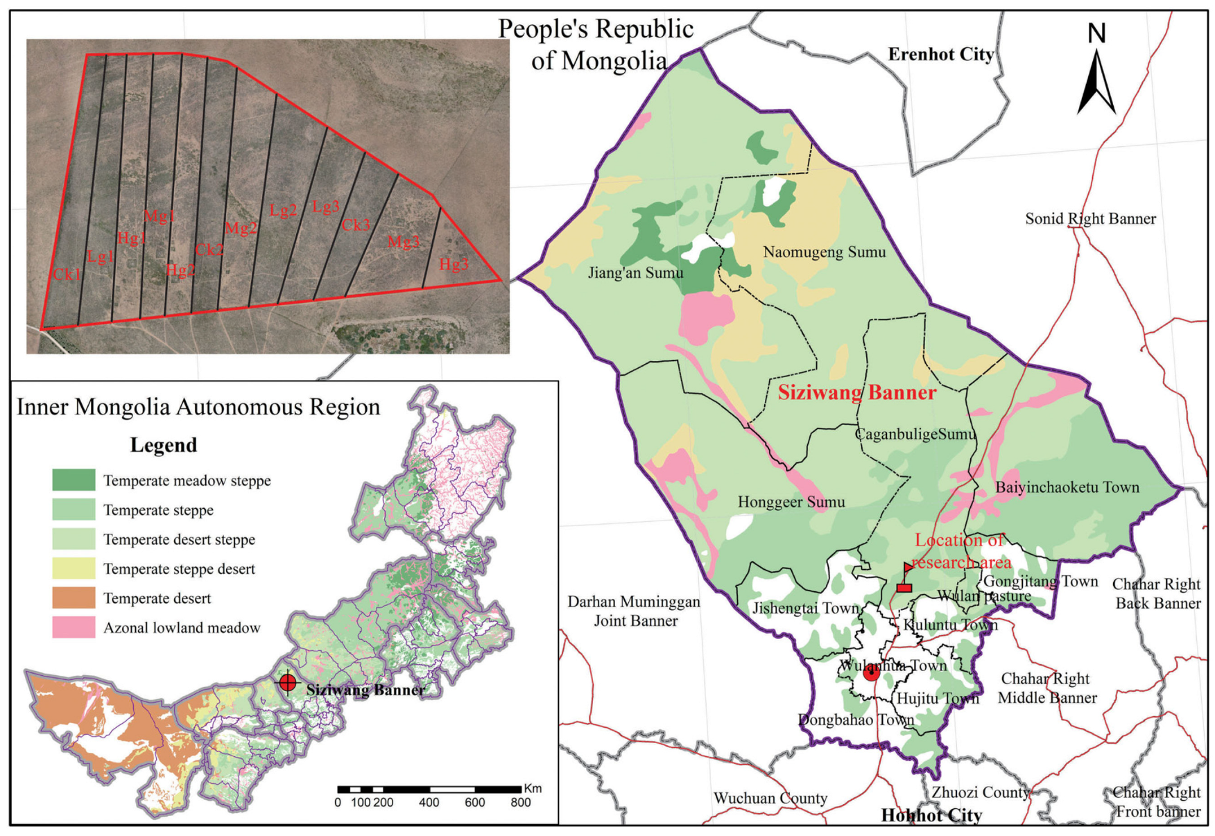
2.1. Study Site Description
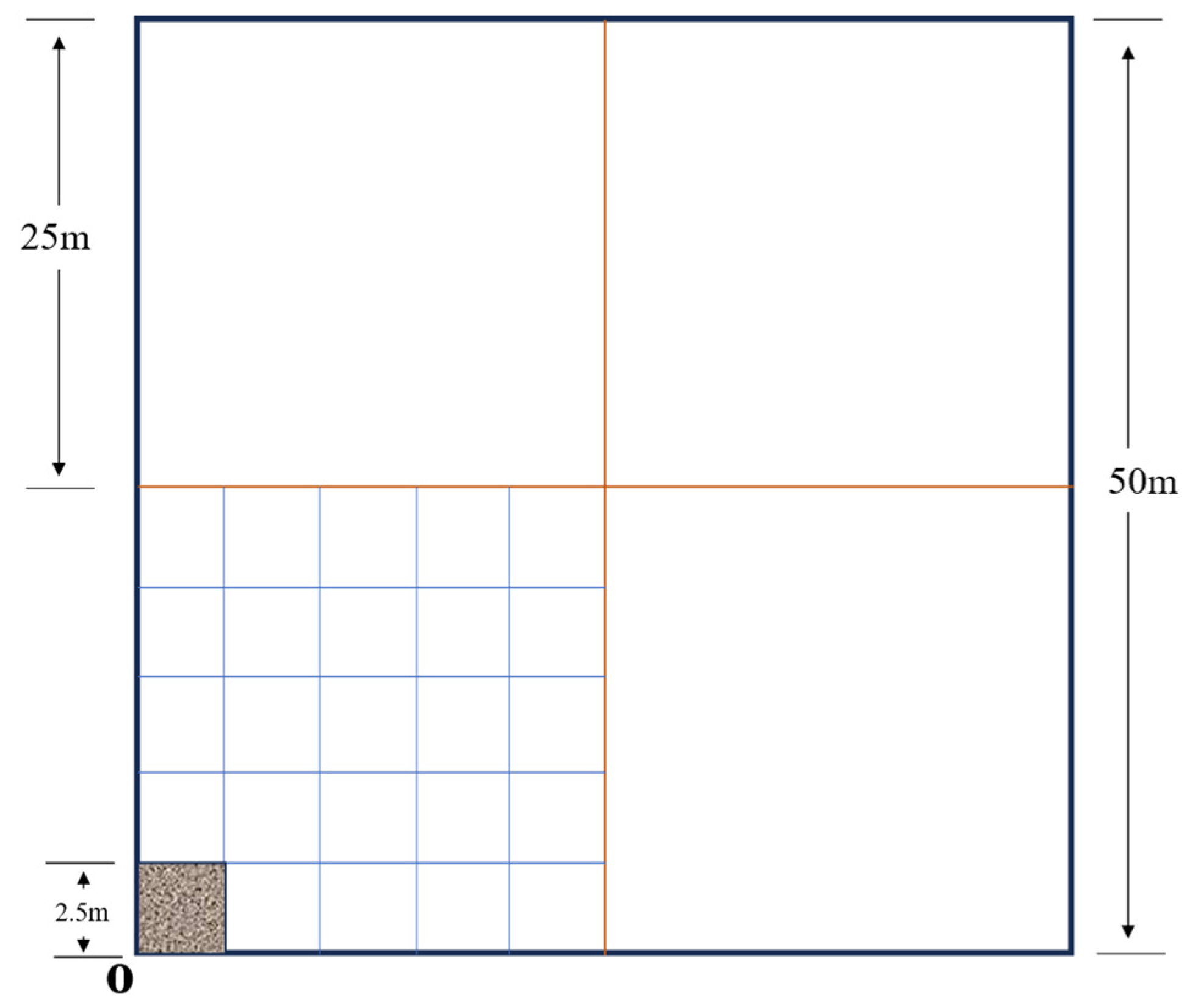
Experimental Setup
2.2. Data Analysis
2.2.1. The Importance Value
2.2.2. The Overall Association
2.2.3. Interspecific Association
2.2.4. Community Stability Index
3. Results
3.1. The Important Value of Species
3.2. The Overall Association of Desert Grasslands
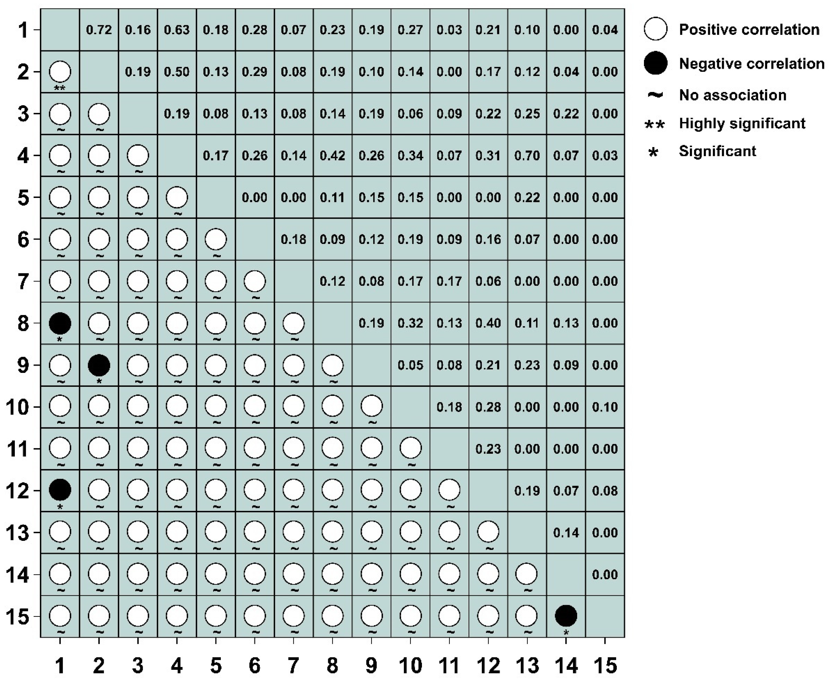
3.3. Test and Comparison of Jaccard Index
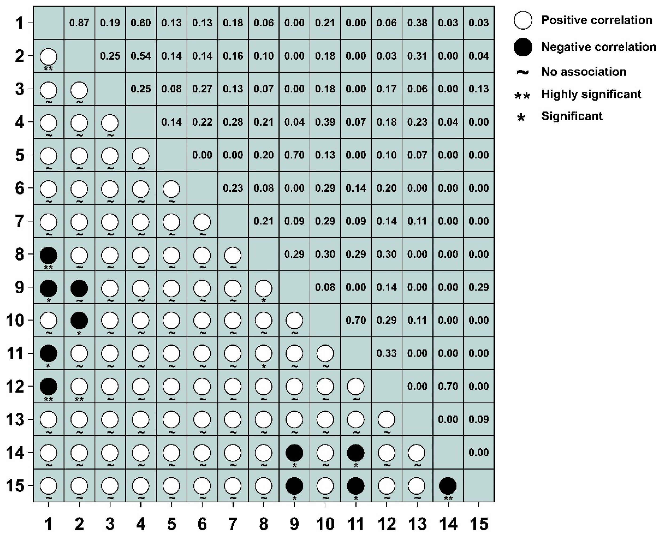
3.4. Test and Jaccard Index Semi-Matrix at Different Spatial Scales
3.4.1. Test and Jaccard Index of 2.5 m × 2.5 m Spatial Scales
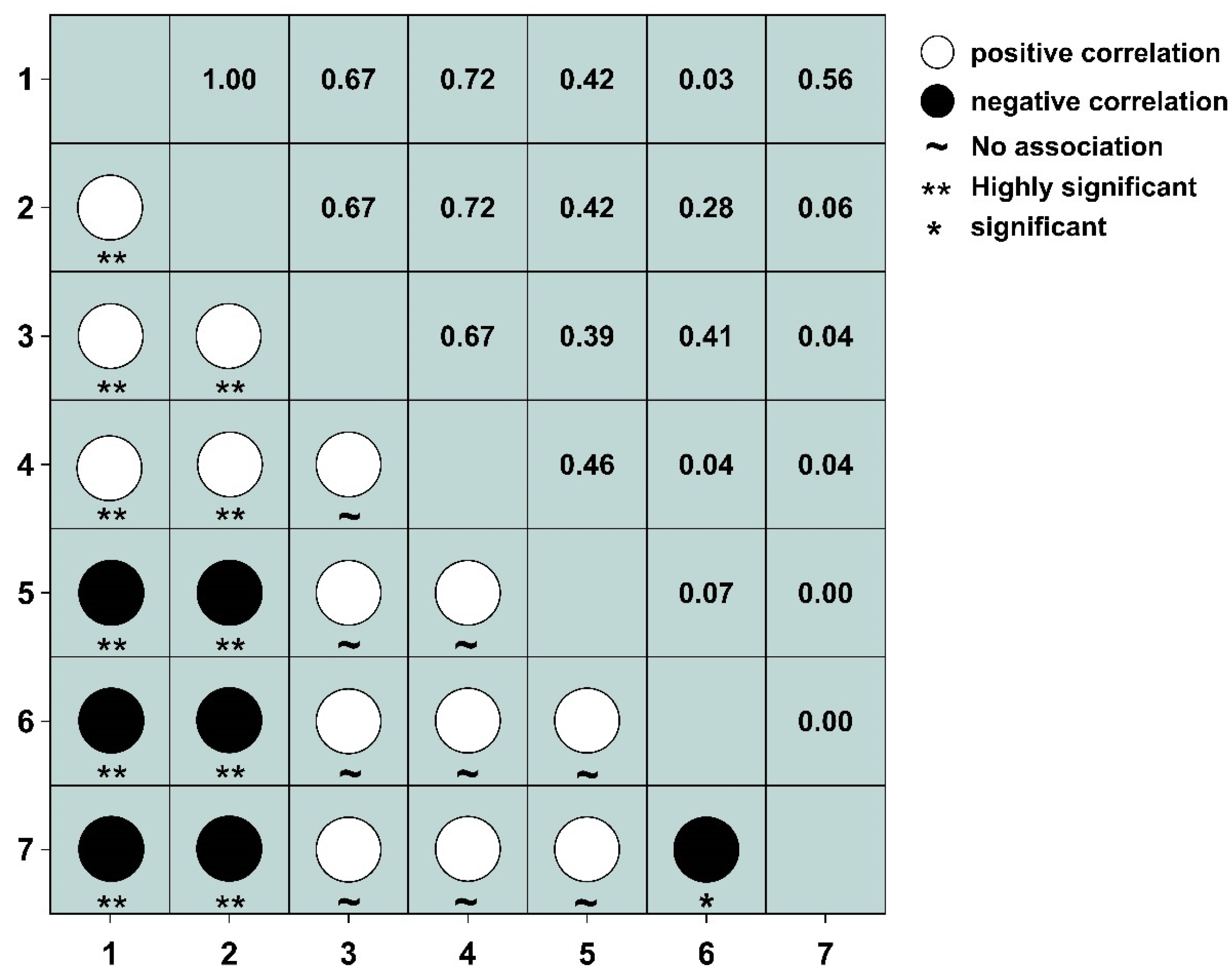
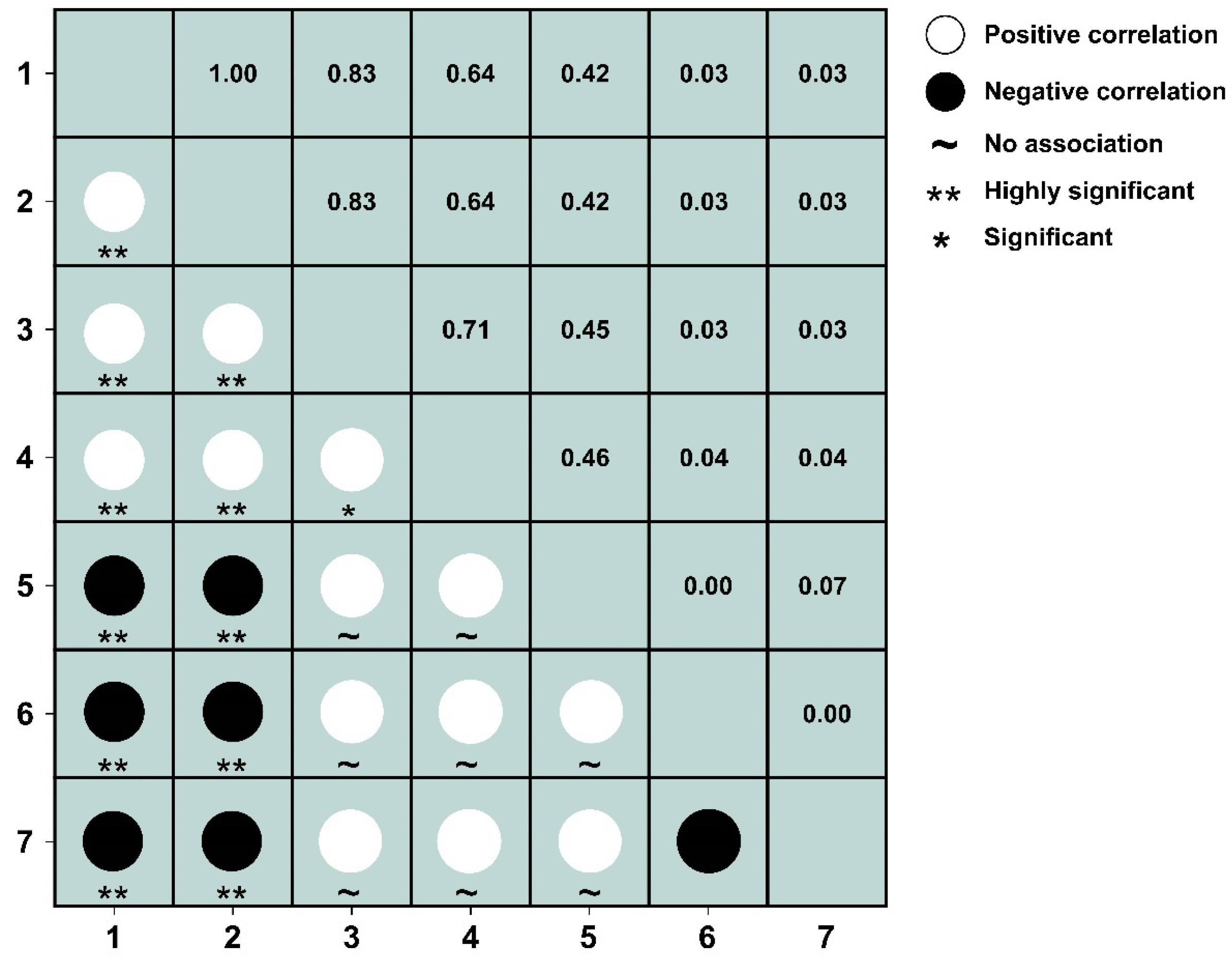
3.4.2. Test and Jaccard Index of 25 m × 25 m Spatial Scales
3.4.3. Test and Jaccard Index of 50 m × 50 m Spatial Scales
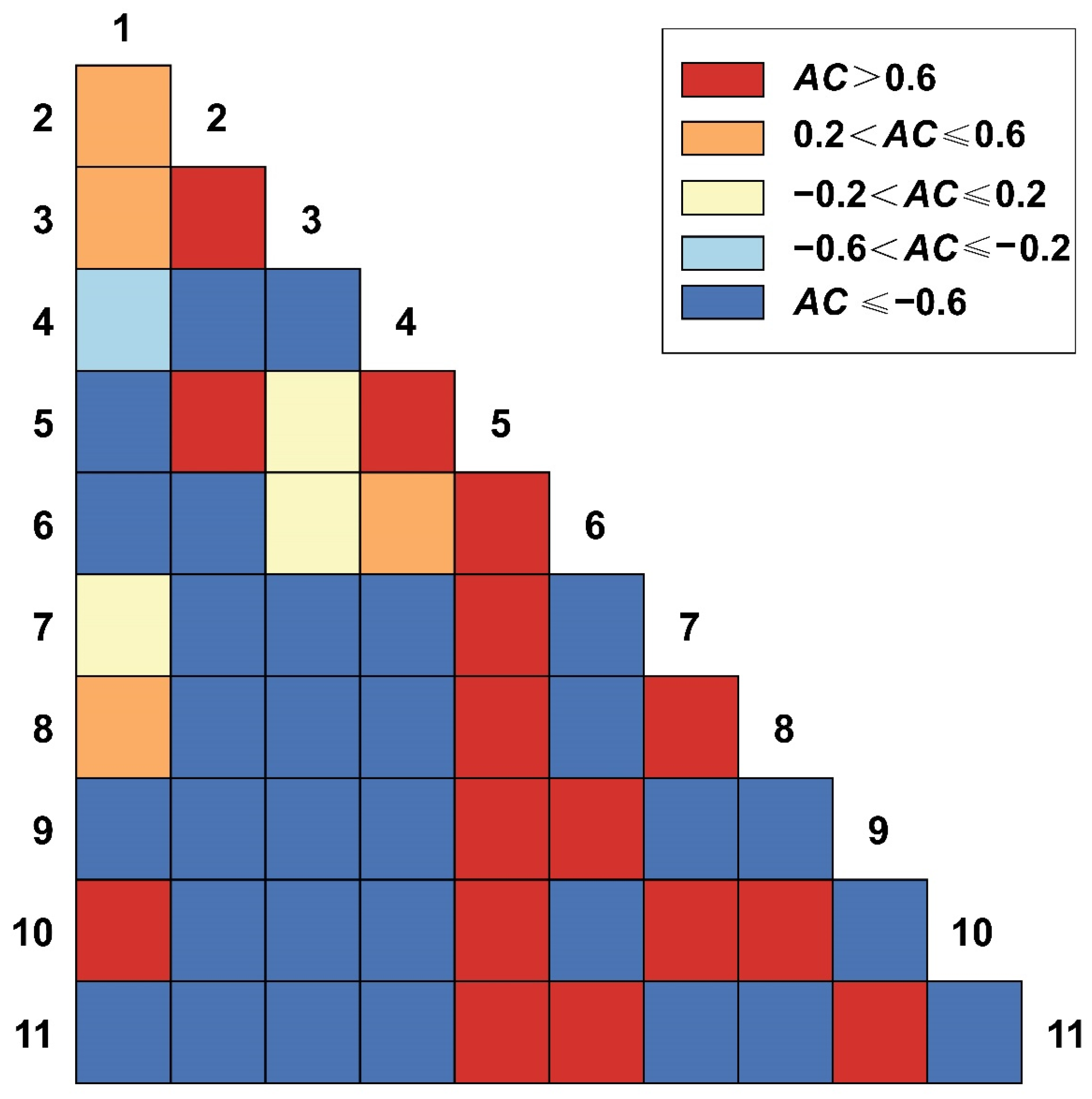
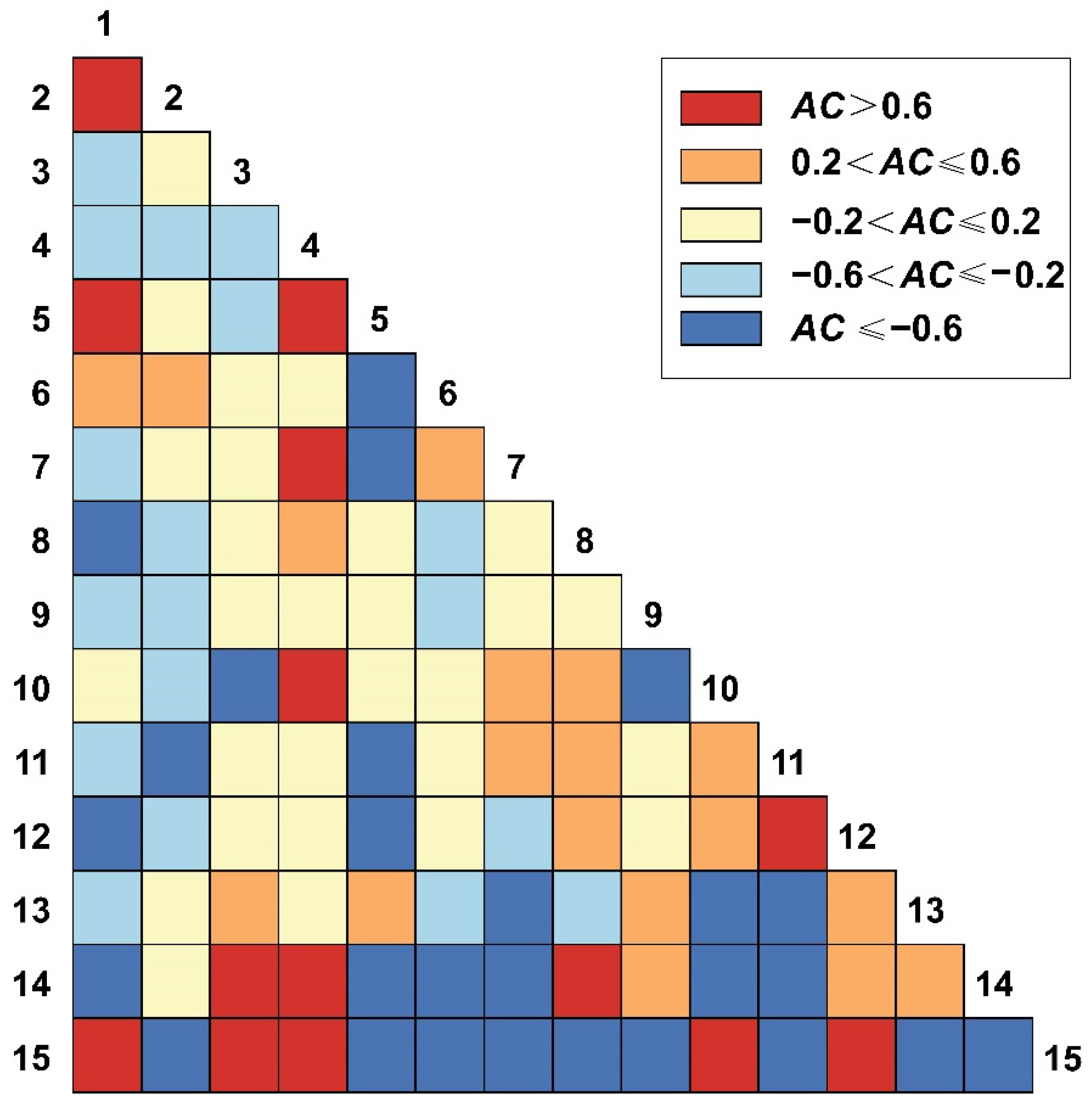
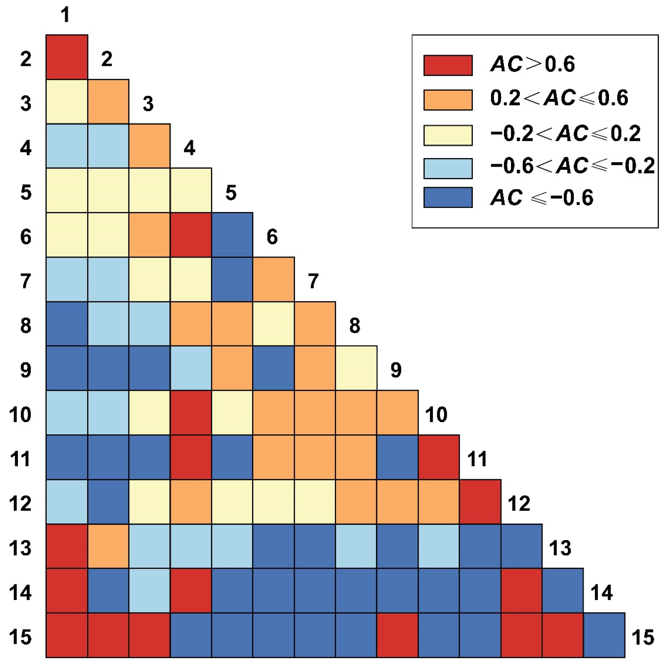
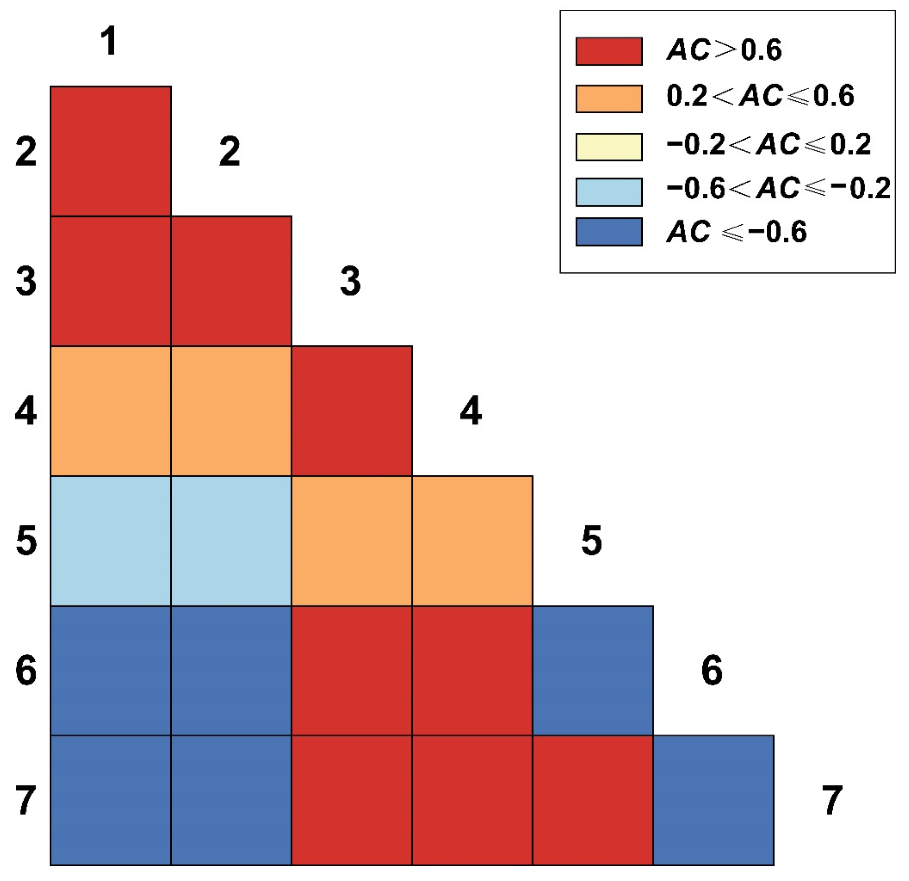
3.5. AC Value Semi-Matrix at Different Spatial Scales
3.5.1. AC Value of 2.5 m × 2.5 m Spatial Scales
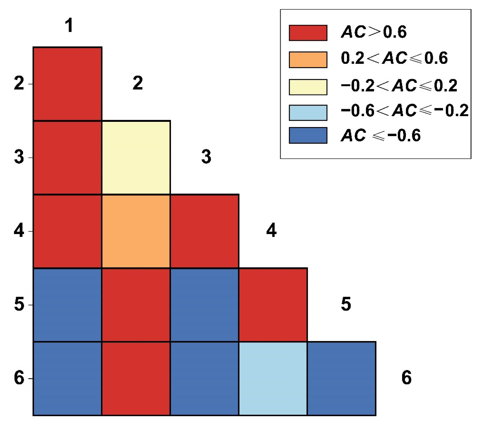
3.5.2. AC Value of 25 m × 25 m Spatial Scales
3.5.3. AC Value of 50 m × 50 m Spatial Scales
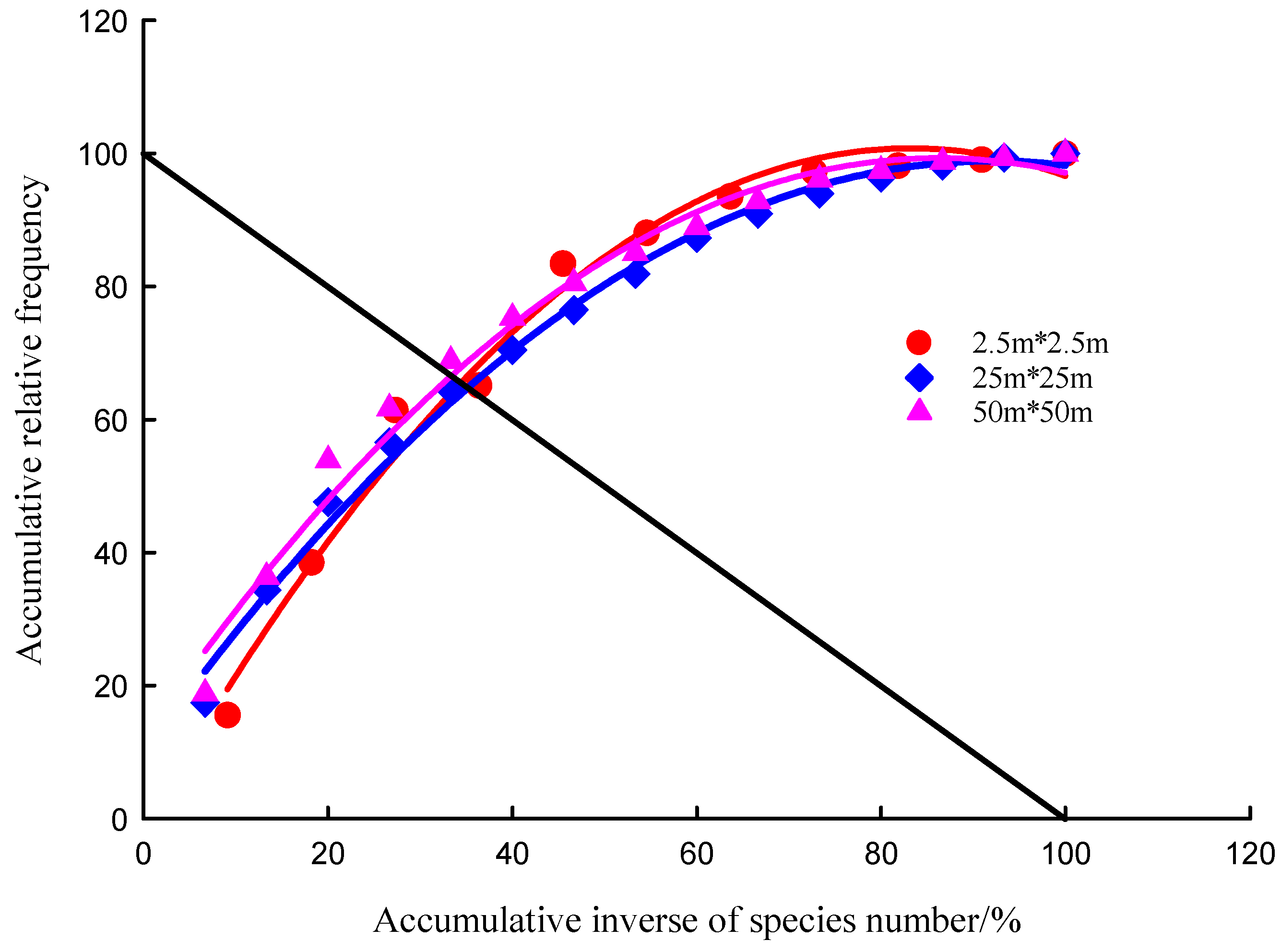
3.6. Plant Community Stability in Desert Steppe
4. Discussion
4.1. Changes in Species Importance Value Under Different Spatial Scales and Grazing Intensity
4.2. Changes in Interspecific Connectivity of Community Species Under Different Spatial Scales and Grazing Intensities
4.3. Changes in Community Stability at Different Spatial Scales and Grazing Intensities
5. Conclusions
Author Contributions
Funding
Institutional Review Board Statement
Informed Consent Statement
Data Availability Statement
Acknowledgments
Conflicts of Interest
References
- Maynard, D.S.; Covey, K.R.; Crowther, T.W.; Sokol, N.W.; Morrison, E.W.; Frey, S.D.; van Diepen, L.T.A.; Bradford, M.A. Species associations overwhelm abiotic conditions to dictate the structure and function of wood-decay fungal communities. Ecology 2018, 99, 801–811. [Google Scholar] [CrossRef] [PubMed]
- Ding, Z.; Ma, K. Identifying changing interspecific associations along gradients at multiple scales using wavelet correlation networks. Ecology 2021, 102, e03360. [Google Scholar] [CrossRef] [PubMed]
- Fridley, J.D.; Lynn, J.S.; Grime, J.P.; Askew, A.P. Longer growing seasons shift grassland vegetation towards more-productive species. Nat. Clim. Chang. 2016, 6, 865–868. [Google Scholar] [CrossRef]
- Gao, W.; Huang, Y.; Lin, J.; Huang, M.; Wu, X.; Lin, W.; Huang, S. Interspecific correlations among dominant populations of natural forest of endangered species Betula fujianensis. Sci. Silvae Sin. 2021, 57, 1–14. [Google Scholar]
- Jin, S.-S.; Zhang, Y.-Y.; Zhou, M.-L.; Dong, X.-M.; Chang, C.-H.; Wang, T.; Yan, D.-F. Interspecific association and community stability of tree species in natural secondary forests at different altitude gradients in the Southern Taihang Mountains. Forests 2022, 13, 373. [Google Scholar] [CrossRef]
- Bronstein, J.L. (Ed.) Mutualism; Oxford Academic: Oxford, UK, 2015. [Google Scholar] [CrossRef]
- Kraft, N.J.; Adler, P.B.; Godoy, O.; James, E.C.; Fuller, S.; Levine, J.M. Community assembly, coexistence and the environmental filtering metaphor. Funct. Ecol. 2015, 29, 592–599. [Google Scholar] [CrossRef]
- Adler, P.B.; Smull, D.; Beard, K.H.; Choi, R.T.; Furniss, T.; Kulmatiski, A.; Meiners, J.M.; Tredennick, A.T.; Veblen, K.E. Competition and coexistence in plant communities: Intraspecific competition is stronger than interspecific competition. Ecol. Lett. 2018, 21, 1319–1329. [Google Scholar] [CrossRef]
- Pausas, J.G.; Verdú, M. The Jungle of Methods for Evaluating Phenotypic and Phylogenetic Structure of Communities. BioScience 2010, 60, 614–625. [Google Scholar] [CrossRef]
- Bronstein, J.L. The evolution of facilitation and mutualism. J. Ecol. 2009, 97, 1160–1170. [Google Scholar] [CrossRef]
- Thackeray, S.J.; Henrys, P.A.; Hemming, D.; Bell, J.R.; Botham, M.S.; Burthe, S.; Helaouët, P.; Johns, D.G.; Jones, I.D.; Leech, D.I.; et al. Phenological sensitivity to climate across taxa and trophic levels. Nature 2016, 535, 241–245. [Google Scholar] [CrossRef]
- Suttie, J.M.; Reynolds, S.G.; Batello, C. (Eds.) Grasslands of the World; Food and Agriculture Organization of the United Nations: Rome, Italy, 2005. [Google Scholar]
- McNaughton, B.L.; O’Keefe, J.; Barnes, C.A. The stereotrode: A new technique for simultaneous isolation of several single units in the central nervous system from multiple unit records. J. Neurosci. Methods 1983, 8, 391–397. [Google Scholar] [CrossRef] [PubMed]
- Battisti, C.; Poeta, G.; Fanelli, G. An Introduction to Disturbance Ecology: A Road Map for Wildlife Management and Conservation. An Introduction to Disturbance Ecology; Springer: Berlin/Heidelberg, Germany, 2016. [Google Scholar]
- Salafsky, N.; Salzer, D.; Stattersfield, A.J.; Hilton-Taylor, C.; Neugarten, R.; Butchart, S.H.; Collen, B.; Cox, N.; Master, L.L.; O’Connor, S.; et al. A standard lexicon for biodiversity conservation: Unified classifications of threats and actions. Conserv. Biol. 2008, 22, 897–911. [Google Scholar] [CrossRef] [PubMed]
- Klein, J.A.; Harte, J.; Zhao, X. Experimental warming causes large and rapid species loss, dampened by simulated grazing, on the Tibetan Plateau. Ecol. Lett. 2004, 7, 1170–1179. [Google Scholar] [CrossRef]
- Sollenberger, L.E.; Vanzant, E.S. Interrelationships among Forage Nutritive Value and Quantity and Individual Animal Performance. Crop. Sci. 2011, 51, 420–432. [Google Scholar] [CrossRef]
- Deng, L.; Sweeney, S.; Shangguan, Z. Grassland responses to grazing disturbance: Plant diversity changes with grazing intensity in a desert steppe. Grass Forage Sci. 2014, 69, 524–533. [Google Scholar] [CrossRef]
- Holechek, J.L.; Pieper, R.D.; Herbel, C.H. Relationship between cattle gain and selected range-site characteristics on shortgrass plains. J. Range Manag. 1982, 35, 309–313. [Google Scholar] [CrossRef]
- Milchunas, D.G.; Lauenroth, W.K.; Chapman, P.L.; Kazempour, M.K. Effects of grazing, topography, and precipitation on the structure of a semiarid grassland. Plant Ecol. 1988, 74, 23–33. [Google Scholar] [CrossRef]
- Derner, J.D.; Boutton, T.W.; Briske, D.D. Grazing and ecosystem carbon storage in the North American Great Plains. Plant Soil 2009, 322, 5–14. [Google Scholar] [CrossRef]
- Brown, J.H.; Kodric-Brown, A. Turnover rates in insular biogeography: Effect of immigration on extinction. Ecology 1977, 58, 445–449. [Google Scholar] [CrossRef]
- Tilman, D. Resource Competition and Community Structure; Princeton University Press: Princeton University Press, 1982. [Google Scholar]
- Gaston, K.J.; Blackburn, T.M. Pattern and Process in Macroecology; Blackwell Science: Hoboken, NJ, USA, 2000. [Google Scholar]
- Jeddi, K.; Chaieb, M. Changes in soil properties and vegetation following livestock grazing exclusion in degraded arid environments of South Tunisia. Flora-Morphol. Distrib. Funct. Ecol. Plants, 2010; 205, 184–189. [Google Scholar]
- Yu, L.; Guo, T.D.; Sun, Z.C.; Ma, Y.P.; Li, Z.L.; Zhao, Y.N.; Wang, H.M. The seed germination characteristics and thresholds of two dominant plants in desertgrassland-shrubland transition of the easten China. Acta Ecol. Sincia 2021, 41, 1–10. [Google Scholar]
- Wang, F.; Pan, X.; Wang, D.; Shen, C.; Lu, Q. Combating desertification in China: Past, present and future. Land Use Policy 2013, 31, 311–313. [Google Scholar] [CrossRef]
- Liu, R.G.; Wang, M.Z.; Guo, S.J.; Liu, L.; Li, X.S. The basic situation of grassland resources in Inner Mongolia Autonomous Region. Grassl. Prataculture 2012, 24, 2–6. [Google Scholar]
- Li, B. The rangeland degradation in north China and its preventive strategy. Sci. Agric. Sin. 1997, 30, 1–10. [Google Scholar]
- Zhang, B.H.; Qu, Z.Q.; Lv, S.J.; Han, G.D.; Gao, C.P.; Wilkes, A.; Li, J.; Li, Z.; Wang, S.; Wang, R.; et al. Grazing effects on total carbon and nitrogen content of wind-eroded soils in desert steppe. Land Degrad. Dev. 2023, 34, 5328–5342. [Google Scholar] [CrossRef]
- Chai, Z.; Sun, C.; Wang, D.; Liu, W. Interspecific associations of dominant tree populations in a virgin old-growth oak forest in the Qinling Mountains, China. Bot. Stud. 2016, 57, 23. [Google Scholar] [CrossRef]
- Feroz, S.M.; Yoshimura, K.; Hagihara, A. Stand stratification and woody species diversity of a subtropical forest in limestone habitat in the northern part of Okinawa Island. J. Plant Res. 2008, 121, 329–337. [Google Scholar] [CrossRef]
- Dolph, S.A. A variance test for detecting species associations, with some example applications. Ecology 1984, 65, 998–1005. [Google Scholar] [CrossRef]
- Zhang, J.T. Quantitative Ecology; Science Press: Beijing, China, 2004. [Google Scholar]
- Li, Y.D.; Xu, H.; Chen, D.; Luo, T.; Mo, J.; Luo, W.; Chen, H.; Jiang, Z. Division of ecological species groups and functional groups based on interspecific association—A case study of the tree layer in the tropical lowland rainforest of Jianfenling in Hainan Island, China. Front. For. China 2008, 4, 407–415. [Google Scholar] [CrossRef]
- Cárdenas, R.E.; Valencia, R.; Kraft, N.J.B.; Argoti, A.; Dangles, O. Plant traits predict inter- and intraspecific variation in susceptibility to herbivory in a hyperdiverse Neotropical rain forest tree community. J. Ecol. 2014, 102, 939–952. [Google Scholar] [CrossRef]
- Lei, S.-L.; Liao, L.-R.; Wang, J.; Zhang, L.; Ye, Z.-C.; Liu, G.-B.; Zhang, C. The diversity–stability relationship of alpine grassland and its environmental drivers. Acta Prataculturae Sin. 2023, 32, 1–12. [Google Scholar]
- Maulidiyan, D.; Ariansyah, E.N.; Zubaidah, S.; Widiastuti, E.; Bekti, H.S.; Larasati, A.D.; Sari, R.; Trijunianto, A.; Aziz, S.; Diany, E.; et al. Vegetation structure and composition on Rafflesia zollingeriana habitat in Meru Betiri National Park. IOP Conf. Ser. Earth Environ. Sci. 2019, 394, 012010. [Google Scholar] [CrossRef]
- Perronne, R.; Munoz, F.; Borgy, B.; Reboud, X.; Gaba, S. How to design trait-based analyses of community assembly mechanisms: Insights and guidelines from a literature review. Perspect. Plant Ecol. Evol. Syst. 2017, 25, 29–44. [Google Scholar] [CrossRef]
- Yan, R.R.; Xin, X.P.; Yan, Y.; Wang, X.; Zhang, B.; Yang, G.; Liu, S.; Deng, Y.; Li, L. Impacts of differing grazing rates on canopy structure and species composition in Hulunber meadow steppe. Rangel. Ecol. Manag. 2015, 68, 54–64. [Google Scholar] [CrossRef]
- Chase, J.M.; Leibold, M.A. Ecological Niches: Linking classical and contemporary approaches to niche theory. Ecol. Lett. 2003, 6, 667–679. [Google Scholar]
- Huston, M.A. Local processes and regional patterns: Appropriate scales for understanding variation in the diversity of plants and animals. Oikos 1999, 86, 393–401. [Google Scholar] [CrossRef]
- Pastore, A.I.; Barabás, G.; Bimler, M.D.; Mayfield, M.M.; Miller, T.E. The evolution of niche overlap and competitive differences. Nat. Ecol. Evol. 2021, 5, 330–337. [Google Scholar] [CrossRef]
- Liu, Z.; Chang, Q.; Gao, J. Impact of grazing intensity on plant community diversity and composition in alpine grasslands in the Qinghai–Tibet Plateau. Land Degrad. Dev. 2019, 30, 21–33. [Google Scholar]
- Macarthur, R.H.; Levins, R.A. The Limiting Similarity, Convergence, and Divergence of Coexisting Species. Am. Nat. 1967, 101, 377–385. [Google Scholar] [CrossRef]
- Li, H.-D.; Wu, X.-W.; Xiao, Z.-S. Assembly, ecosystem functions, and stability in species interaction networks. Chin. J. Plant Ecol. 2021, 45, 1049–1063. [Google Scholar] [CrossRef]
- Lv, G.Y.; Wang, Z.Y.; Guo, N.; Xu, X.B.; Liu, P.P.; Wang, C.J. Status of Stipa breviflora as the constructive species will be lost under climate change in the temperate desert steppe in the future. Ecol. Indic. 2021, 126, 107715. [Google Scholar] [CrossRef]
- Zhou, S.X.; Peng, Y.S.; Ding, J.M.; Gao, P.X.; Li, G.L.; Wang, M.; Lv, F. Analysis of community stability and inter-specific correlations among dominant woody populations of the endangered plant Sinojackia rehderiana communities. Guihaia 2017, 37, 442–448. [Google Scholar]
- Wu, Q.; Ren, H.Y.; Wang, Z.W.; Li, Z.G.; Liu, Y.H.; Wang, Z.; Li, Y.; Zhang, R.; Zhao, M.; Chang, S.X.; et al. Additive negative effects of decadal warming and nitrogen addition on grassland community stability. J. Ecol. 2020, 108, 1442–1452. [Google Scholar] [CrossRef]


| No. | Species | Important Value IV | |||||
|---|---|---|---|---|---|---|---|
| 2.5 m × 2.5 m | 25 m × 25 m | 50 m × 50 m | |||||
| No Grazing | Heavy Grazing | No Grazing | Heavy Grazing | No Grazing | Heavy Grazing | ||
| 1 | Stipa breviflora | 0.42 | 0.52 | 0.3 | 0.41 | 0.35 | 0.36 |
| 2 | Cleistogenes songorica | 0.21 | 0.1 | 0.11 | 0.15 | 0.18 | 0.18 |
| 3 | Caragana stenophylla | 0.16 | 0.04 | 0.00 | 0.04 | ||
| 4 | Asparagus | 0.01 | 0.00 | 0.00 | |||
| 5 | Convolvulus ammannii | 0.12 | 0.00 | 0.17 | 0.03 | 0.16 | 0.04 |
| 6 | Lagochilus ilicifolium | 0.03 | 0.01 | 0.01 | |||
| 7 | Allium tenuissimum | 0.01 | 0.03 | 0.02 | |||
| 8 | Krascheninnikovia ceratoides | 0.01 | 0.1 | 0.06 | |||
| 9 | Kochia prista | 0.00 | 0.05 | 0.02 | |||
| 10 | Leymus chinensis | 0.03 | 0.02 | 0.00 | |||
| 11 | Artemisia frigida | 0.06 | 0.05 | ||||
| 12 | Potentilla bifurca | 0.01 | 0.00 | 0.01 | |||
| 13 | Chenopodidm glaucum | 0.02 | 0.02 | ||||
| 14 | Chenopodium aristatum | 0.01 | 0.3 | 0.02 | 0.33 | 0.04 | 0.36 |
| 15 | Cleistogenes squarrosa | 0.00 | |||||
| 16 | Salsola collina | 0.00 | 0.01 | 0.04 | 0.01 | 0.00 | |
| 17 | Parthenocissus tricuspidata | 0.06 | 0.06 | 0.05 | |||
| 18 | Stipa krylovii | 0.01 | |||||
| 19 | Neopalasia spectate | 0.00 | |||||
| Spatial Scale | Habitat Type | Variance Ratio | Statistic W | (Chi0.95, Chi0.05) | Association |
|---|---|---|---|---|---|
| 2.5 m × 2.5 m | No grazing | 1.03 | 25.67 | (14.61, 37.65) | Positive correlation, not significant |
| Heavy grazing | 1.24 | 30.91 | (14.61, 37.65) | Positive correlation, not significant | |
| 25 m × 25 m | No grazing | 0.65 | 23.41 | (23.27, 51.00) | Negative correlation, not significant |
| Heavy grazing | 1.26 | 45.46 | (23.27, 51.00) | Positive correlation, not significant | |
| 50 m × 50 m | No grazing | 0.69 | 24.96 | (23.27, 51.00) | Negative correlation, not significant |
| Heavy grazing | 1.67 | 59.83 | (23.27, 51.00) | Positive correlation, significant |
| . | Jaccard Index | ||||||||
|---|---|---|---|---|---|---|---|---|---|
| Spatial Scales | Habitat Type | Pair Species Number | Positive Association | No Association | Negative Association | Positive and Negative Association Ratio | JI ≥ 0.3 | JI < 0.3 | JI = 0 |
| 2.5 m × 2.5 m | No grazing | 55 | 8 (14.55%) | 31 (56.36%) | 16 (29.09%) | 0.5 | 9 (16.36%) | 46 (83.64%) | 17 (30.91%) |
| Heavy grazing | 15 | 5 (33.33%) | 6 (40%) | 4 (26.67%) | 1.25 | 6 (40%) | 9 (60%) | 1 (6.67%) | |
| 25 m × 25 m | No grazing | 105 | 1 (0.95%) | 100 (95.24%) | 4 (3.81%) | 0.25 | 9 (8.57%) | 96 (91.43%) | 24 (22.83%) |
| Heavy grazing | 21 | 5 (23.81%) | 9 (42.86%) | 7 (33.33%) | 0.71 | 12 (57.14%) | 9 (42.86%) | 2 (9.52%) | |
| 50 m × 50 m | No grazing | 105 | 4 (3.81%) | 91 (86.67%) | 10 (9.52%) | 0.4 | 11 (10.48%) | 94 (89.52%) | 35 (33.33%) |
| Heavy grazing | 21 | 6 (28.57%) | 8 (38.1%) | 7 (33.33%) | 0.86 | 10 (47.62%) | 11 (52.38%) | 2 (9.52%) | |
| Spatial Scale | Habitat Type | Fitting Equation | Determination Coefficient | Intersection Coordinate | Euclidean Distance | Stability |
|---|---|---|---|---|---|---|
| 2.5 m × 2.5 m | No grazing | 0.9875 | (34.44, 65.56) | 20.42 | unstable | |
| Heavy grazing | 0.9868 | (38.51, 61.49) | 26.17 | unstable | ||
| 25 m × 25 m | No grazing | 0.9941 | (35.16, 64.84) | 21.44 | unstable | |
| Heavy grazing | 0.9985 | (36.63, 63.37) | 23.52 | unstable | ||
| 50 m × 50 m | No grazing | 0.9858 | (33.39, 66.61) | 18.94 | unstable | |
| Heavy grazing | 0.9986 | (36.42, 63.58) | 23.22 | unstable |
Disclaimer/Publisher’s Note: The statements, opinions and data contained in all publications are solely those of the individual author(s) and contributor(s) and not of MDPI and/or the editor(s). MDPI and/or the editor(s) disclaim responsibility for any injury to people or property resulting from any ideas, methods, instructions or products referred to in the content. |
© 2024 by the authors. Licensee MDPI, Basel, Switzerland. This article is an open access article distributed under the terms and conditions of the Creative Commons Attribution (CC BY) license (https://creativecommons.org/licenses/by/4.0/).
Share and Cite
Du, X.; Zhang, J.; Liu, J.; Lv, S.; Liu, H. Effects of Heavy Grazing on Interspecific Relationships at Different Spatial Scales in Desert Steppe of China. Sustainability 2024, 16, 10059. https://doi.org/10.3390/su162210059
Du X, Zhang J, Liu J, Lv S, Liu H. Effects of Heavy Grazing on Interspecific Relationships at Different Spatial Scales in Desert Steppe of China. Sustainability. 2024; 16(22):10059. https://doi.org/10.3390/su162210059
Chicago/Turabian StyleDu, Xiaoyu, Jun Zhang, Juhong Liu, Shijie Lv, and Haijun Liu. 2024. "Effects of Heavy Grazing on Interspecific Relationships at Different Spatial Scales in Desert Steppe of China" Sustainability 16, no. 22: 10059. https://doi.org/10.3390/su162210059
APA StyleDu, X., Zhang, J., Liu, J., Lv, S., & Liu, H. (2024). Effects of Heavy Grazing on Interspecific Relationships at Different Spatial Scales in Desert Steppe of China. Sustainability, 16(22), 10059. https://doi.org/10.3390/su162210059