Development of Particulate Matter Concentration Estimation Models for Road Sections Based on Micro-Data

Abstract

With increasing global concerns related to global warming, air pollution, and environmental health, South Korea is actively implementing various particulate matter (PM) reduction policies to improve air quality. Accurate data analysis, including the investigation of weather phenomena, monitoring, and integrated prediction, is essential for effective PM reduction. However, the factors influencing the PM generated from domestic road sections have not yet been systematically analyzed, and currently, no predictive models utilize weather and traffic data. This study analyzed the correlations among factors influencing PM to develop models for estimating fine and coarse PM (PM_2.5 and PM₁₀, respectively) concentrations in road sections. Regression analysis models were used to assess the sensitivity of PM_2.5 and PM₁₀ concentrations to the traffic volume, whereas machine learning-based models, including linear regression, convolutional neural networks, and random forest models, were constructed and compared. The random forest models outperformed the other models, with coefficients of determination of 0.74 and 0.71 and mean absolute errors of 5.78 and 9.60 for PM_2.5 and PM₁₀, respectively. These results indicate that the random forest model provides the most accurate PM concentration estimates for road sections. The practical applications of the developed models were considered to inform effective transportation policies aimed at reducing PM. The developed model has practical applications in the formulation of transportation policies aimed at reducing PM. In particular, the model will play an important role in data-driven policymaking for sustainable urban development and environmental protection. By analyzing the correlation between traffic volume and weather conditions, policymakers can formulate more effective and sustainable strategies for reducing air pollution.

1. Introduction

Since particulate matter (PM) was classified as a “class one carcinogen” by the World Health Organization (WHO) in 2013, the awareness of PM levels in the atmosphere has increased worldwide [1]. As various pollutants, such as PM, and greenhouse gasses continue to affect human health and threaten the global environment, efforts are being made worldwide to reduce the release of PM into the environment. The transportation sector is a primary source of fine and coarse PM (PM_2.5 and PM₁₀, respectively). Accordingly, related government ministries and research institutes are investigating strategies for reducing the PM generated by the transportation sector.

In Korea, no models currently exist for the atmospheric diffusion of PM around roads. Some Korean researchers have estimated the concentrations of PM from road traffic pollutants in surrounding areas by using models developed specifically for conditions in the United States (e.g., Lee and Hahn [2]; Yang et al. [3]). Atmospheric diffusion models, such as the American Meteorological Society/Environmental Protection Agency Regulatory Model (AERMOD), require precise weather data. However, applying such complex models in Korea is challenging owing to the lack of a lead institution that constructs and manages the input data. Moreover, the US models have not been calibrated for application in Korea; therefore, the estimated PM values from US-based models are likely to be inaccurate.

This study develops and evaluates highly reliable, domestically suitable, and easy-to-analyze models for estimating PM_2.5 and PM₁₀ concentrations in Korea. Specifically, this study correlates traffic and weather phenomena with PM concentrations in areas close to roads and constructs models capable of determining PM concentrations in road sections. Therefore, different road sections can be classified according to their characteristics. The traffic volume, weather conditions (e.g., temperature, humidity, and precipitation), background concentration, and PM_2.5 and PM₁₀ concentrations for road sections in Korea were collected and used to construct data, based on which the correlations among the traffic and weather conditions for the road sections were established. Then, the sensitivity of PM concentrations to the traffic volume was analyzed using statistical models. PM concentration estimation models for road sections were developed through machine learning. Finally, the transferability of the models was verified to validate their reliability.

The model developed in this study may be used to analyze the correlation between traffic volume and weather conditions to suggest effective air pollution management strategies. This will provide essential data for policymakers to formulate transportation and environmental policies, contributing to the realization of sustainable transportation systems.

2. Literature Review

Various factors significantly affect pollutant concentrations in areas close to roads. Jacob and Winner [4] correlated weather factors with air quality, considering weather conditions measured by weather stations, and their analysis was mainly based on temperature, precipitation, relative humidity, and wind speed data. The study revealed a consistent and positive correlation between PM and regional stagnation and between PM and humidity (

Table 1. Correlations between weather factors and air quality.

Variable	PM
Temperature	−
Wind speed	−
Atmospheric mixing height	−−
Humidity	+
Cloud cover	−
Precipitation	−−

Note: + positive correlation, − negative correlation, −− consistent negative correlation [4].

). It revealed that PM is consistently and negatively correlated with the atmospheric mixing height and precipitation and is negatively correlated with temperature, wind speed, and cloud cover.

Zhang et al. [5] reported that pollutant concentrations in areas close to roads may increase simultaneously with the total amount of road pollutants. They suggested that traffic variables such as the traffic volume, travel speed, and vehicle composition should be considered when estimating pollutant concentrations in areas close to roads because traffic characteristics affect the amount of road pollutants generated.

Wu and Niemeier [6] reported that pollutant concentrations decrease with increasing distance from a road segment. The Health Effects Institute (Boston, MA, USA) [7] estimated the sphere of influence of road pollutants to be <200 m, suggesting that pollutant concentrations increase toward roads and reach background concentration levels when the distance exceeds 200 m.

Tecer et al. [8] reported that pollutant concentrations are significantly affected by various weather conditions (e.g., temperature, humidity, wind direction, and wind speed) and that wind speed is a crucial weather factor. Generally, pollutant concentrations in areas close to roads decrease with increasing wind speed because pollutants spread more rapidly in the atmosphere. In addition, surface temperature and precipitation reduce pollutant concentrations in areas near roads. In contrast, Lin et al. [9] suggested that humidity, pressure, and cloud cover negatively correlate with pollutant concentrations. In other words, pollutant concentrations in areas close to roads may increase as humidity increases.

Table 2. Correlations between road traffic pollutant concentrations and influencing factors.

Variable	Correlation	Source
Pollutant emissions	+	[10,11]
Distance from emission source	−	[6,12,13]
Wind speed	−	[5,8,12,14]
Surface temperature	−	[5,8,10,14]
Precipitation	−	[8,10]
Humidity	+	[5,8,14,15]
Pressure	+	[14]
Cloud cover	+	[8]
Heat island effect	+/−	[16]

Note: “+” represents a positive correlation between pollutant concentrations and the influencing factor; “−” indicates a negative correlation [17].

summarizes the correlations established in previous studies between road and weather conditions (influencing factors) and pollutant concentrations.

By analyzing 11 years of observation data across the United States, Tai et al. [18] investigated the correlations between PM_2.5 concentrations and weather variables. They constructed a multiple linear regression model using weather variables (e.g., temperature, humidity, precipitation, circulation, and cloud cover) and concluded that approximately 50% of the daily fluctuations in PM_2.5 concentrations can be controlled. They also reported that PM_2.5 concentrations can increase by 2.6 μm/m³ on average under atmospheric stagnation.

Kim et al. [17] suggested that improving the efficiency of the regional-scale analysis of road air quality is important for assessing the impacts of traffic control policies for regional PM reduction. Therefore, they used machine learning models and the random forest algorithm to effectively predict air quality. To characterize the spread of road pollutants, they selected links with direct influence and used screening models to select road sections. They used six variables, including urban variables and weather conditions, and secured a 97% or higher prediction rate depending on the road network, section, weather, and PM concentrations. However, this involves macroscopic analysis, and applying a practical PM concentration diffusion model for areas close to roads is difficult.

Askariyeh et al. [19] conducted a pairwise comparison between the observed PM concentrations around highways (individually collected monitoring data) and the National Ambient Air Quality Standard. The comparison revealed a high correlation between the background concentrations and the concentrations around roads. The regression analysis of PM_2.5 around roads and monitoring data revealed an increase of approximately 23% compared with the background concentration data [11].

For PM concentrations, wind speed, and wind direction, three key accuracy metrics (Pearson’s correlation coefficient, coefficient of determination, and root mean squared error (RMSE)) revealed that multiple linear regression models performed better than linear regression models that used the background concentration as the only predictive variable. The modified R² obtained for the multiple linear regression model revealed that 83% of the variability in 24 h PM_2.5 concentrations on surrounding roads can be explained as a function of background PM_2.5 concentrations, wind speed, and wind direction.

The literature review revealed that various factors affect pollutant concentrations in areas close to roads. In other words, various influencing factors must be considered when constructing a model for predicting pollutant concentrations in areas close to roads. In this study, various factors presented in the literature were considered analysis variables, and final models were constructed considering the feasibility of collecting actual data.

Research on roadside PM concentration estimation considering domestic environmental conditions is lacking. This study implemented the following key points:

• PM concentrations around roads could not be measured because of the absence of PM sensor installation points; thus, PM data around roads not considered in previous studies were applied.
• When factors affecting PM were considered, accurate correlations were challenging to identify because the regional traffic volume data were variable. This study, however, is differentiated by applying directly related traffic volume data.
• Previous studies collected short-term data, and climate change could not be reflected owing to limitations, such as survey costs and regional characteristics. However, in this study, data were collected over a long period, approximately six months, which included summer, autumn, and winter months.

3. Data Collection and Analysis

3.1. Data Collection at Monitoring Points

Two traffic volume monitoring points operated by the Korea Institute of Civil Engineering and Building Technology (KICT) were selected for traffic volume, temperature, and humidity data collection.

Table 3. Locations of the monitoring points.

Monitoring Point	Route	Address
Point 1	National road 38	1065-6, Wonjeong-ri, Poseung-eup, Pyongtaek-si, Gyeonggi-do, Korea (latitude: 37.004214; longitude: 126.829239)
Point 2	National road 34	496-2, Sinbong-ri, Yeongin-myeon, Asan-si, Chungcheongnam-do, Korea (latitude: 36.898071; longitude: 126.984613)

presents the locations of the monitoring points. PM sensors were installed at these monitoring points, and measurement data from the sensors were collected via wireless communication.

Real-time traffic volume data at the monitoring points were collected and stored in the road traffic volume collection server of the KICT. The data comprised vehicle type, individual vehicle, and traffic volume data collected at 5 min intervals. The sensors comprised one loop sensor and two piezo sensors per lane. When a vehicle passed through both sensors, the traffic volume and vehicle type data were collected by the controller and transmitted every 5 min. The road traffic volume survey equipment was more than 95% reliable (highest class), because regular inspections of the equipment were performed.

The PM concentration was measured using a Smart AirRuler AM100 (MAT Inc., Gyeonggi-do, Republic of Korea). This equipment, which is certified as Class 1 (more than 95% reliable) by the Korea Meteorological Administration (KMA), can measure a wide range of PM concentrations (0–1000 μg/m³), making it suitable for PM concentration measurement. The specific data items measured and collected were temperature, humidity, PM_2.5, PM₁₀, date, and time.

3.2. Background Concentration Data Collection

Background concentrations refer to PM concentrations at locations not influenced by the traffic volume or vehicle traffic (i.e., points considerably away from roads). Background concentrations comprise pollutant concentrations formed by pollution sources (i.e., natural environment pollution sources, such as yellow dust, and general urban pollution sources, such as power plants and heating) other than those formed by traffic.

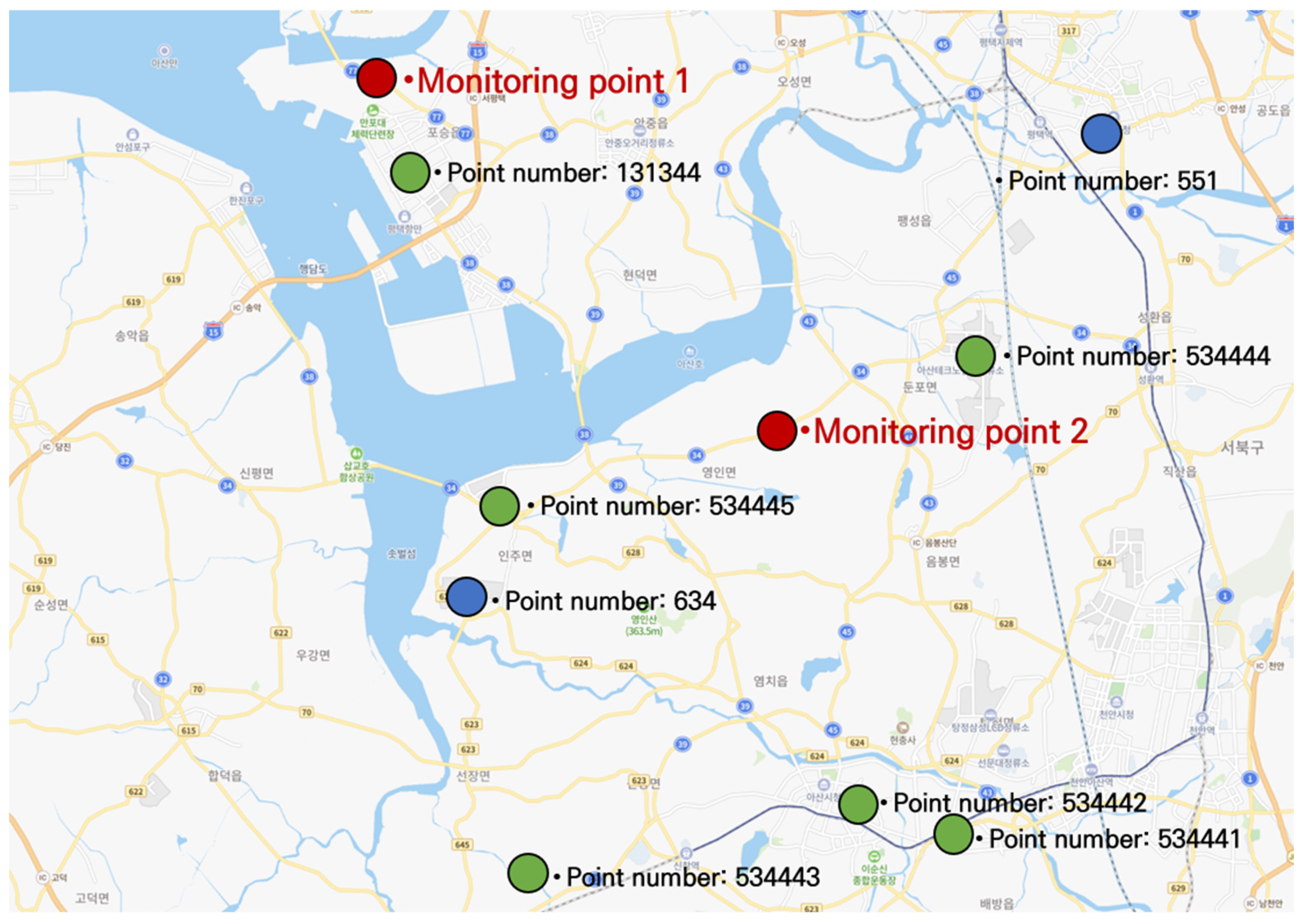
This study utilized hourly PM concentration measurement data collected by Air Korea (airkorea.or.kr). Air Korea—which is operated by the Korea Environment Corporation, an affiliate of the Ministry of Environment—provides air quality information from across the country in real time. The Air Korea measurement points for the background PM concentration for the study area are as follows (Figure 1):

• Point number 534441: 573-2, Mojong-dong, Asan-si, Chungnam;
• Point number 534442: 38, Baebang-ro, Baebang-eup, Asan-si, Chungnam;
• Point number 534443: 296-4, Gigok-ri, Dogo-myeon, Asan-si, Chungnam;
• Point number 534444: 1481, Seokgok-ri, Dunpo-myeon, Asan-si, Chungnam;
• Point number 534445: 23-28, Injusandan-ro, Inju-myeon, Asan-si, Chungnam;
• Point number 131344: 38, Pyeongtaekhang-ro 184beon-gil, Poseung-eup, Pyeongtaek-si, Gyeonggi.

3.3. Weather Data

In this study, weather-related factors (wind direction, wind speed, precipitation, and pressure) were collected through the weather data open portal of the KMA (https://data.kma.go.kr/cmmn/main.do, accessed on 17 May 2021).

The data from two KMA measurement points adjacent to the traffic volume–PM monitoring points were collected. The locations of these points are as follows (Figure 1):

• Point number 551 (latitude: 36.98769; longitude: 127.10879);
• Point number 634 (latitude: 36.84578; longitude: 126.86536).

3.4. Data Construction and Descriptive Statistics

Table 4. Descriptive statistics of data.

Category	Variable		Collection Rate	Minimum Value	Maximum Value	Average	Standard Deviation
Monitoring point	1	Traffic volume (units)	97.6%	1.0	409.0	141.4	94.3
		PM2.5 (μg/m3)	99.1%	0.0	361.0	26.9	21.1
		PM10 (μg/m3)	99.1%	0.0	895.0	45.7	40.9
	2	Traffic volume (units)	97.5%	0.0	322.0	53.2	62.0
		PM2.5 (μg/m3)	98.5%	0.0	159.0	21.4	18.1
		PM10 (μg/m3)	98.5%	0.0	461.0	28.7	28.1
Background concentration	551	Temperature (°C)	99.8%	−11.2	35.2	12.9	11.0
		Humidity (%)	99.8%	20.6	99.9	73.6	19.1
		Wind speed (m/s)	99.8%	0.0	9.5	1.6	1.2
		Precipitation (mm)	99.8%	0.0	33.5	0.2	1.2
	634	Temperature (°C)	100.0%	−10.7	35.2	12.9	10.9
		Humidity (%)	100.0%	22.4	99.9	70.1	19.4
		Wind speed (m/s)	100.0%	0.0	11.1	1.9	1.4
		Precipitation (mm)	100.0%	0.0	23.5	0.1	1.0
Background concentration	PM2.5	Total	94.9%	0.0	161.0	26.9	19.6
		534,441	92.0%	0.0	151.0	27.0	19.8
		534,442	95.5%	0.0	147.0	23.5	17.2
		534,443	95.5%	0.0	122.0	25.7	19.0
		534,444	94.0%	0.0	159.0	31.5	21.9
		534,445	97.5%	0.0	161.0	27.0	19.0
	PM10	Total	97.0%	0.0	235.0	43.5	25.7
		534,441	96.4%	0.0	235.0	41.2	26.4
		534,442	96.4%	3.0	202.0	41.4	20.5
		534,443	98.0%	0.0	230.0	41.0	26.1
		534,444	96.4%	0.0	227.0	47.2	27.8
		534,445	97.8%	0.0	233.0	46.6	26.0

presents the statistical properties of the data collected from various sources. The table reveals that the traffic volume and PM concentration data collected from the installed measuring instruments varied considerably. For example, the traffic volume on the roads varied from 1 to 409 units per 5 min (monitoring point 1) and from 0 to 322 units per 5 min (monitoring point 2).

As shown in Table 4, the PM concentrations around the road fluctuated significantly. The PM_2.5 concentrations varied from 0.0 to 361.0 μg/m³ depending on the time of day, whereas the PM₁₀ concentrations varied from 0.0 to 895.0 μg/m³. We collected weather and background PM concentration data from the KMA and Air Korea, respectively, to explain the PM concentrations in areas near roads.

Long-term data were collected (over approximately six months that included summer, autumn, and winter months from July 2019 to February 2020, with a total of 244 days), and the weather data collected during the analysis period were highly variable.

Previous studies did not sufficiently reflect the variability of the seasons because the data were collected over short periods. This was because of limitations, primarily survey costs. Therefore, this study is distinguished from previous studies in that it sufficiently considered the effects of seasons and extreme variability. For example, the KMA data in Table 4 reveal that weather variability was sufficiently covered because the temperature ranged from −11.5 to 37.7 °C, and the humidity was 18.6%–99.9%.

Finally, the final data for analysis were constructed by merging the data and removing outliers.

4. Development of PM Concentration Estimation Models

4.1. Analysis Methodology

PM_2.5 and PM₁₀ concentration estimation models for road sections were developed in this study. Statistics-based models were constructed to analyze accurate influencing factors and sensitivity between variables, and three PM estimation models were constructed and compared through machine learning to select the final model. In addition, model transferability was verified for the final model.

The data from the monitoring points were used and divided into training and test data. Furthermore, 10% of the data from monitoring points 1 and 2 were used as test data. The datasets comprised training data (80%) and test data (20%).

The machine learning techniques used to develop PM_2.5 and PM₁₀ concentration estimation models were linear regression, random forest, and convolutional neural networks. The predictive performances of these models were compared and analyzed.

The performance evaluation criteria for regression analysis models through machine learning were the coefficient of determination (${\mathrm{R}}^2$), mean absolute error (MAE), mean squared error (MSE), and RMSE, which are expressed as follows:

$${\mathrm{R}}^2=1-{\displaystyle \frac{\mathrm{S}\mathrm{S}\mathrm{E}}{\mathrm{S}\mathrm{S}\mathrm{T}}},$$

(1)

$$\mathrm{M}\mathrm{A}\mathrm{E} ={\displaystyle \frac{1}{\mathrm{n}}}\sum _{\mathrm{i}=1}^{\mathrm{n}}|{\mathrm{y}}_{\mathrm{i}}-\mathrm{y}|,$$

(2)

$$\mathrm{M}\mathrm{S}\mathrm{E} ={\displaystyle \frac{1}{\mathrm{n}}}\sum _{\mathrm{i}=1}^{\mathrm{n}}({\mathrm{y}}_{\mathrm{i}}-\mathrm{y}{)}^2,$$

(3)

$$\mathrm{R}\mathrm{M}\mathrm{S}\mathrm{E}=\sqrt{{\displaystyle \frac{1}{\mathrm{n}}}\sum _{\mathrm{i}=1}^{\mathrm{n}}({\mathrm{y}}_{\mathrm{i}}-\mathrm{y}{)}^2},$$

(4)

where $\mathrm{y}$ is the predicted value and ${\mathrm{y}}_{\mathrm{i}}$ is the actual value, which is the basis for the performance indicator of the regression model. These are indicators required to judge the model results.

Model verification is necessary to determine whether the constructed model can be applied to estimate the PM_2.5 and PM₁₀ concentrations in other road areas. To verify this method, the model built for one region was applied to another region to verify model transferability through a comparison of the observed and predicted values as the data in the original model were obtained considering two monitoring points.

4.2. Construction and Predictive Performance of PM_2.5 Concentration Estimation Models

Table 5. PM_2.5 concentration estimation performance of the different models.

Model	R2	MAE	MSE	RMSE
Linear regression	0.64	7.00	10.26	3.20
Random forest	0.74	5.78	8.69	2.95
Convolutional neural network	0.72	6.03	9.03	3.01

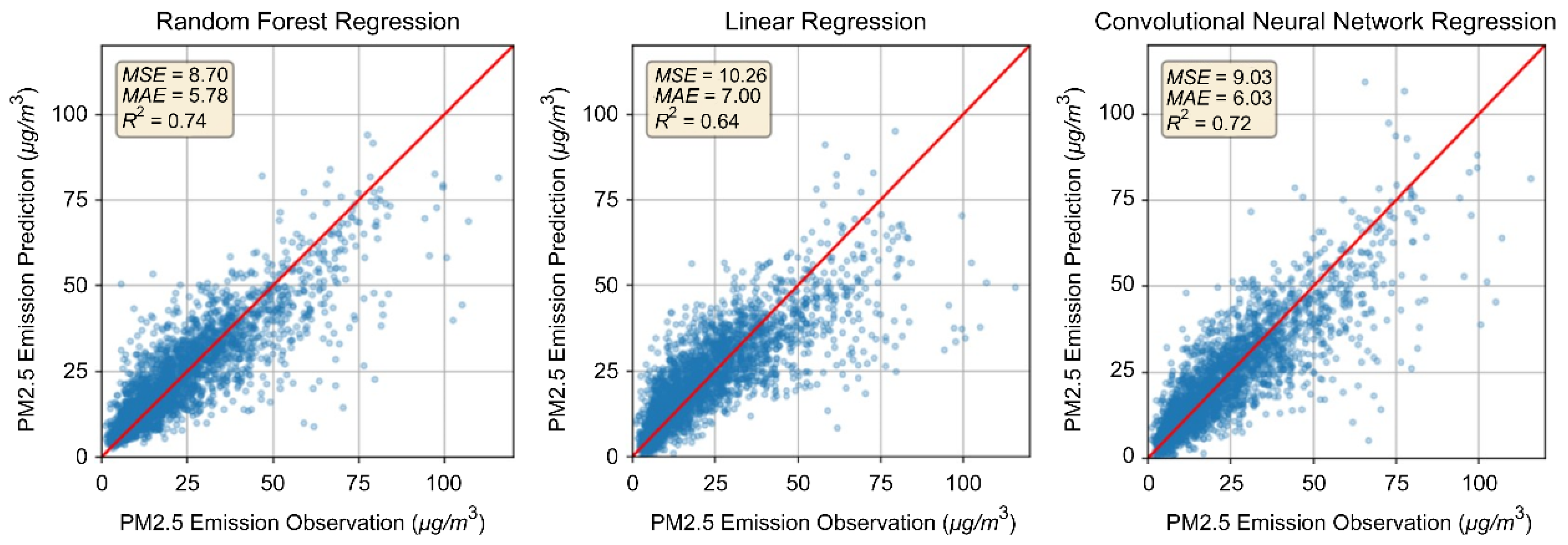
summarizes the performances of the PM_2.5 concentration estimation models for road sections. R² was 0.64 for the linear regression, 0.74 for the random forest, and 0.74 for the convolutional neural network. The random forest model exhibited the highest explanatory power, which was approximately 0.02–0.1 higher than those of the other models.

The MAE was 7.0 for linear regression, 5.78 for random forest, and 6.03 for the convolutional neural network, indicating that the MAE was lowest in the random forest model. The MSE and RMSE were lowest—8.69 and 2.95, respectively—when the random forest model was applied. The PM_2.5 analysis results for road sections indicate that the highest model fit occurred when the random forest model was applied.

The predictive performance of the PM_2.5 concentration estimation models are expressed as scatter plots of the observed and predicted values, as shown in Figure 2. The random forest model showed the best performance.

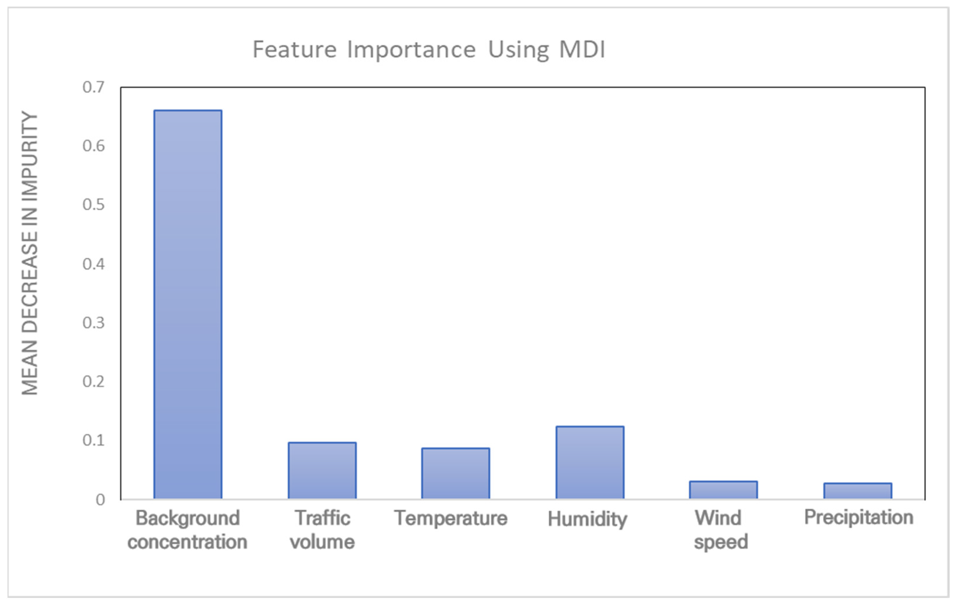
The mean decrease in impurity (MDI) is the number of times a function is used to divide variables, and weights are applied according to the number of divided samples. It is the impact calculated with the statistics obtained from the training dataset; thus, identifying the change in the impact of variables in the test dataset is unfeasible. An unimportant variable in the test data can be the most important variable in the learning process. Figure 3 presents the importance of the variables in the PM_2.5 concentration estimation models.

Previous studies focused on identifying the correlations among variables (e.g., analysis of positive or negative correlations between PM concentrations and explanatory variables). This study contributes a theoretical basis for identifying the relative importance of various explanatory variables. An examination of the importance of variables in the PM_2.5 concentration estimation models revealed that the background concentration had the highest MDI value (0.67). Thus, this variable exhibited the strongest predictive power, followed by humidity (0.124), traffic volume (0.097), and temperature (0.087).

In other words, in the sphere of road pollutants, PM_2.5 concentrations are most significantly affected by the spatiotemporal distribution (i.e., background concentration) of macroscopic PM_2.5 concentrations. Humidity had the largest effect among the local weather factors that determine PM_2.5 concentrations, followed by the effect of the traffic volume, which was important in determining PM_2.5 concentrations from traffic phenomena or road traffic pollutants.

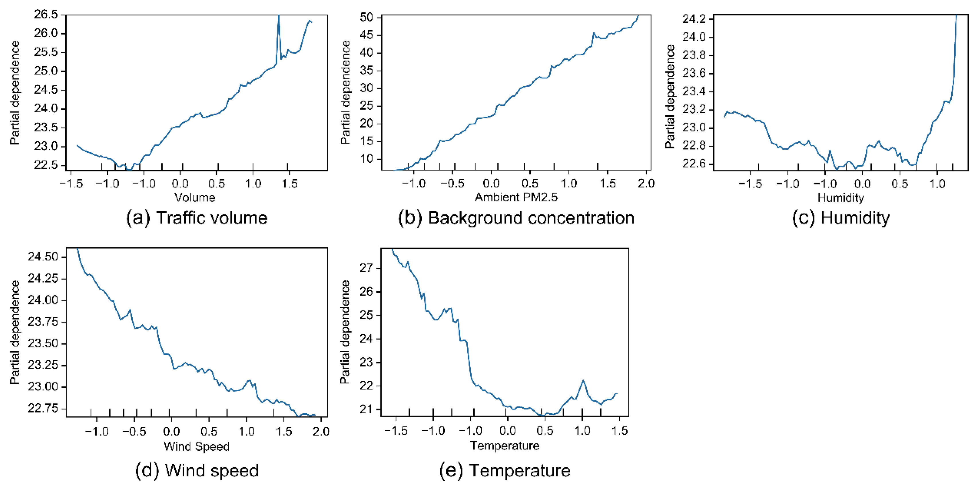
Partial dependence plots (PDPs), shown in Figure 4, were analyzed to determine the correlations between individual factors and PM_2.5 concentrations. In Figure 4, the X-axis variables were normalized to facilitate the analysis of the results.

The PDPs reveal that the traffic volume and background concentration are positively correlated with PM_2.5 (upward-sloping graph), whereas the temperature and wind speed are negatively correlated (downward-sloping graph). Humidity shows a weak positive correlation. These findings are consistent with the literature review (Table 2).

4.3. Construction and Predictive Performance of PM₁₀ Concentration Estimation Models

Table 6. PM₁₀ concentration estimation performance of the different models.

Model	R2	MAE	MSE	RMSE
Linear regression	0.38	14.18	22.73	4.77
Random forest	0.71	9.60	15.51	3.94
Convolutional neural network	0.64	11.58	17.68	4.20

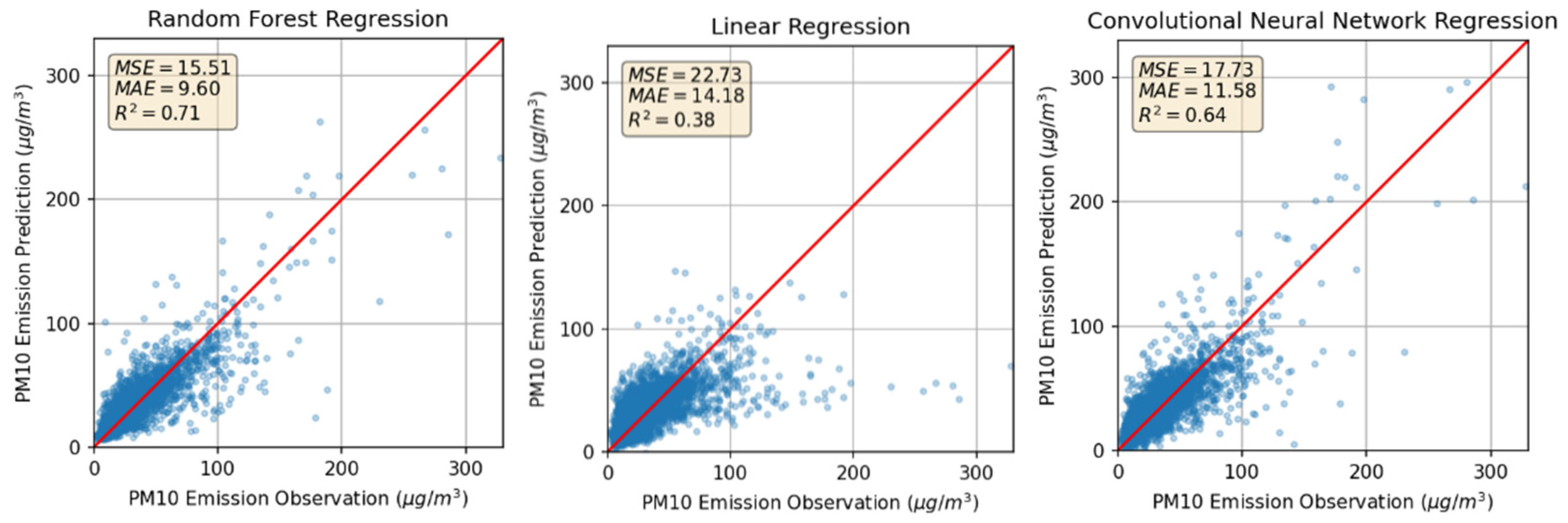
summarizes the performances of the PM₁₀ concentration estimation models for road sections. The random forest model had the highest coefficient of determination (R² = 0.71), which was approximately 0.07–0.3 higher than those of the models constructed with linear regression (0.38) and convolutional neural networks (0.64). These results are similar to those for the PM_2.5 concentration estimation models where the random forest model was optimal.

The random forest model had the lowest MAE (9.60), followed by the convolutional neural network (11.68) and linear regression (14.18). The MAE of the random forest model was approximately 2.0–4.5 lower than those of the other models. The MSE was 22.73 for linear regression, 15.51 for the random forest, and 17.68 for the convolutional neural network. The random forest model also had the lowest RMSE (3.94). Therefore, the random forest model is the most suitable for estimating the PM₁₀ concentration.

The PM10 concentration estimation models were analyzed using scatter plots, which revealed that the random forest model had the best predictive performance (Figure 5).

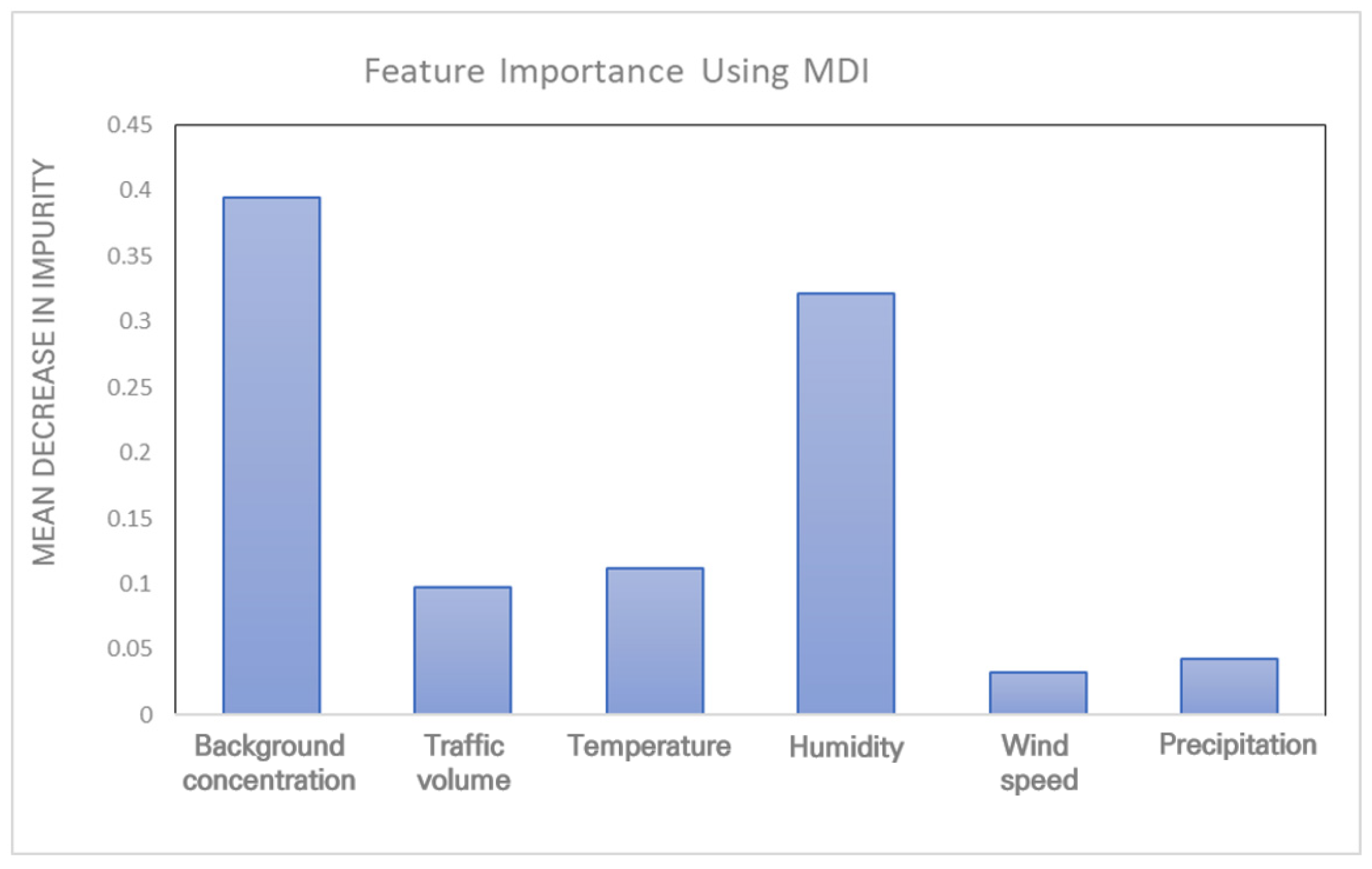
Figure 6 shows the importance of variables in the PM₁₀ concentration estimation models. The background concentration exhibited the highest importance (0.395) for the PM₁₀ concentration estimation models, followed by humidity (0.321), temperature (0.112), and traffic volume (0.096). These results are generally similar to those of the PM_2.5 concentration estimation models. However, the influence of the spatiotemporal distribution of macroscopic PM₁₀ concentrations was relatively low, whereas that of the other local weather and traffic phenomena was relatively high. Among the local weather factors that determined the PM₁₀ concentrations in road sections, humidity had a relatively high effect, whereas the traffic volume had a relatively low effect. The impacts of the background concentration and humidity were high, possibly because natural soil components were included owing to the nature of PM₁₀.

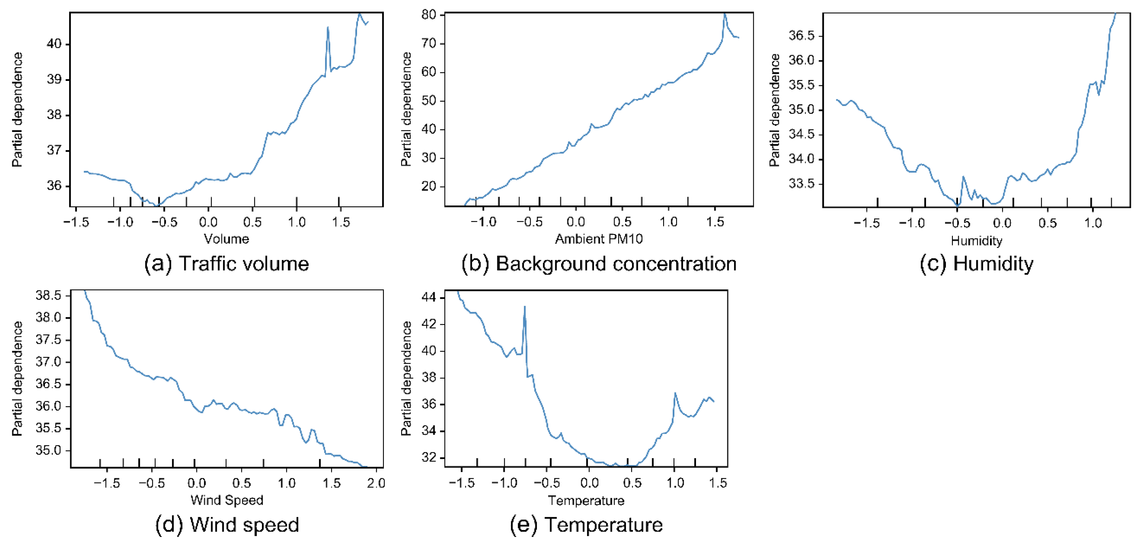
PDPs were analyzed to identify the correlations between individual factors and PM₁₀ concentrations (Figure 7). The PDPs revealed that the traffic volume and background concentration are positively correlated with PM₁₀, whereas temperature and wind speed are negatively correlated. Humidity shows a weak positive correlation. These findings are similar to those for the random forest PM_2.5 estimation model.

The PDP analysis results reveal that the correlations are similar to those for PM_2.5, indicating that the model reflects the relationships well.

5. Model Transferability Verification

Model transferability at the monitoring points was verified for the PM_2.5 and PM₁₀ concentration estimation models.

5.1. Verification Method

Models were constructed using the data from monitoring point 1 (training data) and applied using monitoring point 2 data. Machine learning was used to verify the reliability of the constructed models through model transferability verification. The random forest models had the highest predictive power among the PM_2.5 and PM₁₀ concentration estimation models.

5.2. PM_2.5 Model Transferability Verification Results

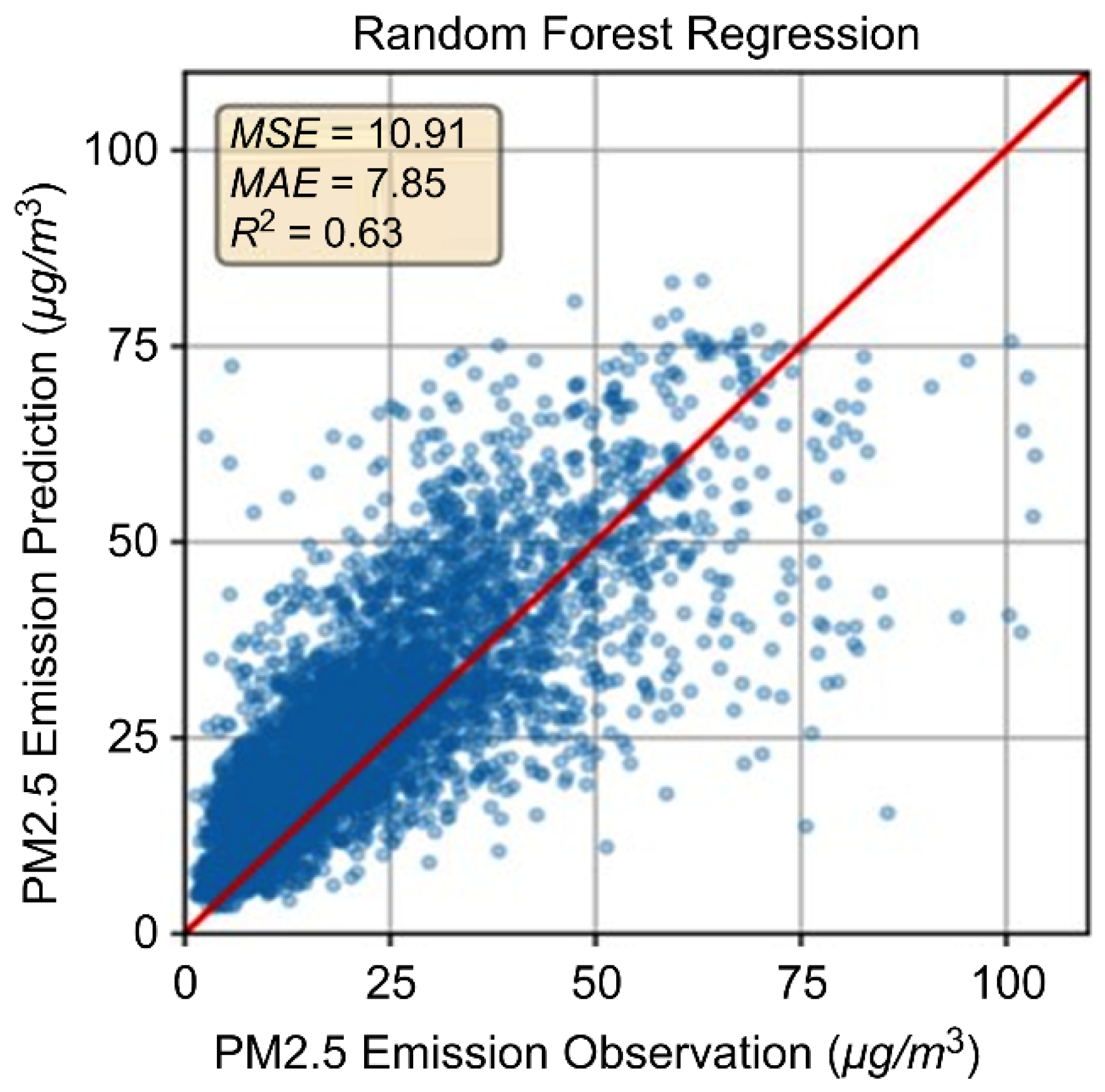
The PM_2.5 model had high explanatory power with an R² of 0.63, indicating the reliability of the PM_2.5 concentration estimation model. The errors in the transferability verification model were low, with an MAE value of 7.85, MSE value of 10.91, and RMSE value of 3.03.

Table 7. PM_2.5 model transferability verification results.

Model	PM2.5
	R2	MAE	MSE	RMSE
Random forest	0.628	7.85	10.91	3.03

summarizes the PM_2.5 model transferability verification results. The scatter plot of the PM_2.5 transferability verification results, shown in Figure 8, indicates the good transferability of the PM_2.5 model.

5.3. PM₁₀ Model Transferability Verification Results

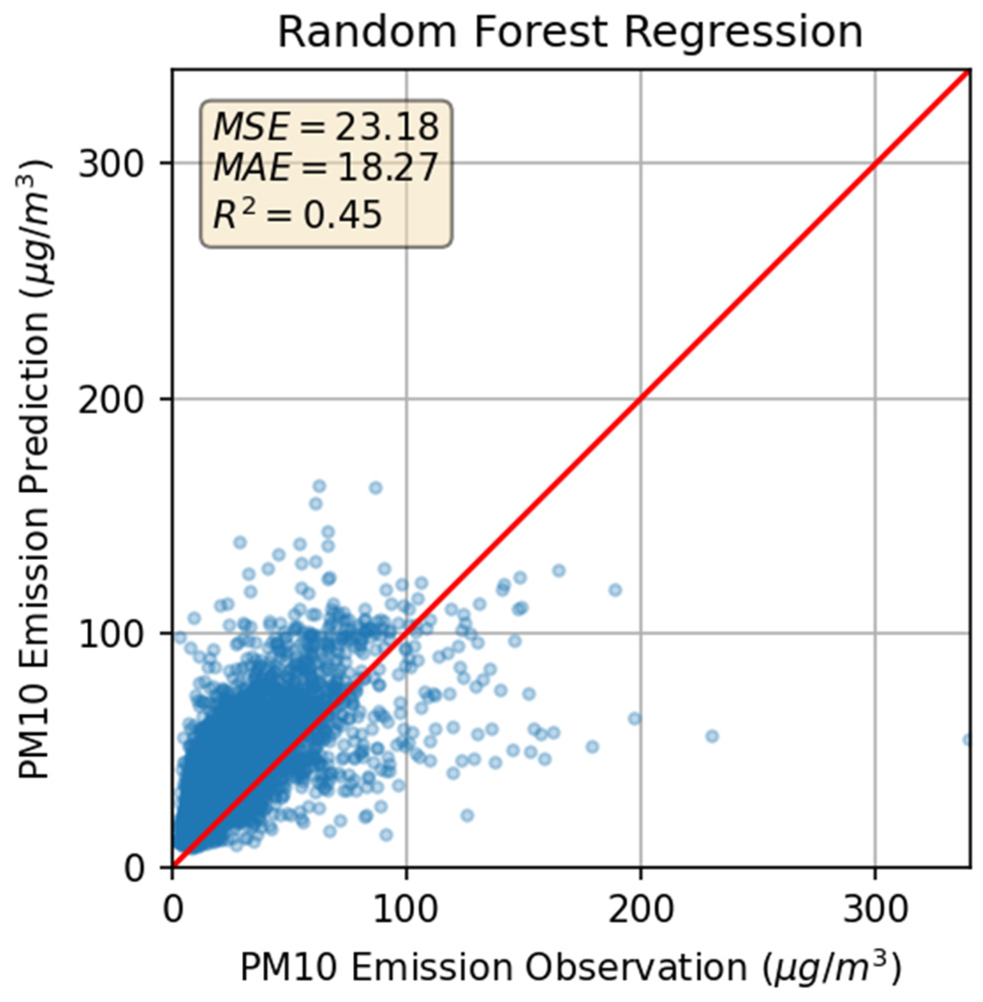
The PM₁₀ model transferability verification revealed relatively low explanatory power (Figure 9), with R² = 0.45, indicating the strong influence of relatively fluctuating environmental factors.

For the transferability verification model, the predicted and observed values had large errors compared to those for the PM_2.5 concentration estimation model. The performance metrics are summarized in

Table 8. PM₁₀ model transferability verification results.

Model	PM10
	R2	MAE	MSE	RMSE
Random forest	0.45	18.27	23.18	4.82

. Although the transferability of the PM₁₀ model was not as good as that for the PM_2.5 model, in the near future, more sensors and monitoring points can be installed so that granular changes in weather and traffic conditions unique to one location can be measured, collected, and used for building the models.

6. Conclusions

In this study, raw data were collected every 5 min by installing traffic volume and PM sensors at road monitoring points. The correlations among the micro-data-based traffic volume, weather, and background concentration variables for PM_2.5 and PM₁₀ concentrations were analyzed, and a sensitivity analysis was performed. Accordingly, models for estimating PM_2.5 and PM₁₀ concentrations in road sections were developed, and transferability verification was performed for these models.

The random forest models had the lowest errors among the PM_2.5 and PM₁₀ concentration estimation models for road sections. In addition, practical utilization methods for the developed models were presented.

This study provides practitioners and policymakers with an accurate and simple model for estimating the concentration of pollutants generated by the transportation sector, thus contributing to the development of regulations and standards for reducing PM.

Although regional PM concentrations are monitored, the effects of traffic regulation policies based on these predictions remain unknown. More detailed traffic regulation policies that reflect the characteristics of each section and region are needed, along with an effectiveness analysis to verify these policies. The PM_2.5 and PM₁₀ concentration estimation models developed in this study are expected to be reflected in future PM reduction policies.

The methodology proposed in this study can also be applied to predict the concentrations of other road traffic pollutants. For example, Korea’s preliminary feasibility study estimates the emissions of four major pollutants (CO, HC, NO_x, and PM), whereas the U.S. Environmental Protection Agency estimates the concentrations of six major pollutants (CO, lead, ozone, PM, NO₂, and SO₂). If a data collection system for other pollutants is established in the future, the methodology described in this study can be applied to build a reliable model for predicting different pollutant levels.