Analytical Model for Rate Transient Behavior of Co-Production between Coalbed Methane and Tight Gas Reservoirs

Abstract

Due to complex geological structures and potential environmental impacts, single-well production in coal-measure gas reservoirs is not satisfactory. Field studies have shown that co-production is a promising approach, which can efficiently and economically extract multiple gas resources. However, the literature lacks a mathematical model to accurately describe and predict the production behavior during co-production. Based on the five-linear flow model, this work presents an analytical solution to evaluate the production dynamics characteristics of co-production between coalbed methane and tight gas reservoirs. In addition, the proposed model accounts for factors such as dual-porosity media, the gas slippage effect, and the matrix shrinkage effect. With the aid of the model, sensitivity analyses of the Blasingame decline curve and the layered flux contribution are conducted. The calculation results show that a higher fracture conductivity, as well as a longer fracture length, lead to larger cumulative production. Additionally, increased layer thickness significantly boosts flux contribution throughout the production period. Finally, large boundary distances extend the duration of high flux contributions in late production. This research contributes to a better understanding of the production dynamics in coal-measure gas reservoirs and offers practical guidelines for reservoir management in co-production scenarios.

1. Introduction

Coal-measure natural gas resources, including coalbed methane, tight gas, and shale gas, have emerged as crucial components of the global energy portfolio. As conventional fossil fuel reserves decrease and concerns about climate change intensify, coal-measure gas is regarded as a crucial alternative, offering a lower-carbon solution to meet growing energy demands [1,2,3]. Countries like the United States, China, and Australia have already made significant investments in developing these resources, positioning coal-measure gas as a key player in the transition to sustainable energy systems [4,5,6]. In China, the total annual production of the Ordos Basin and Qinshui Basin is 96.1 × 10⁸ m³, accounting for 83.2% of the total production of coalbed methane gas [7]. It is worth noting that the coal-measure reservoir is mainly formed in a marine-terrigenous or terrestrial environment with multiple lithological sedimentary. Due to the complex geological conditions, different lithological layers are superimposed on each other, forming strong heterogeneous reservoirs [8]. In real production, the development of this multi-superimposed reservoir is still dominated by a single unconventional gas resource. However, the single-well productivity of this production mode is low, and the economic benefits are not obvious [9]. For instance, the tight gas well typically has a short production life and a faster decline in production [10]; the coalbed methane development exhibits a long production period and requires fracturing to achieve production capacity [11]. Co-production maximizes the extraction of available energy resources from multilayered formations, reducing waste and enhancing overall efficiency. By extracting coalbed methane and tight gas simultaneously, operators can minimize the environmental footprint associated with multiple separate operations. Thus, to improve economic benefits and promote sustainable resource management, the co-production of multi-superimposed gas reservoirs has gradually received significant attention [12].

The co-production of multi-superimposed gas reservoirs is an emerging engineering technology with significant potential [13,14]. Due to the high difficulty and development costs of shale gas exploitation, coal-measure gas is primarily focused on the co-production of coalbed methane and tight gas. Preliminary applications and research have been conducted in North America, China, and other resource-rich areas [15,16]. Although it is currently in its early stages of development, its application prospects will become increasingly promising with continuous technological advancements and in-depth research. In the existing literature, Ou et al. [17] developed a comprehensive evaluation method for heterogeneous multilayer sandstone gas reservoirs. Guo et al. [18] introduced a semi-analytical model to evaluate stress-sensitive multilayer carbonate gas reservoirs, addressing challenges from complex sedimentary environments. Zhong et al. [19] proposed the Co-production Compatibility Index, evaluated factors affecting multilayer co-production in tight gas reservoirs through simulations, and validated its applicability in the Daning–Jixian gas field. Lu et al. [20] presented a new solution for pressure transient behavior in multilayer reservoirs with crossflow, solving pressure dynamics analytically for fully penetrating vertical wells. Zhang et al. [21] identified five potential interlayer interference types in multilayer tight gas reservoirs, analyzing their impact through reservoir and pore-scale simulations. In the above studies, the transient flow behavior in multilayer reservoirs of the same type of gas is the focus of research. At present, the studies on the production dynamic characteristics of multi-superposed gas reservoirs are inadequate. For example, Huang and Wang [22] analyzed the co-production of coal-measure gas, highlighting key control factors, optimization strategies, and recovery improvements in Well X, Ordos Basin. Zhao et al. [14] explored the co-production of tight gas and coalbed methane, identifying optimal reservoir combinations and key factors affecting gas production. Based on the above-mentioned studies, several main problems associated with co-production in coal-measure gas reservoirs are listed in

Table 1. Main problems associated with co-production in coal-measure gas reservoirs.

Number	Problem Literary	Problem Literary
1	Spatial distribution problem	[4,5,6,7,8]
2	Single-layer production problem	[9,10,11]
3	Co-production challenge	[12,13,14,15,16,17,18,19,20,21,22]

. As one can see, there is a lack of in-depth research on the impact of transient rate behavior on production.

Moreover, numerical modeling is a powerful tool for understanding gas flow dynamics through rock formations, particularly for methane in coalbed methane and tight gas reservoirs. It helps simulate complex flow mechanisms, such as gas desorption, diffusion, and seepage within heterogeneous geological formations. However, the numerical method is time-consuming and inconvenient in simulating numerous field cases. Therefore, this work proposes an analytical model to investigate the transient rate behavior of co-production between coalbed methane and tight gas reservoirs. Subsequently, based on the Blasingame decline analysis theory, key reservoir parameters that influence the overall performance of the co-production system are analyzed. In addition, the flux contribution of a tight gas layer is investigated to understand trends in production over time. This research will facilitate the estimation of reserves, production forecasting, and optimization of production strategies, thereby enhancing the economic viability and operational efficiency of co-producing coalbed methane and tight gas reservoirs.

2. Methodology

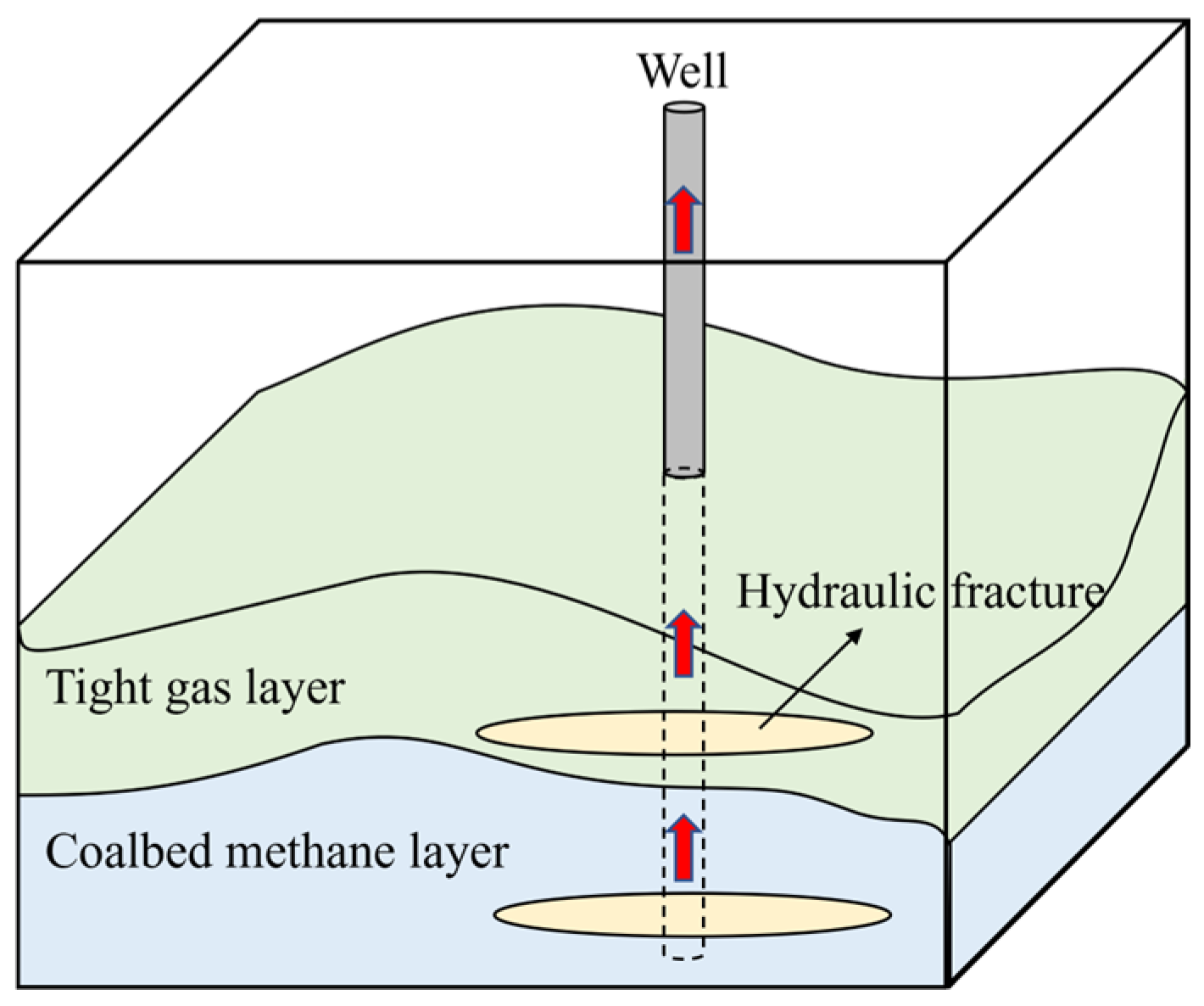
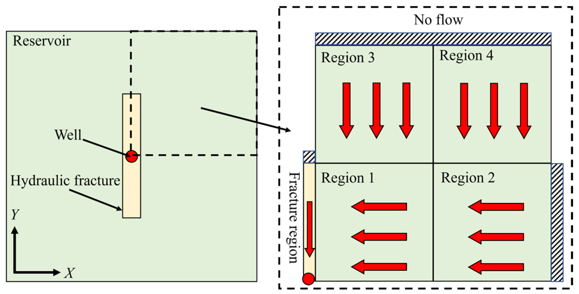
2.1. Physical Model

In a multi-superimposed gas system, it is common to observe a vertical distribution where a tight sandstone layer is found above and a coalbed methane layer below. In order to intuitively understand the geological conditions and production conditions, Figure 1 shows a schematic of the co-production between coalbed methane and tight gas reservoirs. The wellbore penetrates multiple gas-bearing formations, allowing for the simultaneous extraction of gas from both types of reservoirs. In addition, hydraulic fracturing technology is used to retrofit reservoirs to increase productivity. During production, the natural gas flows from the reservoir to the fracture and then into the wellbore. To construct an analytical model, the other basic assumptions are listed below:

• The dual porosity media is considered in the tight gas reservoir;
• The effect of gas slippage and matrix shrinkage is considered in the coalbed methane;
• There are interlayers between each layer, not communicating with each other;
• The properties of tight gas and coalbed methane reservoirs are assumed to be isotropic;
• The natural gas is produced with constant pressure;
• The gravity and temperature effects are neglected in this simulation.

2.2. Mathematical Model

According to the symmetry of the model, 1/4 of the hydraulic fracture in one layer is taken as the research object (as shown in Figure 2). To accurately describe the reservoir heterogeneity caused by fracturing, the flow behavior in a simulated region is regarded as a combination of five linear flows. Specifically, the fluid within region 3 and region 4 flows along the y-direction; the fluid within region 1 and region 2 flows along the x-direction; then, the fluid from the reservoir linearly flows into the wellbore through the fracture region.

In addition, the effective compressibility of gas considering the matrix shrinkage effect can be obtained from the following [23]:

$$C_d={\displaystyle \frac{P_{sc}{V}_L{P}_{L}TZ}{\varphi P{T}_{sc}{Z}_{sc}{(P_L+P)}^2}}$$

(1)

where P_sc is the pressure under the standard condition, V_L is the Langmuir volume, P_L is the Langmuir pressure, T is the temperature, Z is the compressibility factor, ϕ is the porosity, P is the pressure, and Z_sc is the compressibility factor under the standard condition. The apparent permeability subject to the gas slippage effect can be obtained from the following [24]:

$$k_a=\left(1+{\displaystyle \frac{\mu c_g{D}_g}{k}}\right)k$$

(2)

where µ is the gas viscosity, c_g is the gas compressibility, D_g is the gas diffusion coefficient, and k is the initial permeability. Based on the study of Stalgorova and Mattar [25], the governing equations for each region are derived. By introducing pseudo-pressure and pseudo-time into the governing equations, the pressure distribution in region 4 can be expressed as follows:

$$\left\{\begin{array}{cc}{\displaystyle \frac{{\partial }^2\mathsf{\Delta }{m}_4}{\partial y^2}}={\displaystyle \frac{1}{{\eta }_4}}{\displaystyle \frac{\partial \mathsf{\Delta }{m}_4}{\partial t}}\hfill & \left(\mathrm{Matrix}\right)\hfill \\ {\left.\mathsf{\Delta }{m}_4\right|}_{y=y_1}={\left.\mathsf{\Delta }{m}_2\right|}_{y=y_1}\hfill & (\mathrm{Inner} \mathrm{boundary} \mathrm{condition})\hfill \\ {\left.{\displaystyle \frac{\partial \mathsf{\Delta }{m}_4}{\partial y}}\right|}_{y=y_2}=0\hfill & (\mathrm{Outer} \mathrm{boundary} \mathrm{condition})\hfill \\ {\left.\mathsf{\Delta }{m}_4\right|}_{t=0}=0\hfill & (\mathrm{Initial} \mathrm{condition})\hfill \end{array}\right.$$

(3)

where Δm is the difference between the current pseudo-pressure and the initial pseudo-pressure, η is the diffusivity coefficient, defined as η = k/µc_tϕ, y₁ is the y-coordinate of the inner boundary of region 4, y₂ is the y-coordinate of the outer boundary of region 4, and t is the material balance pseudo-time. The pressure distribution in region 3 can be expressed as follows:

$$\left\{\begin{array}{cc}{\displaystyle \frac{{\partial }^2\mathsf{\Delta }{m}_3}{\partial y^2}}={\displaystyle \frac{1}{{\eta }_3}}{\displaystyle \frac{\partial \mathsf{\Delta }{m}_3}{\partial t}}\hfill & \left(\mathrm{Matrix}\right)\hfill \\ {\left.\mathsf{\Delta }{m}_3\right|}_{y=y_1}={\left.\mathsf{\Delta }{m}_1\right|}_{y=y_1}\hfill & (\mathrm{Inner} \mathrm{boundary} \mathrm{condition})\hfill \\ {\left.{\displaystyle \frac{\partial \mathsf{\Delta }{m}_3}{\partial y}}\right|}_{y=y_2}=0\hfill & (\mathrm{Outer} \mathrm{boundary} \mathrm{condition})\hfill \\ {\left.\mathsf{\Delta }{m}_3\right|}_{t=0}=0& (\mathrm{Initial} \mathrm{condition})\hfill \end{array}\right.$$

(4)

The pressure distribution in region 2 can be expressed as follows:

$$\left\{\begin{array}{l}{\displaystyle \frac{{\partial }^2\mathsf{\Delta }{m}_2}{\partial x^2}}+{\displaystyle \frac{k_4}{k_2{y}_1}}{\left.{\displaystyle \frac{\partial \mathsf{\Delta }{m}_4}{\partial y}}\right|}_{y=y_1}={\displaystyle \frac{1}{{\eta }_2}}{\displaystyle \frac{\partial \mathsf{\Delta }{m}_2}{\partial t}} \left(\mathrm{Matrix}\right)\hfill \\ {\left.\mathsf{\Delta }{m}_2\right|}_{x=x_1}={\left.\mathsf{\Delta }{m}_1\right|}_{x=x_1} \hspace{1em}\hspace{1em}\hspace{1em}\hspace{1em}\hspace{1em}\hspace{1em}\hspace{1em} (\mathrm{Inner} \mathrm{boundary} \mathrm{condition})\hfill \\ {\left.{\displaystyle \frac{\partial \mathsf{\Delta }{m}_2}{\partial x}}\right|}_{x=x_2}=0 \hspace{1em}\hspace{1em}\hspace{1em}\hspace{1em}\hspace{1em}\hspace{1em}\hspace{1em}\hspace{1em}\hspace{1em} (\mathrm{Outer} \mathrm{boundary} \mathrm{condition})\hfill \\ {\left.\mathsf{\Delta }{m}_2\right|}_{t=0}=0 \hspace{1em}\hspace{1em}\hspace{1em}\hspace{1em}\hspace{1em}\hspace{1em}\hspace{1em}\hspace{1em}\hspace{1em}\hspace{1em} (\mathrm{Initial} \mathrm{condition})\hfill \end{array}\right.$$

(5)

where x₁ is the x-coordinate of the inner boundary of region 2, and x₂ is the x-coordinate of the outer boundary of region 2. In this work, region 1 in the tight gas and coalbed methane layers is considered a dual-porosity medium and a single-porosity medium, respectively. This is because tight gas reservoirs are characterized by their complex pore structures, including micro-pores and macro-fractures, which significantly impact fluid flow behavior. The dual-porosity medium model is well-suited to capture these dynamics [24]. Thus, the governing equations in region 1 and the fracture region in the tight gas layer are different from those in the coalbed methane layer. In terms of the tight gas layer, the pressure distribution in region 1 can be expressed as follows:

$$\left\{\begin{array}{l}{\displaystyle \frac{{\partial }^2\mathsf{\Delta }{m}_{nf}}{\partial x^2}}+{\displaystyle \frac{k_3}{k_{nf}{y}_1}}{\left.{\displaystyle \frac{\partial \mathsf{\Delta }{m}_3}{\partial y}}\right|}_{y=y_1}+\alpha {\displaystyle \frac{k_1}{k_{nf}}}\left(\mathsf{\Delta }{m}_m-\mathsf{\Delta }{m}_{nf}\right)={\displaystyle \frac{1}{{\eta }_{nf}}}{\displaystyle \frac{\partial \mathsf{\Delta }{m}_{nf}}{\partial t}}\hspace{1em} (\mathrm{Natural} \mathrm{fracture})\\ \alpha \left(\mathsf{\Delta }{m}_m-\mathsf{\Delta }{m}_{nf}\right)={\displaystyle \frac{1}{{\eta }_m}}{\displaystyle \frac{\partial \mathsf{\Delta }{m}_m}{\partial t}}\hspace{1em}\hspace{1em}\hspace{1em}\hspace{1em}\hspace{1em}\hspace{1em}\hspace{1em}\hspace{1em}\hspace{1em}\hspace{1em}\hspace{1em}\hspace{1em}\hspace{1em}\hspace{1em}\left(\mathrm{Matrix}\right)\\ {\left.\mathsf{\Delta }{m}_{nf}\right|}_{x=0}={\left.\mathsf{\Delta }{m}_f\right|}_{x=0}\hspace{1em}\hspace{1em}\hspace{1em}\hspace{1em}\hspace{1em}\hspace{1em}\hspace{1em}\hspace{1em}\hspace{1em}\hspace{1em}\hspace{1em}\hspace{1em}\hspace{1em}\hspace{1em}\hspace{1em}\hspace{1em}\hspace{1em}\hspace{1em}(\mathrm{Inner} \mathrm{boundary} \mathrm{condition})\\ {\left.{\displaystyle \frac{k_{nf}}{\mu }}{\displaystyle \frac{\partial m_{nf}}{\partial x}}\right|}_{x=x_1}={\left.{\displaystyle \frac{k_2}{\mu }}{\displaystyle \frac{\partial m_2}{\partial x}}\right|}_{x=x_1}\hspace{1em}\hspace{1em}\hspace{1em}\hspace{1em}\hspace{1em}\hspace{1em}\hspace{1em}\hspace{1em}\hspace{1em}\hspace{1em}\hspace{1em}\hspace{1em}\hspace{1em}\hspace{1em}(\mathrm{Outer} \mathrm{boundary} \mathrm{condition})\\ {\left.\mathsf{\Delta }{m}_{nf}\right|}_{t=0}=0\hspace{1em}\hspace{1em}\hspace{1em}\hspace{1em}\hspace{1em}\hspace{1em}\hspace{1em}\hspace{1em}\hspace{1em}\hspace{1em}\hspace{1em}\hspace{1em}\hspace{1em}\hspace{1em}\hspace{1em}\hspace{1em}\hspace{1em}\hspace{1em}\hspace{1em}\hspace{1em} (\mathrm{Initial} \mathrm{condition})\end{array}\right.$$

(6)

where α is the geometric parameter for the heterogeneous region. Note that Δm_nf in Equation (6) is the same as Δm₁ in Equations (3) and (4). The pressure distribution in the fracture region can be expressed as follows:

$$\left\{\begin{array}{l}{\displaystyle \frac{{\partial }^2\mathsf{\Delta }{m}_f}{\partial y^2}}+{\displaystyle \frac{2k_{nf}}{k_f{w}_f}}{\left.{\displaystyle \frac{\partial \mathsf{\Delta }{m}_{nf}}{\partial x}}\right|}_{x=0}={\displaystyle \frac{1}{{\eta }_f}}{\displaystyle \frac{\partial \mathsf{\Delta }{m}_f}{\partial t}}\hspace{1em}(\mathrm{Artificial} \mathrm{fracture})\\ {\left.\mathsf{\Delta }{m}_f\right|}_{y=0}=\mathsf{\Delta }{m}_c\hspace{1em}\hspace{1em}\hspace{1em}\hspace{1em}\hspace{1em}\hspace{1em}\hspace{1em}\hspace{1em}\hspace{1em} (\mathrm{Inner} \mathrm{boundary} \mathrm{condition})\\ {\left.{\displaystyle \frac{\partial \mathsf{\Delta }{m}_f}{\partial y}}\right|}_{y=y_1}=0\hspace{1em}\hspace{1em}\hspace{1em}\hspace{1em}\hspace{1em}\hspace{1em}\hspace{1em}\hspace{1em}\hspace{1em} (\mathrm{Outer} \mathrm{boundary} \mathrm{condition})\\ {\left.\mathsf{\Delta }{m}_f\right|}_{t=0}=0\hspace{1em}\hspace{1em}\hspace{1em}\hspace{1em}\hspace{1em}\hspace{1em}\hspace{1em}\hspace{1em}\hspace{1em}\hspace{1em} (\mathrm{Initial} \mathrm{condition})\end{array}\right.$$

(7)

where w_f is the hydraulic fracture width, and Δm_c is the constant pressure condition. In terms of the coalbed methane layer, Equations (6) and (7) can be rewritten as follows:

$$\left\{\begin{array}{l}{\displaystyle \frac{{\partial }^2\mathsf{\Delta }{m}_1}{\partial x^2}}+{\displaystyle \frac{k_3}{k_1{y}_1}}{\left.{\displaystyle \frac{\partial \mathsf{\Delta }{m}_3}{\partial y}}\right|}_{y=y_1}={\displaystyle \frac{1}{{\eta }_1}}{\displaystyle \frac{\partial \mathsf{\Delta }{m}_1}{\partial t}}\hspace{1em}\left(\mathrm{Matrix}\right)\\ {\left.\mathsf{\Delta }{m}_1\right|}_{x=0}={\left.\mathsf{\Delta }{m}_f\right|}_{x=0}\hspace{1em}\hspace{1em}\hspace{1em}\hspace{1em}\hspace{1em}\hspace{1em}\hspace{1em}\hspace{1em} (\mathrm{Inner} \mathrm{boundary} \mathrm{condition})\\ {\left.{\displaystyle \frac{k_1}{\mu }}{\displaystyle \frac{\partial m_1}{\partial x}}\right|}_{x=x_1}={\left.{\displaystyle \frac{k_2}{\mu }}{\displaystyle \frac{\partial m_2}{\partial x}}\right|}_{x=x_1}\hspace{1em}\hspace{1em}\hspace{1em}\hspace{1em} (\mathrm{Outer} \mathrm{boundary} \mathrm{condition})\\ {\left.\mathsf{\Delta }{m}_1\right|}_{t=0}=0\hspace{1em}\hspace{1em}\hspace{1em}\hspace{1em}\hspace{1em}\hspace{1em}\hspace{1em}\hspace{1em}\hspace{1em}\hspace{1em} (\mathrm{Initial} \mathrm{condition})\end{array}\right.$$

(8)

$$\left\{\begin{array}{l}{\displaystyle \frac{{\partial }^2\mathsf{\Delta }{m}_f}{\partial y^2}}+{\displaystyle \frac{2k_1}{k_f{w}_f}}{\left.{\displaystyle \frac{\partial \mathsf{\Delta }{m}_1}{\partial x}}\right|}_{x=0}={\displaystyle \frac{1}{{\eta }_f}}{\displaystyle \frac{\partial \mathsf{\Delta }{m}_f}{\partial t}}\hspace{1em}(\mathrm{Artificial} \mathrm{fracture})\\ {\left.\mathsf{\Delta }{m}_f\right|}_{y=0}=\mathsf{\Delta }{m}_c\hspace{1em}\hspace{1em}\hspace{1em}\hspace{1em}\hspace{1em}\hspace{1em}\hspace{1em}\hspace{1em}\hspace{1em}(\mathrm{Inner} \mathrm{boundary} \mathrm{condition})\\ {\left.{\displaystyle \frac{\partial \mathsf{\Delta }{m}_f}{\partial y}}\right|}_{y=y_1}=0\hspace{1em}\hspace{1em}\hspace{1em}\hspace{1em}\hspace{1em}\hspace{1em}\hspace{1em}\hspace{1em}\hspace{1em}(\mathrm{Outer} \mathrm{boundary} \mathrm{condition})\\ {\left.\mathsf{\Delta }{m}_f\right|}_{t=0}=0\hspace{1em}\hspace{1em}\hspace{1em}\hspace{1em}\hspace{1em}\hspace{1em}\hspace{1em}\hspace{1em}\hspace{1em}\hspace{1em} (\mathrm{Initial} \mathrm{condition})\end{array}\right.$$

(9)

2.3. Solutions

With the aid of the Laplace transformation, the production rate solution of each layer in the Laplace domain can be obtained as follows (see detailed derivation in Appendix A):

$$\overline{q}={\displaystyle \frac{2\beta T_{sc}{k}_f{w}_{f}h}{T{P}_{sc}}}{\left.{\displaystyle \frac{\partial \mathsf{\Delta }\overline{m}}{\partial y}}\right|}_{y=0}$$

(10)

where β is the unit conversion factor. By using the Stehfest inversion [26], the production rate solution in the Laplace domain can be transferred to that in the real-time domain. The total production rate solution can be obtained by summing up each layer. Subsequently, the parameters for the Blasingame decline analysis (including the normalized rate, the cumulative production, and the integral derivative production) can be calculated as follows:

$$\left\{\begin{array}{l}\mathrm{Normalized} \mathrm{rate}:\hspace{1em}\hspace{1em}\hspace{1em}\hspace{1em}\hspace{1em}\hspace{1em}\hspace{1em}{q}_w={\displaystyle \frac{q}{\mathsf{\Delta }{m}_c}}\hfill \\ \mathrm{Cumulative} \mathrm{production}:\hspace{1em}\hspace{1em}\hspace{1em}\hspace{1em} q_{wi}={\displaystyle \frac{1}{t}}{\displaystyle {\int }_0^t{q}_w}d\tau \hfill \\ \mathrm{Integral} \mathrm{derivative} \mathrm{production}:\hspace{1em} q_{wid}={\displaystyle \frac{d{q}_{wi}}{d\ln t}}\hfill \end{array}\right.$$

(11)

3. Results and Discussion

In this section, the effects of critical parameters on the Blasingame decline type curve and the layered flux contribution are discussed, including the fracture conductivity ratio, the fracture length ratio, the layer thickness ratio, and the boundary distance ratio. The reservoir parameters used for analysis are listed in

Table 2. The reservoir parameters used for analysis in this section.

Parameter		Value	Unit
Tight gas layer	Fracture permeability	1 × 104	mD
	Fracture porosity	0.2	m
	Fracture length	400	m
	Fracture width	0.001	m
	Natural fracture permeability	50	mD
	Natural fracture porosity	0.01
	Permeability of region 1	0.02	mD
	Permeability of regions 2, 3, 4	0.01	mD
	Porosity of region 1	0.2
	Porosity of regions 2, 3, 4	0.01
Coalbed methane layer	Fracture permeability	1 × 104	mD
	Fracture porosity	0.2
	Fracture length	400	m
	Fracture width	0.001	m
	Langmuir volume	10	m3/ton
	Langmuir pressure	3.5	MPa
	Permeability of region 1	0.2	mD
	Permeability of regions 2, 3, 4	0.1	mD
	Porosity of region 1	0.2
	Porosity of regions 2, 3, 4	0.1
Reservoir	Formation thickness	5	m
	x-coordinate of the boundary of region 1	400	m
	x-coordinate of the boundary of region 2	800	m
	y-coordinate of the boundary of region 3	400	m

.

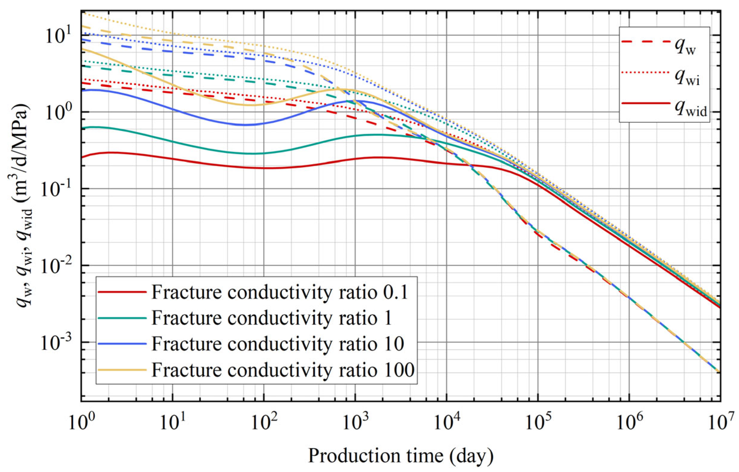
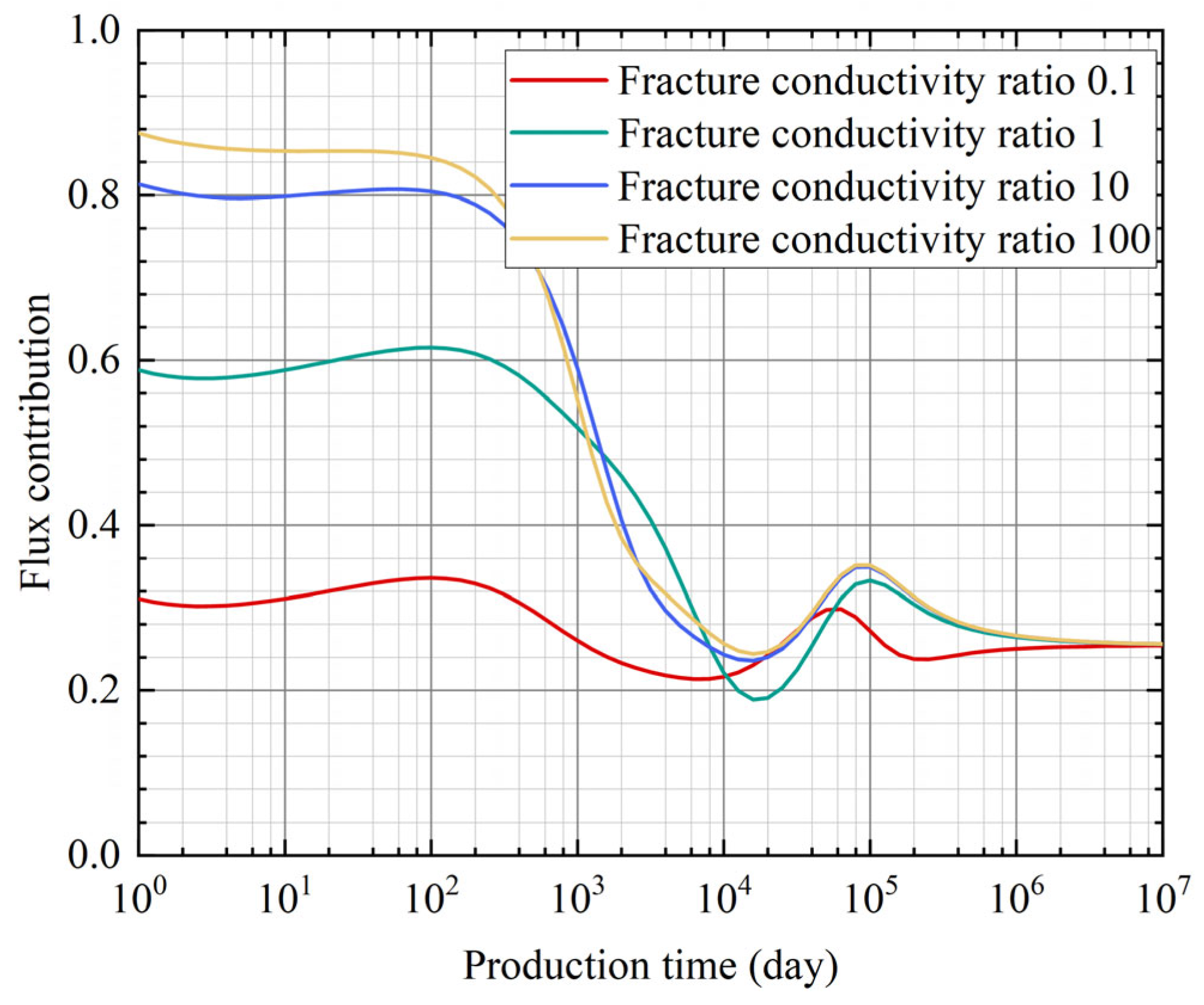
3.1. Fracture Conductivity Ratio

The fracture conductivity is an important parameter in evaluating the efficiency of a hydraulic fracture, as it directly impacts the flow of fluids through the created fracture to the wellbore. In this section, the fracture conductivity ratio is defined as the ratio of fracture conductivity of a tight gas layer to that of a coalbed methane layer. To study the effect of permeability variation between different layers on gas production rate, four fracture conductivity ratios (i.e., 0.1, 1, 10, and 100) are selected for simulation. Figure 3 shows the effect of different fracture conductivity ratios on the Blasingame decline type curve. It can be seen from the figure that the Blasingame decline type curves under different fracture conductivity ratios exhibit large differences in the early and middle production. Three types of curves show a significant rise with the fracture conductivity of the tight gas layer increases. This is because a large fracture conductivity can reduce flow resistance within the system, allowing the well to produce fluids at a higher rate. On the Blasingame curve, this manifests as slower pressure depletion and increased cumulative production.

Figure 4 shows the effect of different fracture conductivity ratios on the flux contribution of the tight gas layer. The flux contribution refers to the contribution of the tight gas layer to the overall flux. The fracture conductivity ratio mainly affects the flux contribution of the tight gas layer in the early production. For example, as the fracture conductivity ratio increases, the flux contribution of the tight gas layer increases from 0.3 to 0.8. However, in the late production, the different fracture conductivity ratios show a slight impact on the flux contribution. The reason is that most of the production comes from the zones near the hydraulic fractures in tight gas reservoirs. Over time, gas in these zones is produced first, while gas farther away from the fractures moves slowly toward the wellbore. Due to the low permeability, it takes longer for gas from the undisturbed reservoir to migrate into the fractures, resulting in a sharp decline in production. Figure 5 shows the production rate of tight gas and coalbed methane layers varies with time under the fracture conductivity ratio 1. Due to the natural fracture of region 1, the tight gas layer exhibits a higher production rate but experiences a more rapid decline compared to the coalbed methane layer. As a result, the resources in the tight gas layer deplete more quickly. However, at the late production, particularly around day 1 × 10⁵, the production rate decline of the tight gas layer slows significantly. This reduced decline leads to an increase in flux contribution from the tight gas layer during this period.

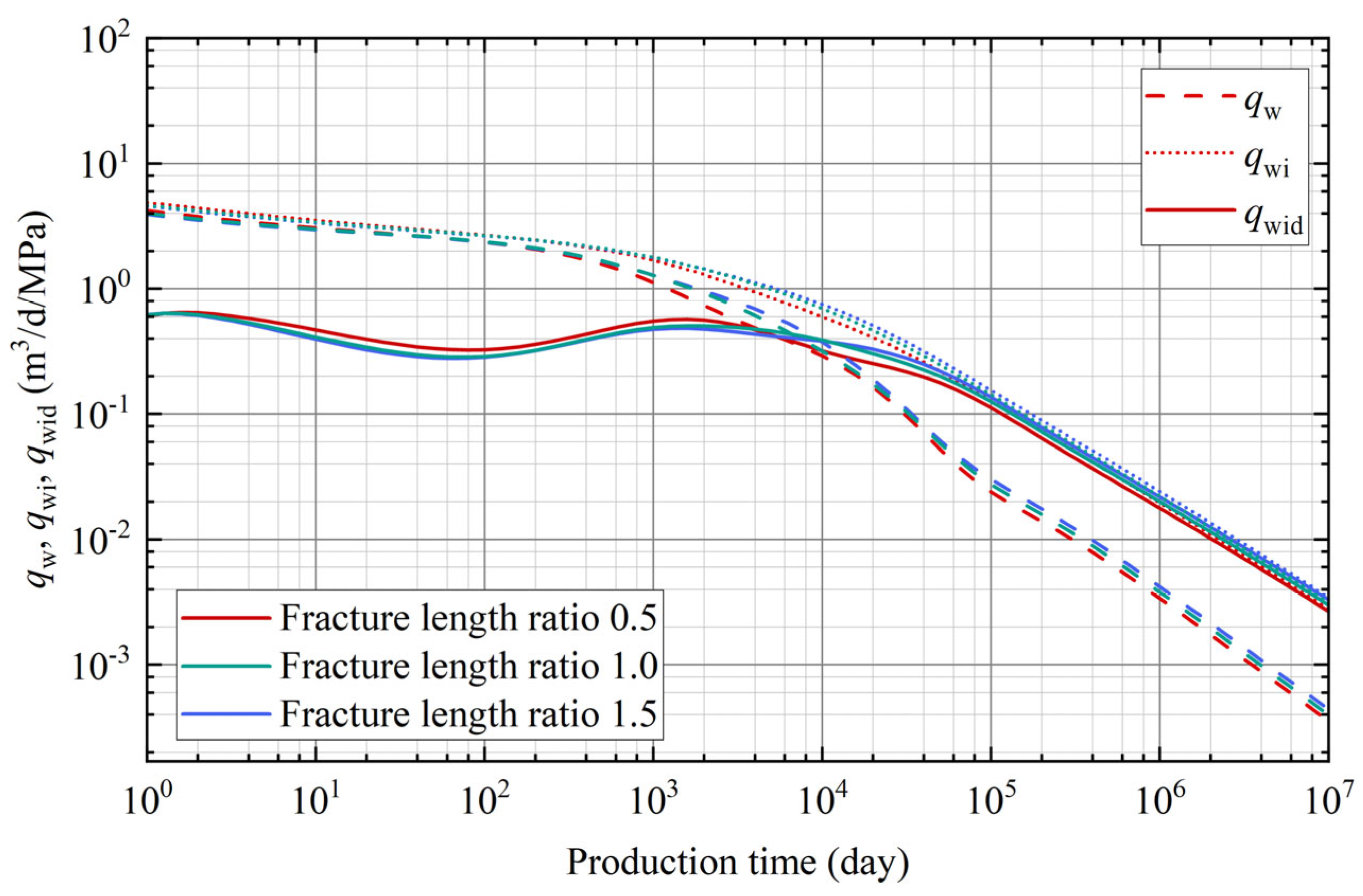
3.2. Fracture Length Ratio

Fracture length is a key determinant of the efficiency and success of hydraulic fracturing operations, influencing both the technical and economic outcomes of hydrocarbon production. Figure 6 shows the effect of different fracture length ratios on the Blasingame decline type curve. The fracture length ratio is defined as the ratio of the fracture length of a tight gas layer to that of a coalbed methane layer. In this figure, the fracture length ratio is varied from 0.5 to 1.5. A longer fracture typically contacts more of the reservoir, leading to higher gas production. In addition, a longer fracture often results in a slower decline rate. This is because longer fractures can drain more reservoir fluid, extending the duration of the high-production phase. Figure 7 shows the effect of different fracture length ratios on the flux contribution of the tight gas layer. It can be found that the fracture length has a significant influence on the flux contribution of the tight gas layer in the middle and late production. Increased fracture length means that more of the reservoir area in the tight gas layer is effectively connected, enhancing the reservoir’s effective permeability. As the pressure in the reservoir gradually decreases over time, a larger portion of the tight gas layer can continue to contribute fluids, maintaining production levels.

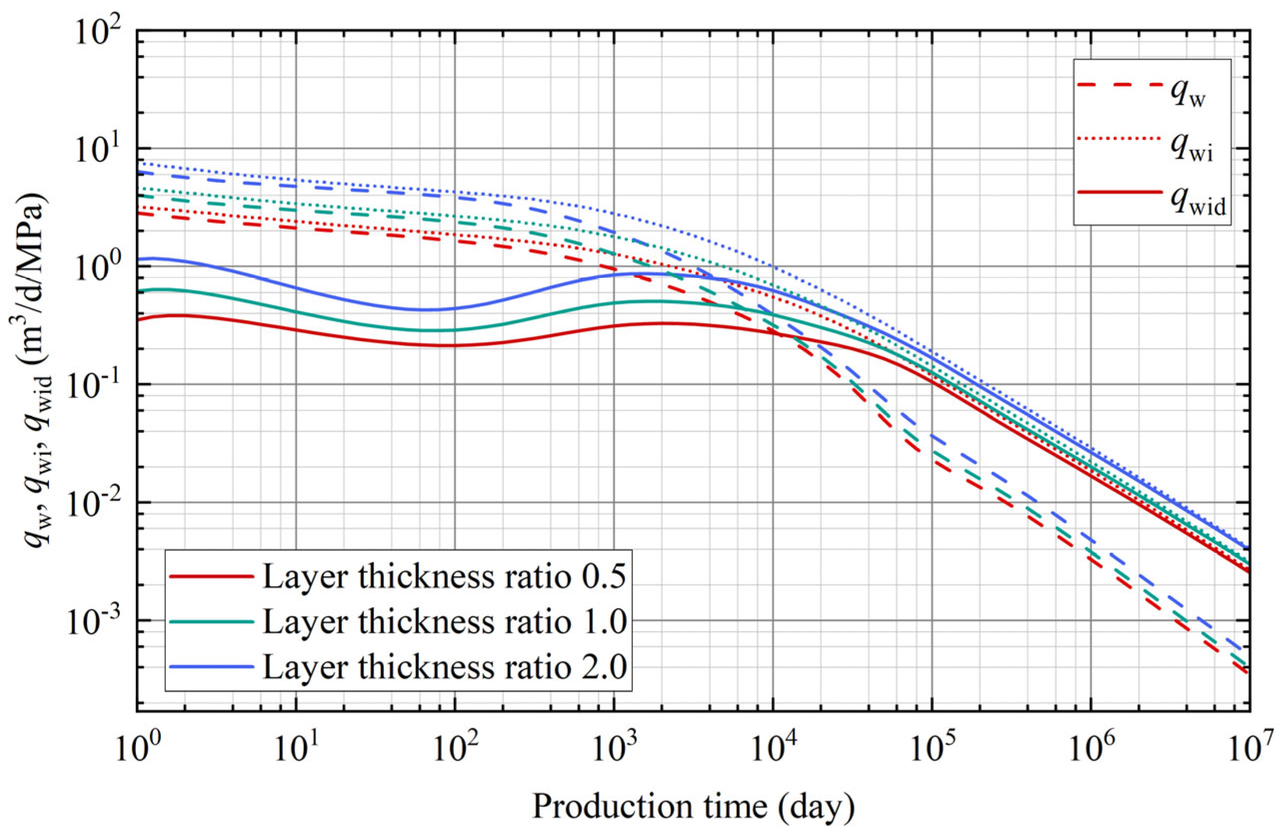
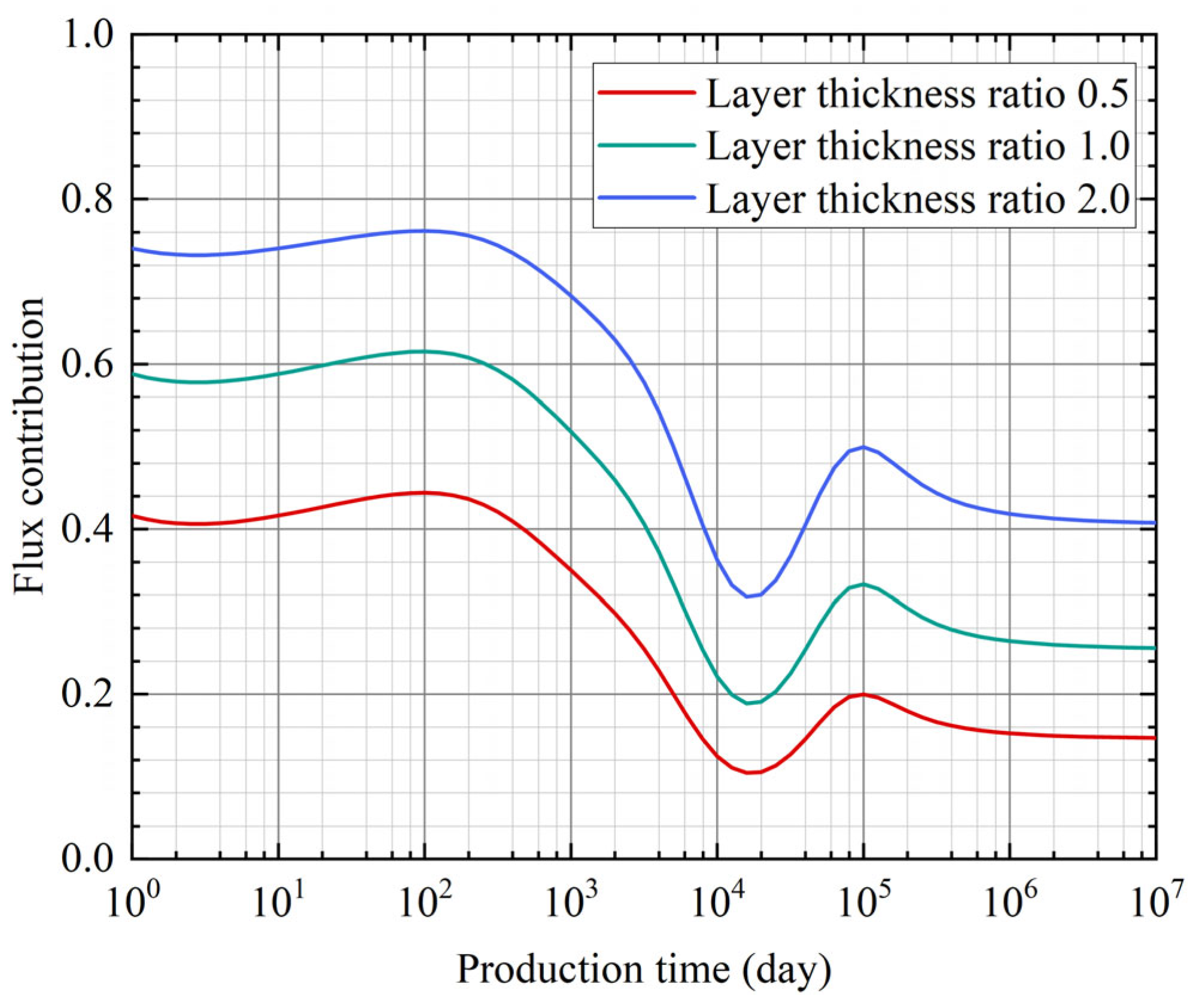
3.3. Layer Thickness Ratio

Reservoir thickness is directly related to the volume of hydrocarbons present in a reservoir. Different layer thickness ratios are investigated to discuss their influence on the transient rate behavior of multi-superimposed reservoirs, including 0.5, 1, and 1.5. The layer thickness ratio is defined as the ratio of the thickness of a tight gas layer to that of a coalbed methane layer. Figure 8 shows the effect of different layer thickness ratios on the Blasingame decline type curve. With the increase in the layer thickness ratio, all three types of curves gradually increase throughout the production period. A higher layer thickness contains a larger volume of recoverable reserve, leading to higher production rates over the life of the well. Figure 9 shows the effect of different layer thickness ratios on the flux contribution of the tight gas layer. Compared with Figure 4 and Figure 7, one can find that the formation thickness has a significant effect on the increase in the flux contribution throughout the production period. The reason is that the gas reserves in different regions will be exploited successively in the whole production. With the increase in reservoir thickness, the recoverable reserves in all regions have increased. This results in significantly higher output in each production period than before. Moreover, the study of Zhao et al. [14] highlights that the layer thickness ratio significantly affects the overall production potential. When the coalbed methane layer is thinner than the tight gas layer, the initial production rate is largely driven by tight gas. However, as production progresses, the thinner coalbed methane layer can still contribute considerably, ensuring a more prolonged and stable output in the late production, which aligns with our findings. It is worth noting that, in cases where the coalbed methane layer is significantly thicker than the tight gas layer, their study suggests that single-layer production may be more advantageous than co-production.

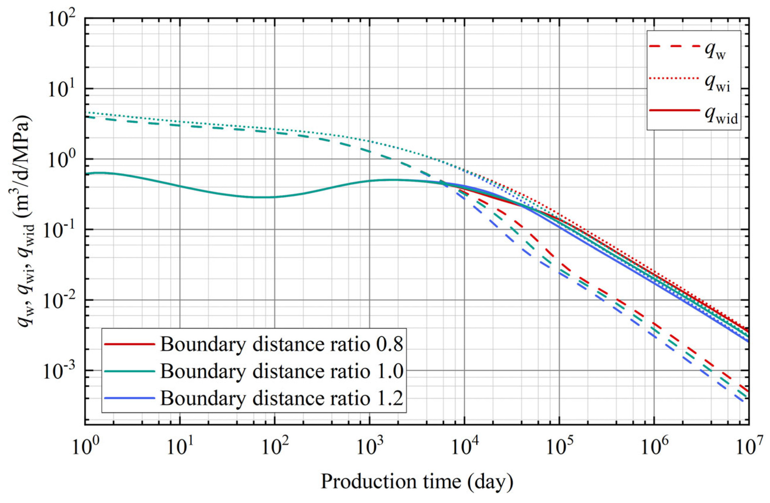
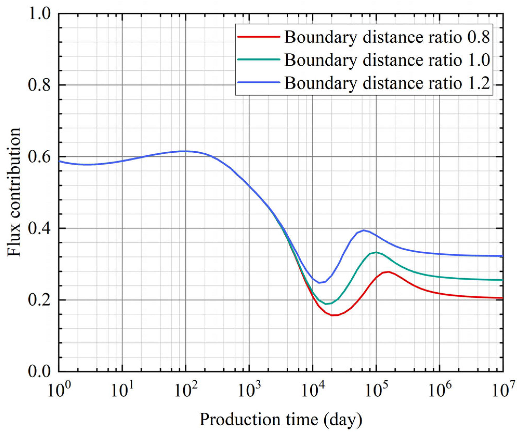
3.4. Boundary Distance Ratio

In this section, the boundary distance refers to the distance from the production well to the boundary of region 2. To understand the effect of boundary distance on gas production, three boundary distance ratios (i.e., 0.8, 1, and 1.2) are discussed. The boundary distance ratio is defined as the ratio of the boundary distance of a tight gas layer to that of a coalbed methane layer. Figure 10 shows the effect of different boundary distance ratios on the Blasingame decline type curve. As can be seen from the figure, the reservoir entered the boundary dominant flow pattern earlier under a smaller boundary distance ratio. This is because the smaller the boundary distance, the shorter the time for the pressure to reach the boundary [27,28]. In addition, with a smaller boundary distance, the well stays in the transient flow regime for a shorter period. This is reflected in the Blasingame decline curve as a quicker decline in production rate. Figure 11 shows the effect of different boundary distance ratios on the flux contribution of the tight gas layer. Since the production well is primarily influenced by the flow in the near-well region, the boundary effect’s contribution to flux is delayed. Thus, with an increased boundary distance, the flux contribution of the tight gas layer exhibits a significant rise in the late production, while having little effect in the early production.

4. Conclusions

In this work, the authors propose an analytical model for a multi-superimposed coal-measure reservoir based on a five-linear flow model. With the aid of the proposed model, the effect of several parameters on the transient rate behavior is investigated. By analyzing the Blasingame decline curve and layered flux contribution, we can draw the following conclusions:

• The influence of different fracture conductivity ratios on the Blasingame decline curve and layer-specific flux contribution is particularly noticeable during the early and middle stages of production. A larger fracture conductivity reduces flow resistance, resulting in a reduced pressure drop and increased cumulative production.
• Longer fractures significantly increase the reservoir contact area, which directly boosts gas production and slows the rate of decline. This effect is especially pronounced in the middle and late production stages of the tight gas layer, where an increased fracture length helps maintain flux contribution as reservoir pressure drops.
• Layer thickness ratios significantly impact production and flux contribution. Increasing thickness boosts recoverable reserves and extends high-production phases.
• A smaller boundary distance leads to earlier boundary flow and a quicker production decline. As the boundary distance increases, higher flux contributions can be observed in the late production.

While the results offer valuable insights into production dynamics, applying them to industrial conditions requires considering factors like geological heterogeneity, operational constraints, and economic feasibility. However, these findings can guide hydraulic fracturing designs and co-production strategies, potentially improving gas recovery and efficiency in some cases.

References

- Zou, C.; Yang, Z.; Huang, S.; Ma, F.; Sun, Q.; Li, F.; Pan, S.; Tian, W. Resource types, formation, distribution and prospects of coal-measure gas. Pet. Explor. Dev. 2019, 46, 451–462. [Google Scholar] [CrossRef]
- Li, Y.; Zhou, D.; Wang, W.; Jiang, T.; Xue, Z. Development of unconventional gas and technologies adopted in China. Energy Geosci. 2020, 1, 55–68. [Google Scholar] [CrossRef]
- Liang, W.; Wang, J.; Li, P. Gas production analysis for hydrate sediment with compound morphology by a new dynamic permeability model. Appl. Energy 2022, 322, 119434. [Google Scholar] [CrossRef]
- Mastalerz, M.; Drobniak, A. Coalbed methane: Reserves, production, and future outlook. In Future Energy; Elsevier: Amsterdam, The Netherlands, 2020; pp. 97–109. [Google Scholar] [CrossRef]
- Li, L.; Ma, S.; Liu, X.; Liu, J.; Lu, Y.; Zhao, P.; Kassabi, N.; Hamdi, E.; Elsworth, D. Coal measure gas resources matter in China: Review, challenges, and perspective. Phys. Fluids 2024, 36, 071301. [Google Scholar] [CrossRef]
- As, D.V.; Bottomley, W.; Furniss, J.P. The characterisation of differential depletion in a thinly layered coal seam gas reservoir using packer inflation bleed off tests PIBOTs. In Proceedings of the SPE Asia Pacific Oil and Gas Conference and Exhibition, SPE, Jakarta, Indonesia, 17–19 October 2017; p. D011S006R003. [Google Scholar] [CrossRef]
- Tao, S.; Chen, S.; Pan, Z. Current status, challenges, and policy suggestions for coalbed methane industry development in China: A review. Energy Sci. Eng. 2019, 7, 1059–1074. [Google Scholar] [CrossRef]
- Qin, Y.; Shen, J.; Shen, Y. Joint mining compatibility of superposed gas-bearing systems: A general geological problem for extraction of three natural gases and deep CBM in coal series. J. China Coal Soc. 2016, 41, 14–23. [Google Scholar] [CrossRef]
- Wu, Y.; Pan, Z.; Zhang, D.; Lu, Z.; Connell, L.D. Evaluation of gas production from multiple coal seams: A simulation study and economics. Int. J. Min. Sci. Technol. 2018, 28, 359–371. [Google Scholar] [CrossRef]
- Wei, Y.; Jia, A.; He, D.; Wang, J.; Han, P.; Jin, Y. Comparative analysis of development characteristics and technologies between shale gas and tight gas in China. Nat. Gas Ind. 2017, 37, 43–52. [Google Scholar] [CrossRef]
- Zhang, L.; Shan, B.; Zhao, Y. Production performance laws of vertical wells by volume fracturing in CBM gas reservoirs. Nat. Gas Ind. 2017, 37, 38–45. [Google Scholar] [CrossRef]
- Wang, S.; Gao, W.; Guo, T.; Bao, S.; Jin, J.; Xu, Q. The discovery of shale gas, coalbed gas and tight sandstone gas in Permian Longtan formation, Northern Guizhou Province. Geol. China 2020, 47, 249–250. [Google Scholar] [CrossRef]
- Huang, S.; Kang, B.; Cheng, L.; Zhou, W.; Chang, S. Quantitative characterization of interlayer interference and productivity prediction of directional wells in the multilayer commingled production of ordinary offshore heavy oil reservoirs. Pet. Explor. Dev. 2015, 42, 533–540. [Google Scholar] [CrossRef]
- Zhao, S.; Wang, Y.; Li, Y.; Wu, X.; Hu, Y.; Ni, X.; Liu, D. Co-production of tight gas and coalbed methane from single wellbore: A simulation study from northeastern Ordos Basin, China. Nat. Resour. Res. 2021, 30, 1597–1612. [Google Scholar] [CrossRef]
- Hamawand, I.; Yusaf, T.; Hamawand, S.G. Coal seam gas and associated water: A review paper. Renew. Sustain. Energy Rev. 2013, 22, 550–560. [Google Scholar] [CrossRef]
- Sang, S.; Zheng, S.; Yi, T.; Zhao, F.; Han, S.; Jia, J.; Zhou, X. Coal measures superimposed gas reservoir and its exploration and development technology modes. Coal Geol. Explor. 2022, 50, 3. [Google Scholar] [CrossRef]
- Ou, C.H.; Li, C.C.; He, J. Comprehensive evaluation of gas zone in multi-layer sandstone gas reservoir. Adv. Mater. Res. 2014, 1056, 80–83. [Google Scholar] [CrossRef]
- Guo, J.; Meng, F.; Jia, A.; Dong, S.; Yan, H.; Zhang, H.; Tong, G. Production behavior evaluation on multilayer commingled stress-sensitive carbonate gas reservoir. Energy Explor. Exploit. 2021, 39, 86–107. [Google Scholar] [CrossRef]
- Zhong, G.; Li, S.; Tang, D.; Tian, W.; Lin, W.; Feng, P. Study on Co-production compatibility evaluation method of multilayer tight gas reservoir. J. Nat. Gas Sci. Eng. 2022, 108, 104840. [Google Scholar] [CrossRef]
- Lu, J.; Rahman, M.; Yang, E.; Alhamami, M.; Zhong, H. Pressure transient behavior in a multilayer reservoir with formation crossflow. J. Pet. Sci. Eng. 2022, 208, 109376. [Google Scholar] [CrossRef]
- Zhang, T.; Wang, B.; Zhao, Y.; Zhang, L.; Qiao, X.; Zhang, L.; Qiao, X.; Zhang, L.; Guo, J.; Thanh, H. Inter-layer interference for multi-layered tight gas reservoir in the absence and presence of movable water. Pet. Sci. 2024, 21, 1751–1764. [Google Scholar] [CrossRef]
- Huang, L.; Wang, X. Controlling factors towards co-production performance of coalbed methane and tight sandstone gas reservoirs. Arab. J. Geosci. 2021, 14, 2344. [Google Scholar] [CrossRef]
- Bumb, A.C.; McKee, C.R. Gas-well testing in the presence of desorption for coalbed methane and devonian shale. SPE Form. Eval. 1988, 3, 179–185. [Google Scholar] [CrossRef]
- Huang, S.; Yao, Y.; Ma, R.; Wang, J. Analytical model for pressure and rate analysis of multi-fractured horizontal wells in tight gas reservoirs. J. Pet. Explor. Prod. Technol. 2019, 9, 383–396. [Google Scholar] [CrossRef]
- Stalgorova, E.; Mattar, L. Analytical model for history matching and forecasting production in multifrac composite systems. In Proceedings of the SPE Canada Unconventional Resources Conference, SPE, Calgary, AB, Canada, 30 October–1 November 2012; p. SPE-162516. [Google Scholar] [CrossRef]
- Stehfest, H. Algorithm 368: Numerical inversion of Laplace transforms [D5]. Commun. ACM 1970, 13, 47–49. [Google Scholar] [CrossRef]
- Zhao, Y.L.; Xie, S.C.; Peng, X.L.; Zhang, L.H. Transient pressure response of fractured horizontal wells in tight gas reservoirs with arbitrary shapes by the boundary element method. Environ. Earth Sci. 2016, 75, 1220. [Google Scholar] [CrossRef]
- Wei, M.Q.; Duan, Y.G.; Chen, W.; Fang, Q.T.; Li, Z.L.; Guo, X.R. Blasingame production decline type curves for analysing a multi-fractured horizontal well in tight gas reservoirs. J. Cent. South Univ. 2017, 24, 394–401. [Google Scholar] [CrossRef]