Abstract
In light of Switzerland’s 2050 energy goals, the nation aims to boost its domestic hydroelectric output, notably focusing on small-scale hydroelectric power plants. Concurrently, there is an effort to renovate hydroelectric plants to make them more environmentally friendly, emphasizing ecological flow regulation to improve river conditions. This study explores the application of a non-proportional flow allocation method to better assess both ecological and economic outcomes. Unlike traditional fixed or proportional flow methods, this approach allows for a more dynamic balance between hydropower generation and riverine ecosystem health. This study focuses on two key species, brown trout and grayling. In particular, this work highlighted that trout are better suited for low-flow conditions (Weighted Usable Area, WUA, peaks below 1 m3/s), while grayling require significantly higher flows (WUA peaks over 4.5 m3/s). This disparity in habitat preferences raises concerns about the current reliance on single-species models, emphasizing the need for multi-species ecological assessment in future studies. When applied to a small hydropower plant in the Swiss Jura, the non-proportional flow method resulted in an improvement of ecological conditions of at least 37.7%, which consequently led to a reduction of the hydroelectric production of at least 10%. Through strategic upgrades to the facility (e.g., by minimizing hydraulic losses, implementing more efficient turbines, or incorporating photovoltaic panels over water channels), it is possible to simultaneously enhance both energy output and environmental sustainability. These findings suggest that non-proportional flow allocation holds significant potential for broader use in sustainable hydropower management, providing a pathway toward meeting both energy production and ecological conservation goals.
1. Introduction
In Switzerland, hydroelectric power plants generate the largest share of domestic electricity, accounting for 39,500 GWh in 2021, which represents 61.5% of the total production. Additionally, small-scale hydropower plants contribute 4100 GWh annually, which is slightly over 6% of the total electricity production of the country [1]. As Switzerland aims for carbon neutrality by 2050, enhancing hydroelectric production will be crucial in achieving this goal [2]. While large power plants will undoubtedly be pivotal for the carbon neutrality aspirations of the country, given their potential to increase production by anywhere from 210 GWh/year to 2000 GWh/year, small-scale hydropower plants can also be of interest in this regard.
Switzerland relies on hydroelectric power plants for its 2050 energy strategy, but this approach clashes with the goal of ensuring high ecological quality for its waterways. Watercourses with dynamic hydrological regimes and bedloads are vital for biodiversity and ecosystem services [3]. Dams harm ecosystems by disrupting downstream flows, reducing flooded areas, altering species composition, and increasing clogging by fine sediment [4]. To address these problems, the Swiss Water Protection Act enforced by the Federal Office for the Environment (FOEN) mandates that all hydropower plants ensure a minimum ecological, or residual, flow in the watercourses they exploit. This residual flow is defined as the minimal quantity of water necessary to maintain fundamental ecosystem functions, habitat quality, groundwater interactions, and pollutant degradation. This requirement aligns with Article 31 of the Water Protection Ordinance (OEAux) [5,6].
The conflict between hydropower production and the ecological quality of Swiss watercourses is well documented in the “Energieeinbussen aus Restwasserbestimmungen—Stand und Ausblick” 2018 report from the “Schweizerischer Wasserwirtschaftsverband” [7]. It highlights that stringent ecological standards are incompatible with Switzerland’s 2050 energy strategy. Even in an optimal scenario, projections from 2018 to 2050 anticipate an annual electricity reduction of 2280 GWh. Therefore, finding a balance between environmental preservation and hydropower development presents a significant challenge for Switzerland’s energy future.
In Switzerland, the current practice involves maintaining a constant minimum residual flow seasonally or throughout the year. However, in the past decade, there has been research aimed at improving flow distribution by exploring a non-proportional allocation approach [8,9]. More recently, Razurel et al. (2016) [10] suggested a non-proportional flow distribution method based on the Fermi function. This approach offers operating conditions close to the Pareto frontier, improving ecological and economic aspects more effectively than traditional flow management policies. Furthermore, this approach has the potential to reconcile ecological imperatives with Switzerland’s 2050 energy strategy, thus mitigating the conflict between hydropower production and river ecology. Specifically, these studies have demonstrated that river ecology and hydroelectric production exhibit a non-linear relationship, indicating that even small changes in river discharge allocation can lead to significant improvements in environmental quality. This makes non-proportional distribution methods highly promising for future management practices.
This study is structured in two key phases. The first focuses on quantitatively assessing the habitats of brown trout (Salmo trutta) and grayling (Thymallus thymallus) populations to provide a more comprehensive understanding of their health status in the study area. The second aims to investigate the flow allocation management of a small hydroelectric scheme in the Swiss Jura region. In this study, a method is proposed to evaluate the impacts of various ecological flows on both the electricity produced by the hydropower plant and the habitat available to native river brown trout (Salmo trutta L.). This will be accomplished by implementing the method developed by Razurel et al. (2016) [10] and employing their numerical model as detailed in their 2018 study [11]. Furthermore, the approach used in this study acts as an improvement of the single-species one suggested by Rauzel et al. (2016) [10]. It considers the ecology of both brown trout and grayling together, even if the second species is not directly included in the model [10].
The goal of this work is to take a first preliminary step in developing a methodology able to combine economic assessment and trout ecology. The proposed approach applies Razurel’s methodology to a real-world hydroelectric power plant context, analyzing both ecological and economic outcomes [10]. The secondary and more general purpose of this study is to gain more understanding of the method’s application while laying the foundation for future improvements and broader applications, such as the use of a multi-species approach.
2. Study Area Status
2.1. The Hydrology
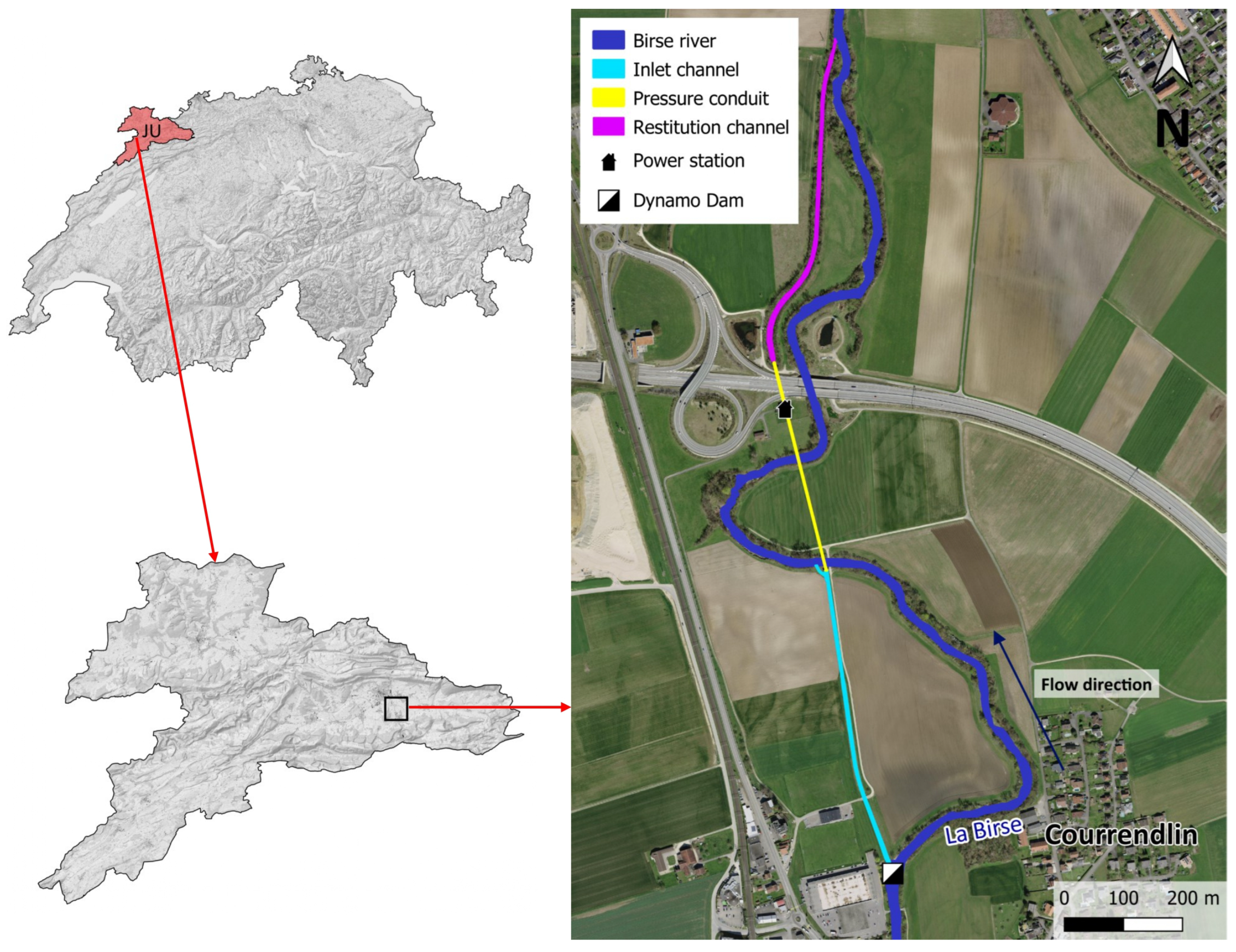
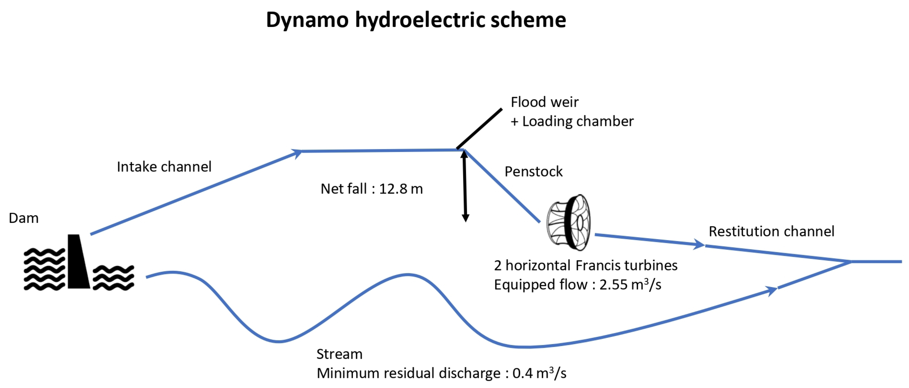
This research focuses on the Dynamo hydroelectric scheme, located along the Birse river in Courrendlin (Figure 1). The catchment area has a “jurassien” pluvio-nival regime type, although recent data shows a disappearance of the spring peak discharge due to climate change inducing less snow accumulation in winter [12].

Figure 1.
Map showing the location and the different parts of the Dynamo hydroelectric scheme.
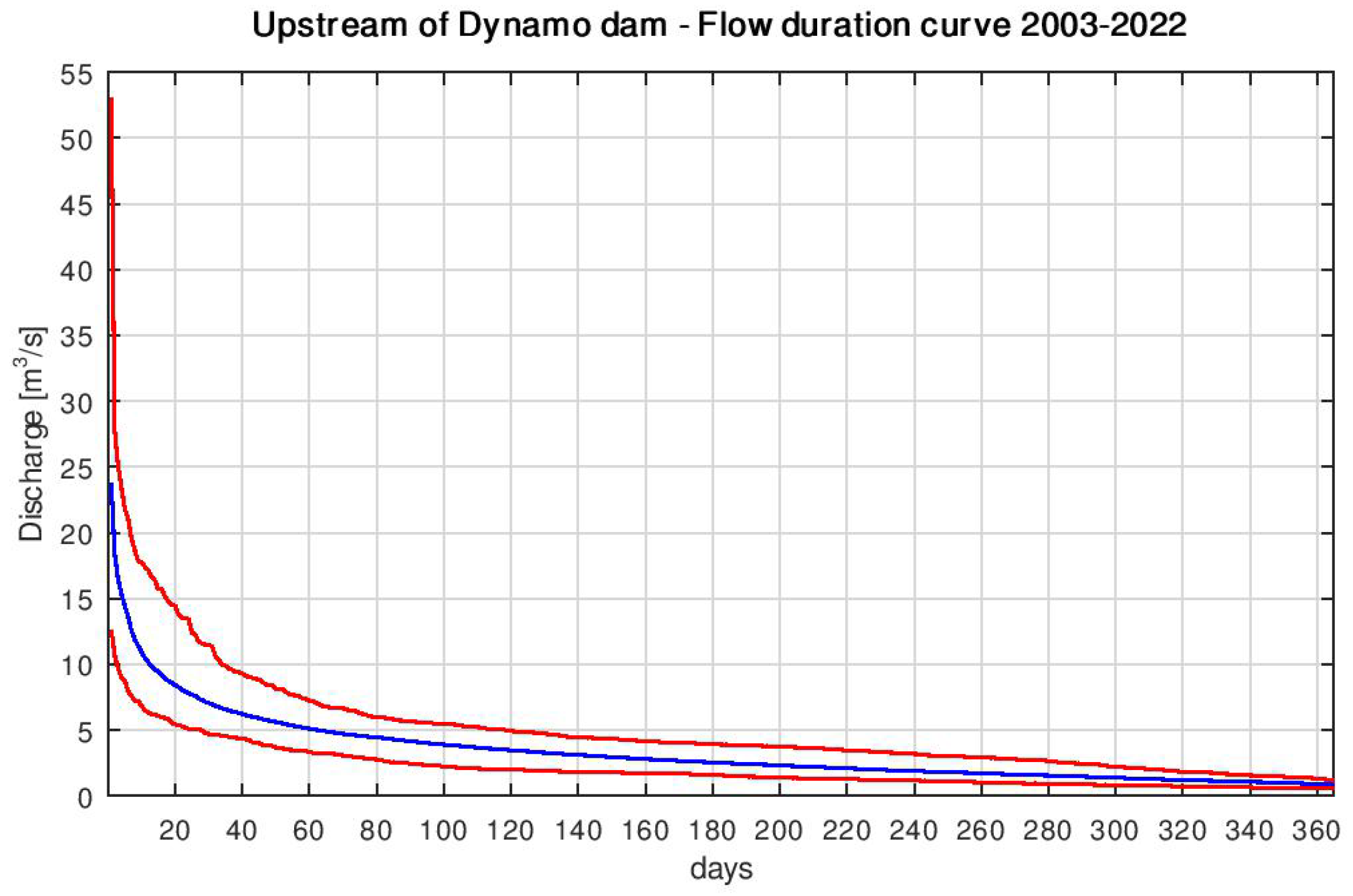
Analyses of daily flow data from the past two decades (2003–2022) show that the average discharge, , is 1.03 m3/s. The flow duration curve (Figure 2) for this period presents a flow discharge above 5 m3/s for less than 60 days per year.
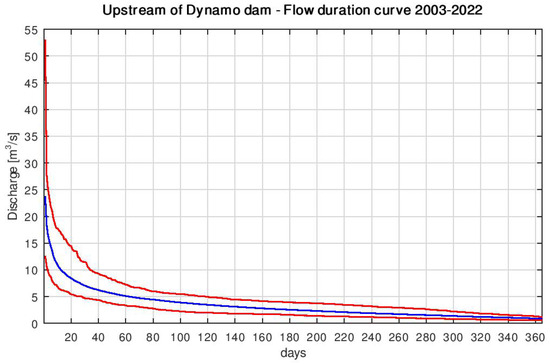
Figure 2.
Flow duration curve for flows upstream of the Dynamo hydroelectric dam in the period 2003–2022. The blue line is the average curve, while the red lines are the minimum and maximum values.
According to Article 3, Letter (a) of Decree No. 53G67, which governs the transfer and renewal of hydraulic concession, dated 15 March 2005, the ecological flow of the Dynamo plant is stipulated at 0.4 m3/s (rounded), with a calculated value of 0.412 m3/s [13]. The inflow time series to the dam are estimated using data from hydrological station No. 2122, known as “La Charrue”, located in Moutier, approximately 8.5 km upstream. This estimation involves weighting the data by the ratio of the respective catchment areas. The analysis is based on daily flow recorded over the last twenty years (2003–2022).
2.2. Fish Population Ecology
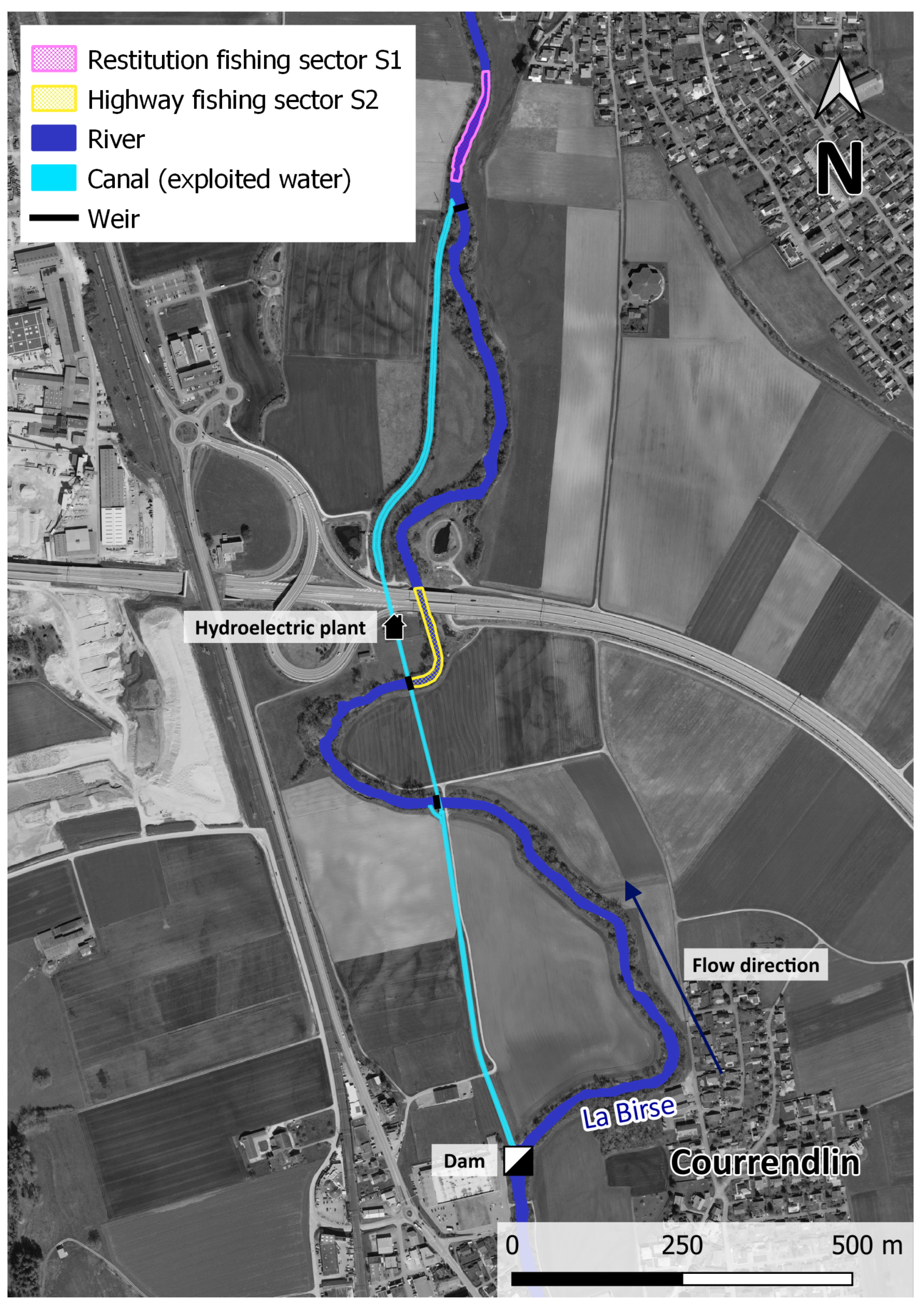
On 12 July 2023, the Jura Environmental Office (ENV) conducted an electrofishing survey in the study area to assess the impacts of the hydropower plant on the river reach. Two different sections were sampled, one downstream of the restitution junction, which is not affected by the water withdrawals necessary to operate the Dynamo (sector S1, length 154 m, pink area in Figure 3), and the other upstream of the restitution junction, which is directly affected by the Dynamo operation (sector S2, length 152 m, yellow area in Figure 3).
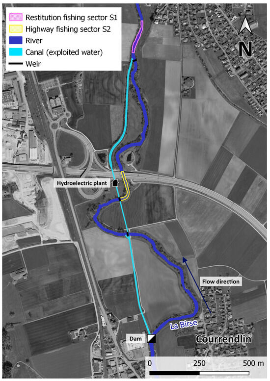
Figure 3.
The locations of the surveyed reach S1 and S2 by electrofishing on 12 July 2023.
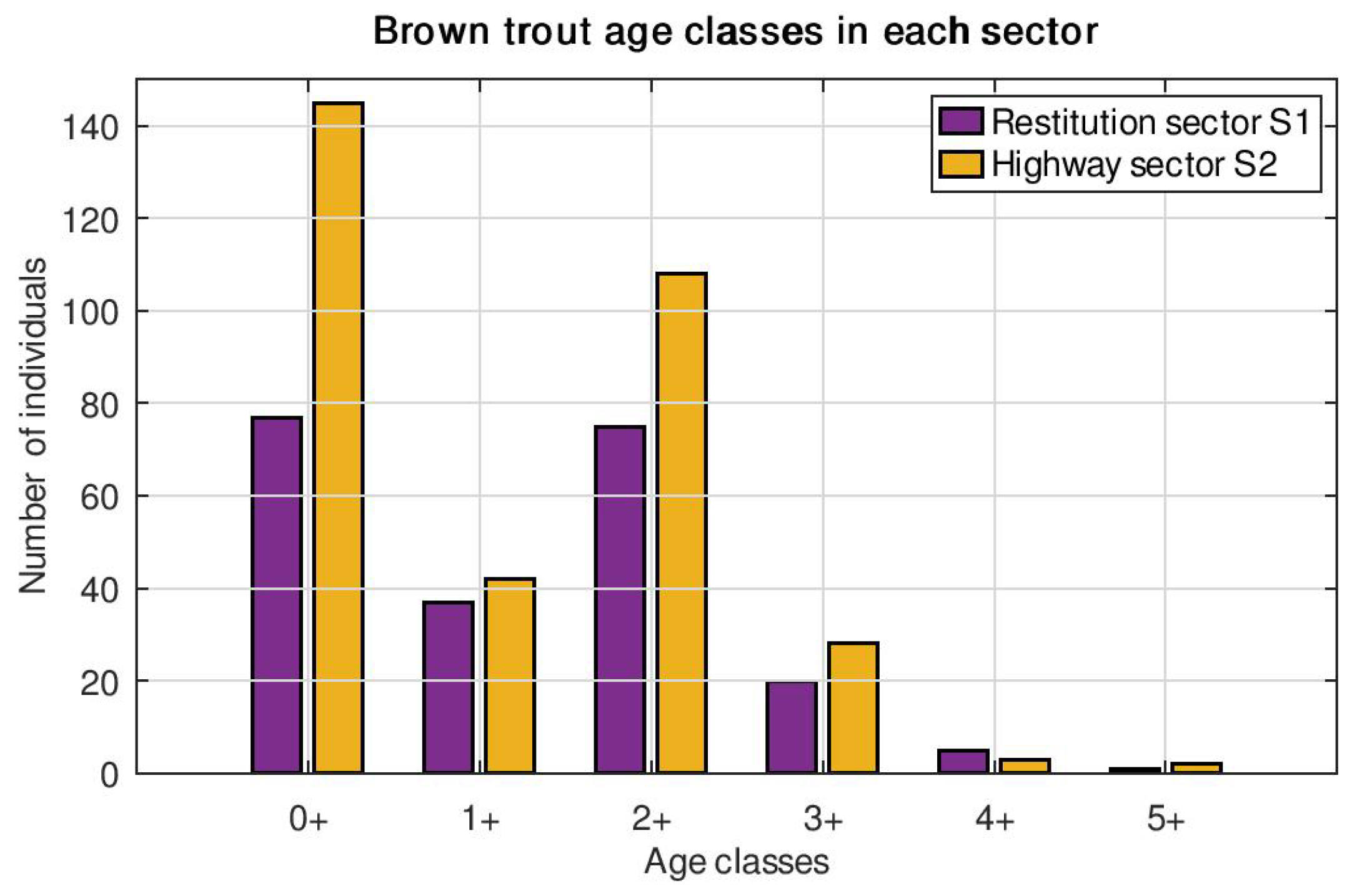
Data on five different species were collected during the electrofishing carried out by the Jura canton (Table 1). In sector S1 (downstream of the restitution), fish diversity was slightly higher than in sector S2, with five species recorded, compared with the four species found in sector 2. The most common species were brown trout (Salmo trutta fario) and sculpin (Cottus gobio). Grayling (Thymallus thymallus) were more abundant in S1 than in S2. Barbel (Barbus barbus) were counted in both sectors, but only two individuals were counted in S1, compared with 18 in S2. Minnows (Phoxinus phoxinus) were counted only in sector S1, with only three individuals. Between the two target species for this study (trout and grayling), trout clearly predominated in sector S2, subject to ecological flow, with 328 individuals compared with only 10 grayling (see Table 1). This disparity diminished in sector S1, where the difference was reduced to 215 trout versus 43 grayling.

Table 1.
Number of individuals collected for each species in the two sectors.
The number of individuals per age class for trout and grayling in each sector (Figure 4 and Figure 5) suggests that both species utilize the portion of the Birse not affected by hydropower operations throughout their entire lifespan. On the other hand, while trout of all age classes were present, in sector S2, only 0+ graylings were captured. This suggests that flow modifications caused by the hydropower plant affect grayling distribution.

Figure 4.
Number of trout individuals per each age class in the two sampled sectors. The age classes 0+ to 5+ represent individuals from the 1st to the 6th year of life.
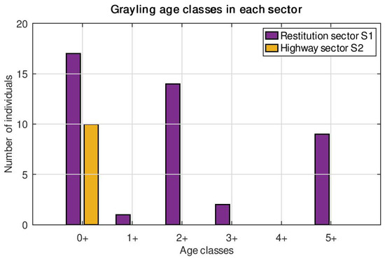
Figure 5.
Number of grayling individuals per each age class in the two sampled sectors. The age classes 0+ to 5+ represent individuals from the 1st to the 6th year of life.
2.3. The Dynamo Hydropower Plant
The hydroelectric power station (hydroelectric scheme, Figure 6) is equipped with two horizontal Francis turbines from Gugler, originally designed with a capacity split of around 2/3:1/3, amounting to 1.70 m3/s and 0.85 m3/s, respectively, resulting in a total equipped discharge capacity of around 2.55 m3/s. The minimum operating flow is set at 0.032 m3/s. The average net head of the Dynamo structure is 12.8 m. The river stretches between the dam and the restitution over a total length of 2.05 km.
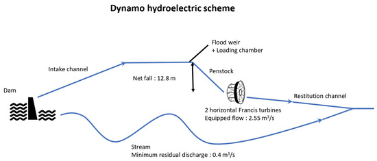
Figure 6.
Schematic drawing of the Dynamo hydroelectric power plant with its main components.
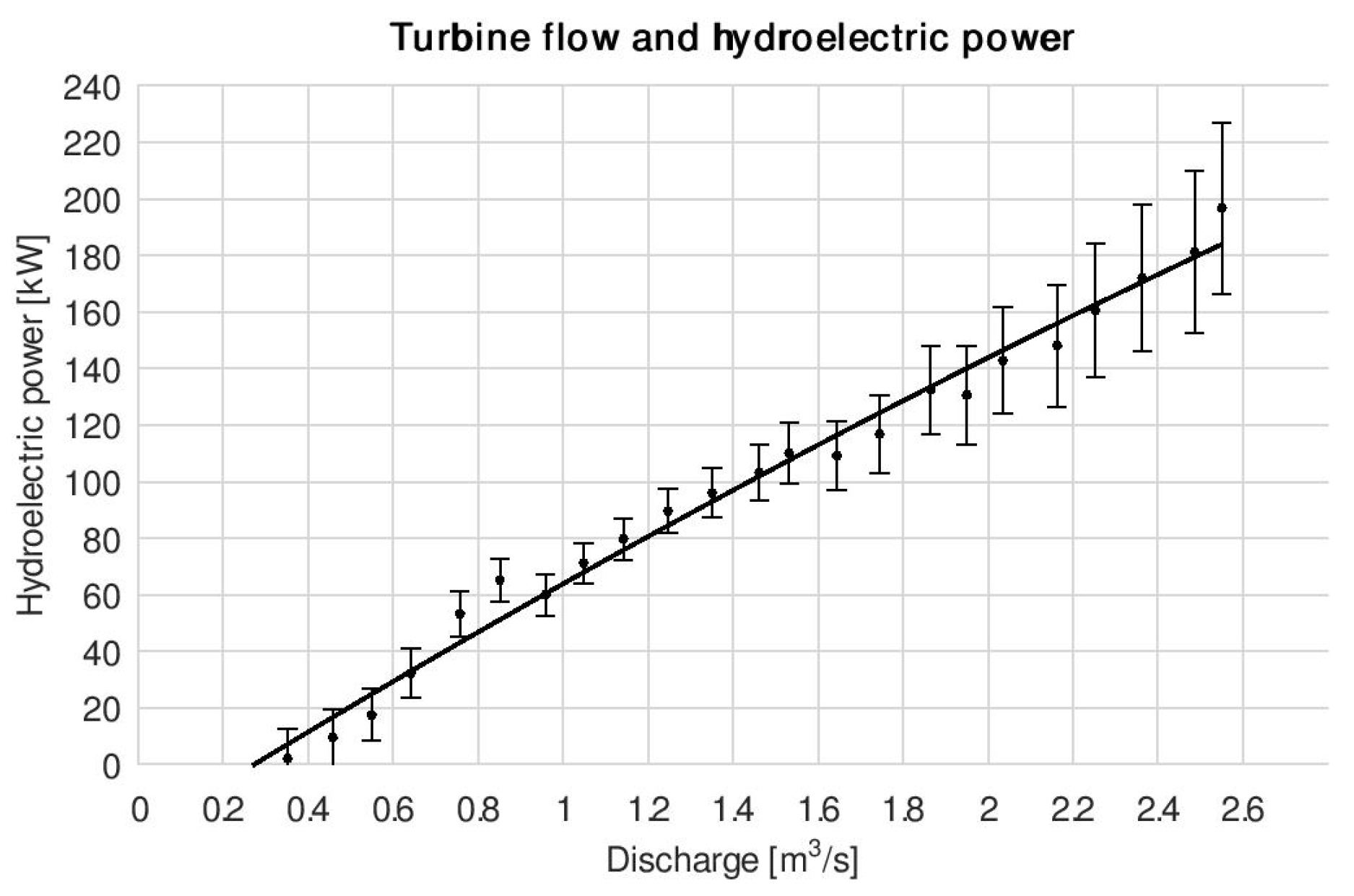
To link energy production with operating flows, hydroelectric production data for 2020–2021 were collected during a visit to the Dynamo power station on 11 May 2023. These production data were correlated to the current operating flow, , using the following formula:
where is the power output of the Dynamo structure at time t, is the overall efficiency of the hydroelectric plant, = 999 kg/m 3 is the density of water (considered constant), g = 9.81 m/s2 is the gravitational acceleration, and = 12.8 m is the average net head. The current operating flow was calibrated from the power output (Equation (1)) and by comparing theoretical and current flows, aiming to validate results and overall consistency. A constant performance was calibrated using Equation (1), testing various efficiencies. values were used along with upstream flows, I, to determine current ecosystem flows, , using the general relation:
Flow adjustments were made while respecting a maximum operating flow of 2.55 m3/s and a minimum ecological flow of 0.4 m3/s. The calibration between the theoretical flow rate and the Dynamo hydroelectric power generation (Figure 7) resulted in an efficiency of the hydropower plant, , of 0.74. The hydroelectric output was compared with the theoretical flow, revealing potential bias, possibly due to data inaccuracies (daily discharges or dysfunctional water intake).
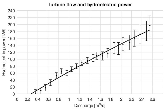
Figure 7.
Relationship between the channel discharge and the Dynamo hydroelectric power generation. The points with the error bars represent the energy production values measured for a corresponding theoretical flow rate, which are deduced from the theoretical flow distribution arriving at the dam. The main line represents the regression curve of the mean values for each rounded discharge.
3. Methodology
3.1. Hydraulic and Habitat Modelling
To quantitatively assess fish habitat, we developed a Habitat Suitability Index (HSI) utilizing a detailed hydraulic model for the study area. This model provided essential parameters such as water velocity and depth, which are crucial for determining habitat suitability for different fish species.
To construct the hydraulic model, we converted elevation data from the SwissSURFACE3D point cloud’s “ground” layer to the Digital Terrain Model (DTM) with a resolution of 0.25 × 0.25 m with the CloudCompare v2.0 software. The SwissSURFACE3D layer is freely available on the website of the Confederation (https://www.swisstopo.admin.ch/fr/modele-altimetrique-swisssurface3d) (accessed on 15 April 2023). As LIDAR data are accurate but lack underwater elevation, we conducted bathymetric surveys on 25–26 April and 6 May 2023, using GPS equipment, including Happy Mönch II GNSS and Happy Lausanne RTK tablet, to refine the DTM. These surveys yielded 843 points, with spacing between longitudinal sections ranging from 10 to 25 m and between transverse points from 0.5 to 2 m. The macroroughness of the bed is simplified in this study by correcting the DTM of the bed. The watercourse granulometry analysis was performed using the BASEGRAIN 2.2 program from ETH Zürich, along with photos of the stream bed taken on 1 June 2023 [14,15]. We processed 33 calibrated images of the bed with BASEGRAIN to obtain granulometry curves.
The 2D hydraulic model was created by using BASEMENT 3.1.1, a program developed by ETH Zürich. This process involved defining a study area, creating a mesh, and specifying boundary conditions. Different roughness zones were established, and stream rocks were integrated into the mesh to enhance the accuracy of the hydraulic model by improving stream path dynamics. Hydraulic results were then implemented in the HABBY 0.26 software to calculate the Habitat Suitability Index (HSI), a species-specific indicator used to assess the suitability of a small section of the river (referred to as a hydraulic unit or river element; Bovee 1986) [16]. This index primarily relies on two hydraulic variables: water depth and water velocity, with the option to consider the substrate grain size.
The species under investigation were brown trout and grayling, both of significant importance in the study area, as outlined in the 2014 fish report [17]. The significance of studying these two species comes from their classification as “potentially in danger” and “in danger”, respectively, according to the 2022 Swiss red list [18]. The biological models used in HABBY are based on the studies by Souchon et al. (1989) [19] and Mallet et al. (2000) [20] for brown trout and grayling, respectively. The model by Souchon et al. (1989) [19] is a large microhabitat study on different fish species, including brown trout. By considering water velocity, water depth, and sediment grain size as hydraulic parameters, they build preference curves for each fish species, which are used for HSI calculation in HABBY. Besides, the Mallet et al. model (2000) [20] for grayling does not consider the sediment grain size but focuses solely on water velocity and depth to compute the HSI. This second model was chosen because the Ain River analyzed in that study is geographically close and similar in characteristics (e.g., medium size, slope) to the Birse River. As the final step, the HSI was used to compute the Weighted Usable Area (WUA) [m2], which is the total area of the river reach that is suitable for the specific fish species. It was obtained by weighting the total wetted area of the river, Awet [m2], with the overall HSI (Nestler et al., 2019) [21] by means of the following formula:
3.2. Ecohydrological and Economic Assessment
Due to its small storage capacity, the storage system of the Dynamo dam has been neglected. As a result, the flow allocation system has been simplified into the same expression as Equation (2). The flow allocation method used in this work to maximize environmental and economic benefit was developed by Gorla and Perona (2018) [11]. This approach integrates hydrological, environmental, and hydroelectric data to construct a non-proportional flow distribution and build a Pareto frontier. The non-proportional flow distribution used in our study was developed by Razurel et al. (2016) (the method is briefly described hereafter; for more details, refer to [10]).
This method is based on an adaptation of the Fermi distribution function, (Equation (4)), which makes it possible to determine the fraction of water redistributed to the ecosystem as follows:
where
In this equation, x is the dimensionless flow rate. The values of a, b, i, and j are the adjustable parameters governing the flow distribution. Parameters a, b have a direct influence on the shape of the curve, inducing a non-proportional flow allocation between and , while c fixes the curve’s arriving point when . In this study, c is fixed at 1. Parameters i and j vary between 0 and 1, the first representing the fraction of water left for the ecosystem when the upstream flow , which corresponds to the start of the competition between ecological and economic indices, while the second represents the fraction of water left for the ecosystem when the upstream flow (i.e., to the end of the competition). In particular,
where is the minimum ecological flow, is the minimum operating flow of the turbine, and is the power plant flow. When the upstream flow is greater than , the water in excess is released back into the river for the ecosystem. Finally, can be expressed with the function as follows:
Additionally, the study by Razurel et al. (2016) [10] suggests that the ecological assessment relative to each flow allocation can be carried out by constructing a global environmental indicator, also called the ecohydrological indicator, Eco. They obtained this indicator by combining Indicators of Hydrologic Alteration (IHA) with habitat suitability parameters for trout derived from WUA curves. In order to simplify the work, graylings have not been included in the model. Adding them to the weighting of habitat suitability would probably make it possible to refine the Eco parameter.
Richter et al. (1996) [22] established 32 IHAs that can provide a robust framework for quantifying the variability in dynamics and deviation between natural and altered flow regimes. The IHAs are divided into five groups, statistically characterizing the annual hydrological variations (e.g., Group 1 the magnitude of monthy water conditions, Group 3 the timing of annual extreme water conditions).
As detailed in Gorla and Perona (2013) [9], we used the IHA to calculate the Rate of non-Attainment, , which identifies the part of the days for which the IHA deviates outside plus/minus one standard deviation, and the coefficient of variation, , which is the ratio between the standard deviation and the mean. Then, for each IHA indicator, k, the hydrological sub-indicators, and , which represent the root mean square distances between the simulated and natural and , are calculated [23] (see Gorla and Perona (2013) [9] for more details):
The fish habitat indicator is derived from the critical thresholds of the WUA curves for brown trout in the juvenile and adult stages. Additionally, following the Continuous Under Threshold (CUT) method proposed by Capra et al. (1995) [24], which consists of identifying and integrating periods when water flow falls below a critical threshold necessary for trout survival, the fish habitat indicators and are calculated. These indices represent the maximum number of consecutive days in which the river flow is below the critical WUA threshold:
Afterwards, the hydrological indicators and the fish habitat indicators are converted into four sub-indicators, , limited between 0 and 1:
where and are the hydrological alteration sub-indicators, and and are the habitat availability sub-indicators. For the hydrological indicators, the subscripts and correspond to the scenarios with the lowest and highest impact on the river, which are the natural flow regime and the minimal flow requirement, respectively. As a final step of this method, it is possible to compute the dimensionless and synthetic ecohydrological indicator, , which gives an ecological score in the sector concerned:
where w is the weight for each indicator (see Gorla et al., 2013 [9] and Razurel et al., 2016 [10] for more details).
This study used a Matlab GUI program (R2015a) to compute the parameters altogether in a single EXE-file, tested and validated in the study of Razurel et al. (2018) [11]. The group AHEAD (Hydro-économie appliquée et dynamique des environnements alpins), based in EPFL Lausanne until 2016 then moved to Edinburgh, created this program to find the optimal water allocation policies at the water intake that maximize the energy production and preserve the riverine ecosystem, using different water allocation functions (i.e., non-proportional, proportional, Minimum Flow Released methods) [10]. This program links energy production and Eco-indicators based on input flows, showing annual energy efficiency relative to Eco-indicators. The Pareto frontier delineates the optimal values for each scenario.
The Matlab model relies on different input data: hourly flow data from 2003 to 2022, hydroelectric production curve, and ecological data. In this case, multiple flow allocation methods were examined. In particular, a constant ecological flow was set at 0.4 m/s, a seasonal approach with a higher ecological flow of 0.6 m/s was used from November to April, a proportional method was used, which suggested having 10–50% of ecological flow allocation based on total flow, and a variable non-proportional method with different parameter combinations was applied to determine the Pareto frontier.
Two design flows were analyzed: the current 2.55 m3/s and a 4 m3/s proposed in the 2012 Dynamo report [13]. The Eco-indicator calculations employed the WUA curves and breakpoints for juvenile and adult trout. Three scenarios were considered for each design flow, giving six scenarios in total. Scenario selection relied on Pareto frontier analysis explained in Section 4.2.
4. Results
4.1. WUA Curves
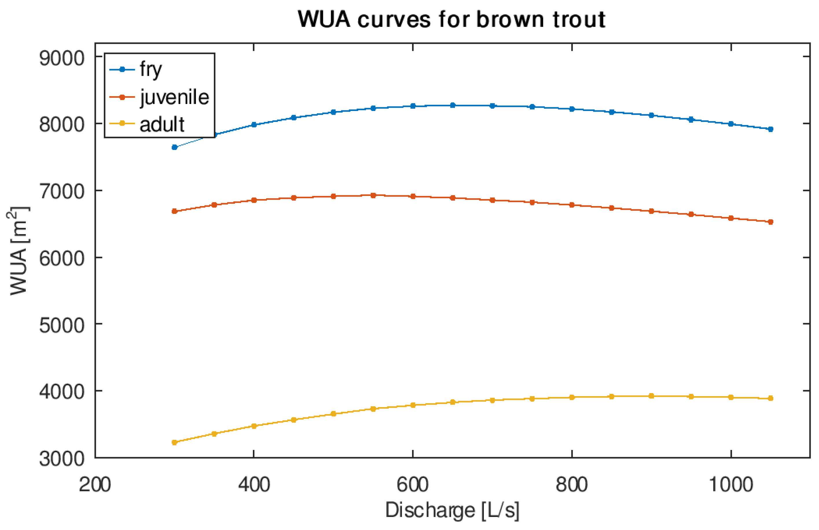
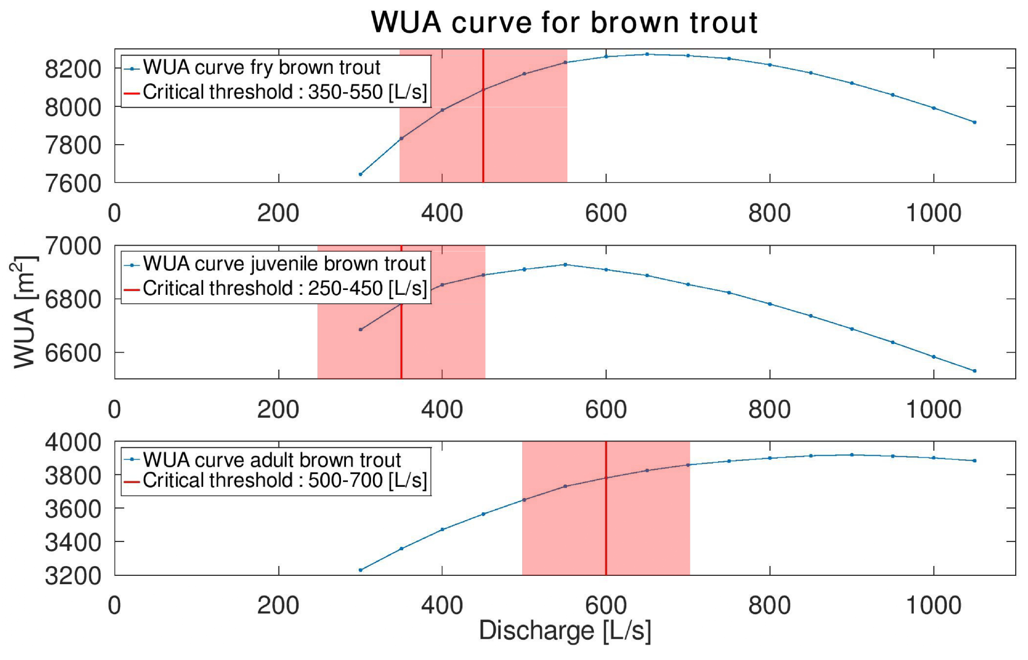
The Weighted Usable Area (WUA) is computed for each design flow to establish the relationship between flow and habitat suitability. These curves (Figure 8 and Figure 9) illustrate three main life stages of brown trout: fry (0+, trout in the first year), juvenile (1+, trout in the second year), and adult (>2+, trout from the third year), across flows ranging from 300 L/s to 1050 L/s. The peak of the WUA curves represents the optimal flow rate for maximizing the surface area of aquatic habitats. Specifically, the maxima of the WUA curves for the three different life stages are 650 L/s, 550 L/s and 900 L/s, accordingly corresponding to WUA values of 8272 m2, 6927 m2, and 3919 m2. The minimum ecological flow is 400 L/s, which corresponds to WUA values of 7980 m2, 6852 m2, and 3472 m2 for fry, juvenile, and adult stages, respectively. A critical threshold is defined on each of the brown trout WUA curves, representing the flow rate at which a significant breakpoint occurs on the curve. These critical thresholds for fry, juvenile, and adult stages are approximately 450 L/s, 350 L/s, and 600 L/s, which correspond to WUA values of 8081 m2, 6790 m2, and 3771 m2, respectively. (See Section 3.2 for the application).

Figure 8.
WUA curves for fry, juvenile, and adult brown trout. The minimum ecological flow is 400 L/s.
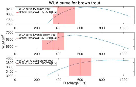
Figure 9.
WUA curves and critical thresholds for fry, juvenile, and adult brown trout. The critical thresholds for these stages are 450 L/s, 350 L/s, and 600 L/s, respectively.
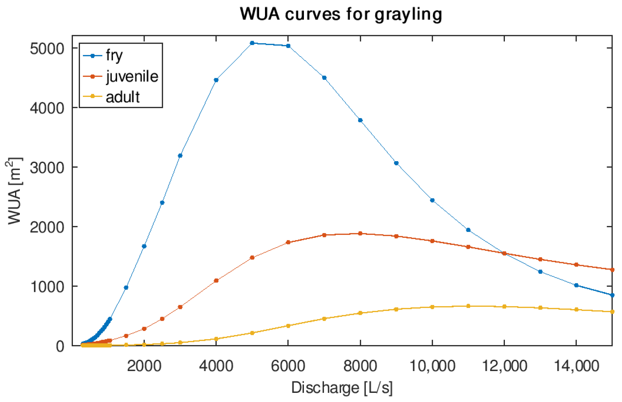
The WUA curves are also computed for grayling (Thymallus thymallus), keeping the same distinction into life stages (Figure 10). In these cases, the flow ranges from 300 L/s to 15,000 L/s. The maxima of these curves are located at a considerably higher flow rate than the ones for brown trout. The WUA curves for grayling follow an exponential progression for all three life stages between 300 and 3000 L/s. This suggests that this species would benefit from increased habitable surface area for increased flow between these values.

Figure 10.
Comparison between the WUA curves for grayling fry, juvenile, and adult stages.
4.2. Ecohydrological and Economic Assessment
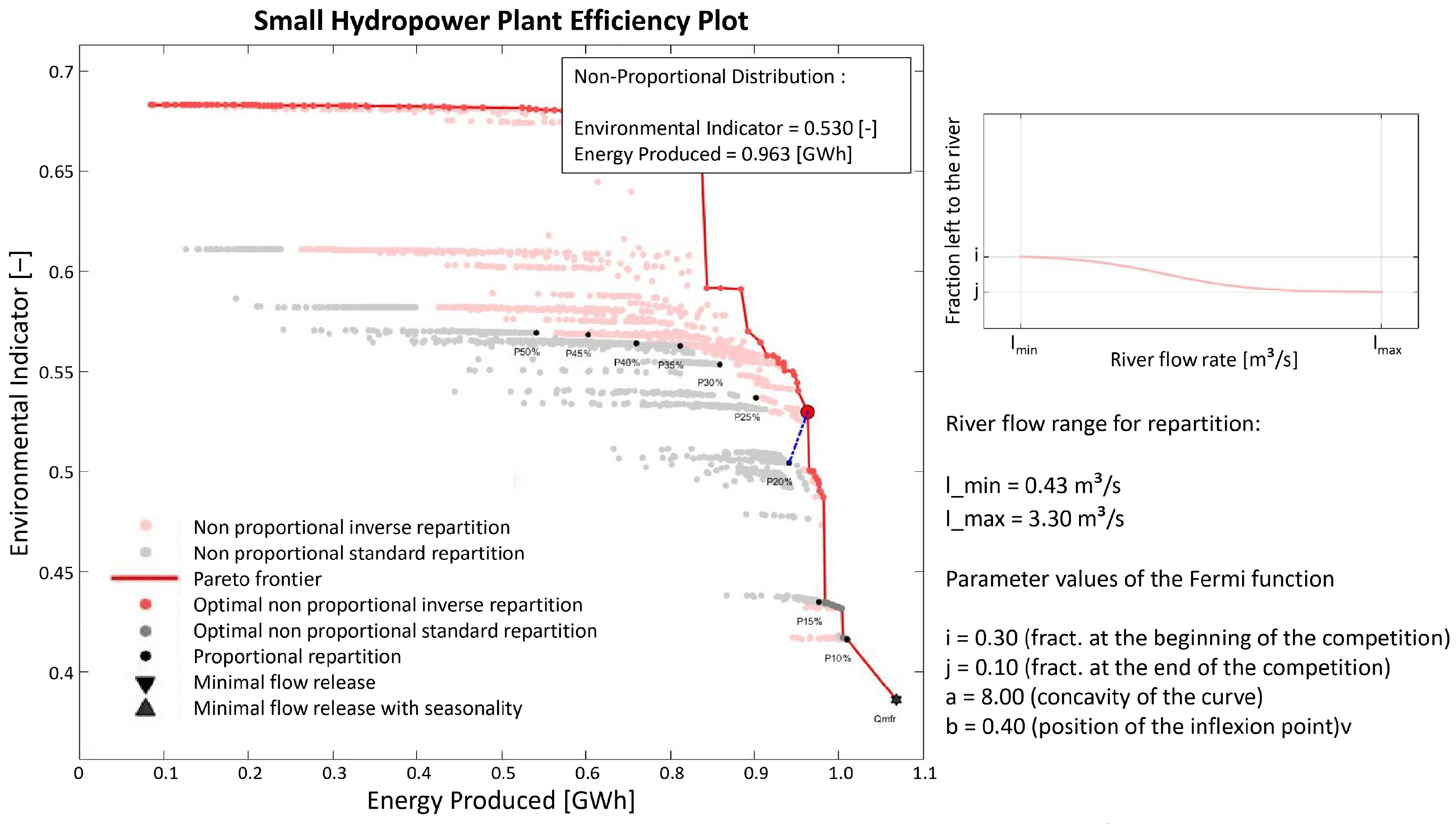
The current situation at the Dynamo power plant, with an equipped flow of 2.55 m3/s (Figure 11), is compared with the projected situation with an equipped flow of 4 m3/s (Figure 12).

Figure 11.
Pareto front analysis between hydroelectric production and the environmental indicator (Eco-index). Results for an equipped flow of 2.55 m3/s. Scenarios with constant ecological flow, both with and without seasonality, are symbolized by black triangles (straight and inverse, respectively). Proportional flow distributions are indicated by black dots. The other dots refer to non-proportional flow distributions. The red line corresponds to the Pareto frontier, where each gray or red point along the line comprises an optimal parameterization of the Fermi function coefficients (a, b, i, j) for a non-proportional flow distribution. The other transparent dots refer to a non-proportional flow distribution with sub-optimal parameterization.
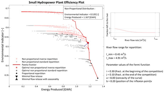
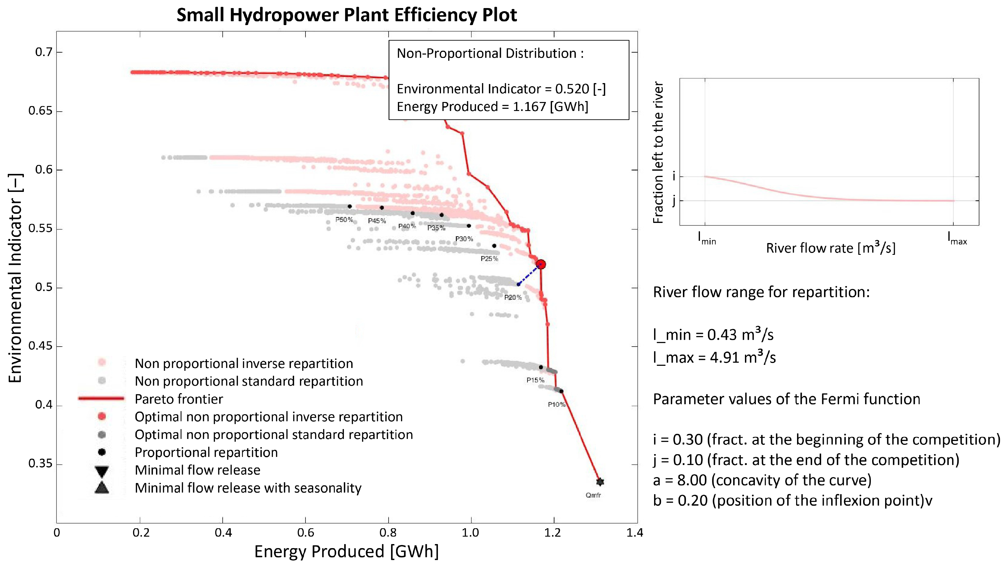
Figure 12.
Pareto front analysis between hydroelectric production and the environmental indicator (Eco-index). Results for an equipped flow of 4 m3/s.
The traditional method of allocating a fixed ecological flow with or without considering seasonality is the most energetically efficient, but the least environmentally friendly. Proportional flow allocation improves environmental impact compared with the fixed ecological flow approach yet it results in a significant loss of hydroelectric production. Finally, non-proportional flow allocation is the best option for balancing environmental needs and hydropower production, as already proven in Razurel et al. (2016) [10]. As proportional flow allocation gives less promising results than non-proportional flow allocation, only non-proportional allocation proposals are considered for choosing scenarios (see Figure 11 and Figure 12).
The trend of the Pareto front curve (Figure 11 and Figure 12) is interesting when the environmental benefit increases drastically (vertical progression of the curve) without involving much loss of hydroelectric production. The points of interest are therefore chosen at the peak of these trends, just before a drop in hydroelectric production (horizontal progression of the curve).
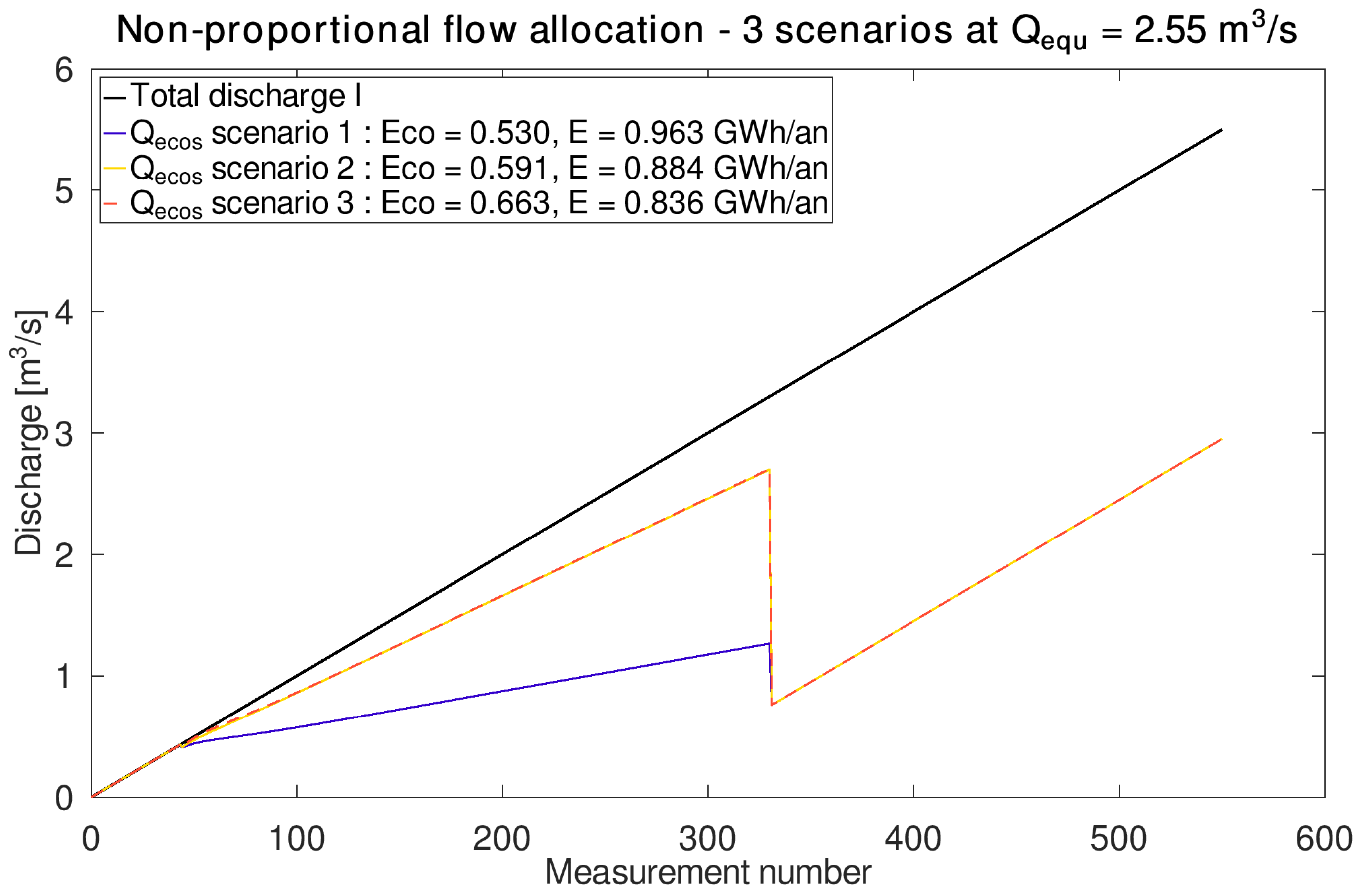
The trend that emerges from this comparison is that an increase in ecological benefit implies a decrease in hydroelectric production. The Fermi function coefficients corresponding to each scenario are summarized in Table 2 along with the results of each scenario, expressed in terms of Eco-indicator and hydroelectric production. These results are further compared with the current flow allocation method, where a constant ecological flow is assumed. Focusing on the current equipped flow of 2.55 m3/s at Dynamo, Scenario 1 presents an economic loss (−10% of produced energy) but an already important environmental benefit (+37.7% of habitat gain). Scenarios 2 and 3 offer increasing environmental advantages, albeit with hydroelectric losses of −17.4% and −21.9%, respectively. However, their similarities pose mechanical adjustment challenges and are vulnerable to uncertainties. Assuming an equipped flow of 4 m3/s at Dynamo, Scenario 4 shows an economic benefit of 9.1%, which is the best among all scenarios. The environmental index improvement of +35.1% is slightly lower than the one in Scenario 1. Scenarios 5 and 6 surpass Scenario 4 in terms of the environmental index but with greater economic losses (+6.2% and −8.8%, respectively).
Table 2.
Summary of the Fermi function coefficients corresponding to each scenario (S). In the table, is the environmental index, E is the hydroelectricity produced, is the current scenario using a fixed ecological flow method and an equipped flow of 2.55 m3/s, is the equipped flow, and the rest are the parameters described in Section 3.2.
Flow Allocation for the Six Scenarios
The flow distributions of Scenarios 1–3 for an equipped flow of 2.55 m3/s are compared withgether (Figure 13), while Scenarios 4–6 are contrasted for an equipped flow of 4 m3/s (Figure 14). The curves obtained, constructed based on the specific parameters detailed in Table 2, exhibit a relatively linear behavior, with inflection points primarily occurring at low flows. Generally, an increase in the Eco environmental index corresponds to an increase in the flow released into the ecosystem. Scenarios 2 and 3 display similar flow values, and the only visible deviation occurs when the total flow I reaches values around 0.6 m3/s. The competition between the environmental and the economic index begins at I = 0.4 m3/s and ends when I = Imax, at the break in the curve. This break occurs at I = 3.3 m3/s for Qequipped = 2.55 m3/s (Figure 13), and at I = 4.91 m3/s for Qequipped = 4 m3/s (Figure 14).
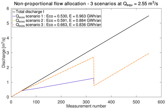
Figure 13.
Flow distribution for Scenarios 1–3 with = 2.55 m3/s. The values for the flow are implied by subtracting the total flow I from the ecosystem instream flow Q.
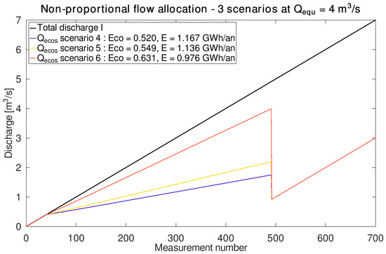
Figure 14.
Flow distribution for Scenarios 4–6 with = 4 m3/s. The values for the flow are implied by subtracting the total flow I from the ecosystem instream flow Q.
5. Discussion
5.1. Habitat Ecology for Brown Trout and Grayling
The accuracy of bathymetric surveys (longitudinal and transverse density of the measurements) influences the quality of the hydraulic model. Although the interpolation may smooth the bed bottom, our measurements appear accurate for integration into the hydraulic-habitat model. Clasing et al. (2023) [25] used a 30 m spacing for bathymetric surveys with RTK GPS, which is similar to the spacing chosen for this study. The macroroughness in the stream bed was integrated with a simple correction of the DTM, but obviously it does not represent precisely the dynamics. A more complex and precise approach integrates the bed objects by statistically correcting the WUA curves [26]. Substrate data are derived from spatial interpolation based on 33 georeferenced grading curves. It should be recognized that our method may potentially introduce a bias in the results due to the small amount of data and the simplicity of the interpolation. Even so, the aim of this model is to obtain an overall assessment score for habitats, expressed in WUA, so it can be assumed that a more detailed particle size distribution is not necessary. Overall, the simulation results seem consistent and fairly accurately reflect the hydraulic dynamics observed in the bathymetric and water velocity data for the study section. Nonetheless, there is room for improvement in the method by addressing the identified biases. Additionally, as noted by Padoan et al. (2024) [27], certain parameters, such as water temperature and fish feeding behaviors, are currently overlooked, reducing the reliability of our HSI calculation method. To enhance the predictive accuracy of the metapopulation model, addressing these gaps will be crucial and could significantly advance our understanding of habitat connectivity and population dynamics under human influence.
The results from the electrofishing survey indicate that hydropower operations in the studied sectors do not significantly affect trout of any life stage in the Birse River (Figure 4). This result is supported by the trout WUA curves (Figure 8 and Figure 9). Those curves show that the difference between the WUA values relative to the ecological flow required for the hydropower plant and the ones of the peak flows for the three life stages is negligible when compared with the total WUA available in the river (see Section 4.1 for quantitative details).
On the other hand, grayling seems to be largely affected by the hydropower operations of the Dynamo. The fact that in sector S2 we observed only 0+ individuals (Figure 5) indicates that the habitat of juvenile and adult grayling is affected by the operation of the Dynamo. The absence of juvenile and adult grayling in sector S2 is consistent with the trends observed in the WUA curves for grayling (Figure 10). These curves indicate that suitable habitat area starts to expand only when flows reach approximately 2–3 m3/s, reaching peak suitability at flows between 8 and 11 m3/s, well above the minimum residual flow requirement of 0.4 m3/s. The occurrence of 0+ grayling in sector S2, according to the WUA curves, is somewhat unexpected (Figure 5). The WUA for 0+ grayling peaks around 5 m3/s, thus lower than for older individuals, and exhibits gradual increments at flows around 0.5 m3/s. However, the discrepancy between the number of 0+ graylings found in sectors S1 and S2 confirms the lower suitability of sector S2.
These findings suggest that, in the absence of the hydroelectric structure, grayling would likely experience substantial benefits from increased habitat availability in the studied sections. Consequently, a partial restoration of the stream dynamics impacted by the hydroelectric structure, particularly through an augmentation in flow resulting from a non-proportional allocation of residual flows, is likely to yield a favorable outcome for the local grayling population. Although perhaps not to the same degree, it is noteworthy to emphasize that trout would also benefit from an increase in residual flows.
5.2. Ecohydrological and Economic Analysis of the Dynamo Power Plant
The hydroelectric production data embedded in the Matlab code exhibits a bias. Specifically, Scenarios 4–6, which utilize a 4 m3/s equipped flow, inappropriately use the same production curve as Scenarios 1–3 with the equipped flow of 2.55 m3/s, resulting in inaccuracies. Hourly flow data sourced from “La Charrue” station undergo extrapolation to catchment areas, introducing deviations. Moreover, the critical thresholds derived from WUA curves for juvenile and adult trout may be inaccurate due to manual calibration. Perona et al. (2021) [28] reported that relying solely on the fish habitat suitability indicator can introduce bias, as it depends only on the WUA critical threshold. Furthermore, our analysis, which focuses only on brown trout for the habitat sub-indicator, may bias results by neglecting other aquatic and terrestrial species, as suggested by Perona et al. (2021) [28]. Our findings demonstrate that graylings have distinct ecological preferences compared with brown trout, particularly visible in their WUA curves, which differ significantly. Therefore, future studies may need a reduction in the influence of the brown trout factor or the incorporation of additional species into the Eco factor to better approximate the balance of actual stream ecology. A more comprehensive approach could involve assigning different weights to different fish species to determine an average optimum of the Eco factor.
Regarding the flow allocation method at the Dynamo hydropower plant, transitioning from the “minimal flow release method” to an alternative approach inevitably leads to a reduction in hydroelectric production. This is because the current method maximizes water discharge, thereby achieving the highest possible energy output. According to Table 2 and the Swiss 2050 small-scale hydropower plant development strategy outlined in the introduction, even a 10% reduction in hydroelectric production, as seen in Scenario 1, may already be excessive. Consequently, Scenarios 2 and 3 may result in unsustainable production losses. However, maintaining a fixed ecological flow presents the worst-case scenario from an environmental perspective with an Eco-index of 0.385. The minimal flow release method is no longer relevant to Switzerland’s current objectives of restoring fish migration [6,29]. If the hydropower plant’s capacity remains unchanged, Scenario 1 (Figure 11) seems the most suitable option, as it is more reliable and has fewer economic impacts compared with Scenarios 2 and 3. However, if the capacity is increased to 4 m3/s, Scenario 5 would exceed the plant’s previous hydroelectric output at a constant ecological flow (1.136 GWh/year instead of 1.07 GWh/year) while also providing increased environmental benefits with an Eco-index of 0.549. Among Scenarios 4, 5, and 6, Scenario 5 (Figure 12) strikes a commendable balance between heightened environmental benefits and increased hydroelectric production. It is essential to carefully evaluate each hydroelectric scheme to reconcile ecological and economic imperatives. In some cases, the hydropower plant may already be operating at full capacity, making any increase in the equipped flow unfeasible.
The requirements of hydroelectric production limit the environmental benefit in accordance with the 2050 energy strategy [7]. Hence, it is worth exploring the option of covering canals with photovoltaic panels (PVs) to increase energy efficiency, as suggested by McKurin et al. (2021) [30]. Fully covering the Dynamo feeder channel with PVs could potentially yield a production of 0.143 GWh/year, assuming a 20% performance gain [31]. This additional production could become a convenient supplement of generated electricity for the Dynamo.
Figure 13 and Figure 14 demonstrate that optimal flow allocation involves a gradual increase in water inflow into the river until it reaches the equipped flow on the channel side. Subsequently, it decreases to the minimum ecological flow, presenting a significant disparity that could pose implementation challenges. One potential solution is to progressively adjust the flow regime at this juncture, either by reducing or increasing it, to mitigate the risk of fish stranding. In Scenarios 2 and 3 (Figure 13), curves are very similar. Despite this similarity, there exists a notable gap between the scenarios, as outlined in Table 2. The concern arises from the fact that inaccurate implementation could have a significant impact on both economic and ecological outcomes. Achieving this level of precision during implementation at the dam water intake may prove challenging. Therefore, before selecting a scenario for implementation in a hydroelectric scheme, it may be crucial to ensure that the scenario possesses a flow allocation curve that is distinctly unique.
The implementation of non-proportional flow in hydropower plants presents an opportunity to enhance efficiency over traditional fixed-percentage release methods. Bernard et al. (2017) [32] described in their work how to manage hydromechanical gates for non-proportional allocation with a dynamic gate–water relationship. Technologies like AMIL gates, when integrated with a weir system, enable dynamic water distribution based on real-time environmental conditions. This setup can optimize energy production while maintaining ecological integrity by allowing adaptive environmental flows without additional energy input. Recent studies, such as those by Martel et al. (2023) [33], propose an alternative to gate systems that involve asymmetric plate geometries mounted at water intakes. This system allows to regulate non-proportional flow distribution without additional operational costs. This hydrodynamic-based solution ensures minimal impact on energy consumption and offers flexibility for both storage and non-storage hydropower plants. Despite these pros, some challenges remain, such as refining the design of intake structures to achieve specific flow redistribution patterns or ensuring the long-term stability of these systems. To fill these gaps, there is a need for further research and testing of new reliable implementation.
6. Conclusions
The findings of this study highlight a non-linear relationship between electricity production and the quality of river habitat. By implementing a non-proportional flow allocation method instead of a fixed minimum residual flow one, it is possible to maintain high levels of electricity production while simultaneously enhancing the habitat quality of rivers. The presented results are significant and consistent with the ones obtained by previous research that suggested that Switzerland could make progress toward its 2050 energy objectives while including legally mandated ecological integrity of its waterways [10,11,28]. This study suggests that the combination of this approach with other measures (e.g., turbine upgrades, reduced energy loss, and introduction of photovoltaic panels covering the headrace channel) could bring Switzerland closer to reaching its energy targets. By focusing on a small hydropower plant and without considering storage mechanics, this approach can be further extended to storage system hydropower plants [34].
Additionally, it is important to recognize that this analysis, which emphasizes brown trout for the habitat sub-indicator, may have introduced a bias when underestimating the ecological needs of other aquatic species. While our study focuses on trout as a foundational element in the ecological and economic model to develop the methodology, future research should consider incorporating the other local species living in the reach (e.g., grayling for the presented case) into the Eco factor to reflect the overall stream ecology more accurately. This more comprehensive approach might involve the application of different weights to various fish species to determine an optimal balance.
We believe that our study serves as a valuable starting point to explore the application of non-proportional flow allocation across the different types of hydropower plants that impact waterways in Switzerland and beyond.
Author Contributions
Conceptualization, R.A., P.D.C. and F.F.; methodology, R.A., P.D.C., G.D.C. and F.F.; software, G.D.C. and F.F.; validation, P.D.C., F.F. and G.D.C.; formal analysis, R.A.; investigation, R.A.; resources, F.F.; data curation, R.A.; writing—original draft preparation, R.A.; writing—review and editing, R.A., F.F., G.D.C. and P.D.C.; visualization, R.A., F.F. and G.D.C.; supervision, P.D.C., F.F. and G.D.C.; project administration, R.A., F.F. and G.D.C.; funding acquisition, F.F. and G.D.C. All authors have read and agreed to the published version of the manuscript.
Funding
This research received no external funding.
Institutional Review Board Statement
Not applicable.
Informed Consent Statement
Not applicable.
Data Availability Statement
Data are contained within the article.
Acknowledgments
Gratitude to ENV’s Amaury Boillat, Alain Saner, and Florian Battilotti. Thanks to Paolo Perona for co-authoring references. Special thanks to Francesca Padoan for her meticulous review of the work. Appreciation to Joris Weber, Elias Valenti, Nicoletta Trabucchi, Mathilde Boross, Iacopo Aiolfi, and Jonathan Molina at EcoEng SA for their invaluable support. Thanks to Maryline der Stefanian’s data sharing and hydroelectric station visit. Their contributions were crucial. Many thanks to all.
Conflicts of Interest
The authors declare no conflicts of interest.
Abbreviations
The following abbreviations are used in this manuscript:
| FOEN | Federal Office of the ENvironment |
| HSI | Habitat Suitability Index |
| WUA | Weighted Usabel Area |
| IHA | Indicators of Hydrological Alteration |
| S1 | Sector S1 is situated downstream of the studied sector (see Figure 3). |
| S2 | Sector S2 is situated midstream of the studied sector (see Figure 3). |
| Mean flow of the flow duration curve at day 347. [m3/s] | |
| Current operating flow rate of the hydropower plant. [m3/s] | |
| Power output of the Dynamo hydropower plant. [J/s] | |
| Overall efficiency of the hydroelectric plant. [−] | |
| Density of water (considered constant). [kg/m3] | |
| Gravitational acceleration. [m/s2] | |
| Average net head of the Dynamo hydropower plant. [m] | |
| I | Upstream flow coming to the dam. [m3/s] |
| Upstream flow value at which competition between ecological and economic | |
| indices begins. [m3/s] | |
| Upstream flow value where competition between ecological and economic | |
| indices ends. [m3/s] | |
| Current ecosystem flows (river side). [m3/s] | |
| Minimum ecological flow (river side). [m3/s] | |
| Maximum operating flow (channel side). [m3/s] | |
| Minimum operating flow (channel side). [m3/s] | |
| Wetted area [m2] | |
| a | Adimensional parameter (Fermi function) affecting the shape of the curve. |
| b | Adimensional parameter (Fermi function) affecting the shape of the curve. |
| c | Adimensional parameter (Fermi function) fixing the curve arriving point at |
| . In this study, it is fixed at 1. | |
| i | Adimentional parameter (Fermi function), fraction of water left for the ecosystem |
| when (start of the competition between ecological and economic indices). | |
| j | Adimentional parameter (Fermi function), fraction of water left for the ecosystem |
| when (end of the competition between ecological and economic indices). | |
| Rate of non Attainment, part of the days for which the IHA deviate outside | |
| plus/minus one standard deviation, and the coefficient of variation. | |
| Coefficient of Variation, ratio between the standard deviation and the mean of the IHA. | |
| k | IHA indicator. |
| Root mean square distances between the simulated and natural . | |
| Root mean square distances between the simulated and natural . | |
| maximum number of consecutive days in which the river flow is below the critical | |
| WUA threshold for juvenile trouts. | |
| maximum number of consecutive days in which the river flow is below the critical | |
| WUA threshold for adult trouts. | |
| Eco | Dimensionless and synthetic ecohydrological indicator. |
| S | Non-proportional flow allocation scenario. |
| E | Hydroelectricity produced per year [GWh/year] |
| Current scenario using a fixed ecological flow method and an equipped | |
| flow of 2.55 m3/s. |
References
- Office Fédérale de L’énergie OFEN. Les Faits sur la Petite Hydraulique. OFEN. 2020. Available online: https://www.bfe.admin.ch/bfe/fr/home/versorgung/erneuerbare-energien/wasserkraft/kleinwasserkraft.exturl.html/aHR0cHM6Ly9wdWJkYi5iZmUuYWRtaW4uY2gvZnIvcHVibGljYX/Rpb24vZG93bmxvYWQvMTAzNTY=.html (accessed on 5 February 2024).
- Office Fédérale de L’énergie OFEN. Potentiel Hydroélectrique de la Suisse. OFEN. 2020. Available online: https://plattform-renaturierung.ch/wp-content/uploads/2019/09/Wasserkraftpotenzial_Schweiz_f.pdf (accessed on 5 February 2024).
- Di Giulio, M.; Angelone, S. Fiches sur l’aménagement et l’écologie des cours d’eau: Amélioration de la dynamique. OFEV. 2012. Available online: https://www.bafu.admin.ch/dam/bafu/fr/dokumente/wasser/uw-umwelt-wissen/merkblatt-sammlungwasserbauundoekologie.pdf.download.pdf/recueil_des_fichessurlamenagementetlecologiedescoursdeau.pdf (accessed on 10 December 2023).
- Lin, Q. Influence of Dams on River Ecosystem and Its Countermeasures. J. Water Resour. Prot. 2011, 2011, 3779. [Google Scholar] [CrossRef]
- Bammatter, L.; Baumgartner, M.; Greuter, L.; Haertel-Borer, S.; Huber, G.M.; Nitsche, M.; Thomas, G. Renaturation des eaux suisses: Plans d’assainissement des cantons dès 2015. OFEV. 2015. Available online: https://www.bafu.admin.ch/dam/bafu/fr/dokumente/wasser/fachinfo-daten/die_sanierungsplaenederkantoneab2015.pdf.download.pdf/plans_d_assainissementdescantonsdes2015.pdf (accessed on 2 April 2024).
- Estoppey, R.; Kiefer, B.; Greuter, L.; Kummer, M.; Lagger, S.; Aschwanden, H. Débit résiduel convenable, comment les déterminer? OFEV. 2000. Available online: https://www.bafu.admin.ch/dam/bafu/fr/dokumente/wasser/uv-umwelt-vollzug/angemessene_restwassermengenwiekoennensiebestimmtwerdenwegleitun.pdf.download.pdf/debits_residuelsconvenables-commentpeuvent-ilsetredeterminesinst.pdf (accessed on 15 December 2023).
- Pfammatter, R.; Wicki, N.S. Energieeinbussen aus Restwasser-Bestimmungen—Stand und Ausblick; Association Suisse pour l’Aménagement des Eaux: Zürich, Switzerland, 2018. [Google Scholar]
- Perona, P.; Dürrenmatt, D.J.; Tron, S.; Characklis, G.W. Obtaining natural-like flow releases in diverted river reaches from simple riparian benefit economic models. J. Environ. Manag. 2013, 118, 161–169. [Google Scholar] [CrossRef] [PubMed]
- Gorla, L.; Perona, P. On quantifying ecologically sustainable flow releases in a diverted river reach. J. Hydrol. 2013, 489, 98–107. [Google Scholar] [CrossRef]
- Razurel, P.; Gorla, L.; Tron, S.; Niayifar, A.; Crouzy, B.; Perona, P. Non-proportional Repartition Rules Optimize Environmental Flows and Energy Production. Water Resour. Manag. 2018, 30, 207–223. [Google Scholar] [CrossRef]
- Razurel, P.; Gorla, L.; Tron, S.; Niayifar, A.; Crouzy, B.; Perona, P. Improving the ecohydrological and economic efficiency of Small Hydropower Plants with water diversion. Adv. Water Resour. 2018, 113, 249–259. [Google Scholar] [CrossRef]
- Tschurr, F.; Mülchi, R.; Kotlarski, S.; Fischer, A.; Schlegel, T.; Duding, O.; Rajczak, J. Changements Climatiques Dans le Canton du Jura: Ce que l’on Sait et ce qui est Attendu Dans le Futur; NCCS National Center for Climate Services: Hague, The Netherlands, 2021. [Google Scholar]
- Hausmann, M. Petite Centrale hydroéLectrique de Courrendlin “Dynamo”, Analyse Sommaire; Internal report. Unpublished work; Office Fédérale de l’ENergie OFEN: Ittigen, Switzerland, 2012. [Google Scholar]
- Detert, M.; Weitbrecht, V. User Guide to Gravelometric Image Analysis by BASEGRAIN; Taylor and Francis Group: London, UK, 2013. [Google Scholar]
- Fehr, R. Einfache Bestimmung der Korngrössenverteilung von Geschiebematerial mit Hilfe der Linienzahlanalyse. Schweiz. Ing. Archit. 1987, 105, 1104–1109. [Google Scholar]
- Bovee, K.D. Development and Evaluation of Habitat Suitability Criteria for Use in the Instream Flow Incremental Methodology. In National Ecology Center, Division of Wildlife, Contaminant Research, Fish, and Wildlife Service; U.S. Department of the Interior: Washington, DC, USA, 1986. [Google Scholar]
- Plomb, J.; Zaugg, B. Rétablissement de la Migration du Poisson-Planification stratéGique; Federal Office for the Environment FOEN: Bern, Switzerland, 2021. [Google Scholar]
- Zaugg, B. Liste Rouge des Espèces Menacées en Suisse: Poisson et Cyclostomes; Federal Office for the Environment FOEN: Bern, Switzerland, 2022. [Google Scholar]
- Souchon, Y.; Trocherie, F.; Fragnoud, E.; Lacombe, C. Les modèles numériques des microhabitats des poissons: Application et nouveaux développements. Rev. Des Sci. L’Eau 1989, 2, 807–830. [Google Scholar]
- Mallet, J.P.; Lamouroux, N.; Sagnes, P.; Persat, H. Habitat preferences of European grayling in a medium size stream, the Ain river, France. JFB 2000, 2, 807–830. [Google Scholar] [CrossRef]
- Nestler, J.M.; Milhous, R.T.; Payne, T.R.; Smith, D.L. History and review of the habitat suitability criteria curve in applied aquatic ecology. River Res. Appl. 2019, 35, 1155–1180. [Google Scholar] [CrossRef]
- Richter, B.D.; Baumgartner, J.V.; Powell, J.; Braun, D.P. A Method for Assessing Hydrologic Alteration within Ecosystems. Conserv. Biol. 1996, 10, 11634174. [Google Scholar] [CrossRef]
- Bizzi, S.; Pianosi, F.; Soncini-Sessa, R. Valuing hydrological alteration in multi-objective water resources management. J. Hydrol. 2012, 472473, 277–286. [Google Scholar] [CrossRef]
- Capra, H.; Breil, P.; Souchon, Y. A New Tool to Interpret Magnitude and Duration of Fish Habitat Variations. Regul. Rivers Res. Manag. 1995, 10, 281–289. [Google Scholar] [CrossRef]
- Clasing, R.E.; Arumí, J.L.; Caamaño, D.; Alcayaga, H.; Medina, Y. Remote Sensing with UAVs for Modeling Floods: An Exploratory Approach Based on Three Chilean Rivers. Water 2023, 15, 1502. [Google Scholar] [CrossRef]
- Niayifar, A.; Oldroyd, H.; Lane, S.N.; Perona, P. Modeling Macroroughness Contribution to Fish Habitat Suitability Curves. Water Resour. Res. 2018, 54, 9306–9320. [Google Scholar] [CrossRef]
- Padoan, F.; Calvani, G.; De Cesare, G.; Brodersen, J.; Robinson, C.T.; Perona, P. Ecological and biogeomorphological modelling of brown trout (Salmo trutta L.). In River Research and Applications; Wiley Online Library: Hoboken, NJ, USA, 2024. [Google Scholar]
- Perona, P.; Niayifar, A.; Schwemmle, R.; Razurel, P.; Flury, R.; Winz, E.; Barry, D.A. Frontiers of (Pareto) Optimal and Sustainable Water Management for Hydropower and Ecology. Front. Environ. Sci. 2021, 9, 703433. [Google Scholar] [CrossRef]
- Office Fédéral de L’environnement OFEV. Rétablissement de la Migration du Poisson. OFEV. 2022. Available online: https://www.bafu.admin.ch/dam/bafu/fr/dokumente/wasser/uw-umwelt-wissen/wiederherstellung-fischwanderung.pdf.download.pdf/UW-2205-F_Fischwanderung.pdf (accessed on 21 March 2024).
- McKuin, B.; Zumkehr, A.; Ta, J.; Bales, R.; Viers, J.H.; Pathak, T. Energy and water co-benefits from covering canals with solar panels. Nat. Sustain. 2021, 4, 609–617. [Google Scholar] [CrossRef]
- Solar Thermal Shows Highest Energy Yield Per Square Metre. Available online: https://solarthermalworld.org/news/solar-thermal-shows-highest-energy-yield-square-metre/ (accessed on 30 August 2023).
- Bernhard, F.; Perona, P. Dynamical Behavior and Stability Analysis of Hydromechanical Gates. J. Irrig. Drain. Eng. 2017, 143, 04017039. [Google Scholar] [CrossRef]
- Martel, S.; Saharei, P.; De Cesare, G.; Perona, P. Dynamic environmental flows using hydrodynamic-based solutions for sustainable hydropower. In Role of Dams and Reservoirs in a Successful Energy Transition; CRC Press: Boca Raton, FL, USA, 2023. [Google Scholar]
- Niayifar, A. Dynamic water allocation policies improve the global efficiency of storage systems. Adv. in Water Resour. 2017, 104, 55–64. [Google Scholar] [CrossRef]


Disclaimer/Publisher’s Note: The statements, opinions and data contained in all publications are solely those of the individual author(s) and contributor(s) and not of MDPI and/or the editor(s). MDPI and/or the editor(s) disclaim responsibility for any injury to people or property resulting from any ideas, methods, instructions or products referred to in the content. |
© 2024 by the authors. Licensee MDPI, Basel, Switzerland. This article is an open access article distributed under the terms and conditions of the Creative Commons Attribution (CC BY) license (https://creativecommons.org/licenses/by/4.0/).