1. Introduction
Continuously impacted by the effects of the climate crisis, urban dynamics and quality of life in cities are threatened by the growth and dependence on motorised vehicles. The need to enhance the efficiency of daily journeys and provide personal and communal benefits to city dwellers, combined with attributes that are opposite to motorised private transport, allows cycling to directly contribute to the 2030 Agenda for Sustainable Development and places this mode in the spotlight of transport planning as part of a solution for many urban problems [
1,
2].
The increasing emission of greenhouse gases (GHGs) presents a significant challenge, especially in the transport sector, which accounts for a substantial portion of total emissions in Europe and Portugal [
3]. The overreliance on private automobiles, widely acknowledged as a primary contributing factor, has resulted in severe environmental impacts, including air and noise pollution [
4]. In addition to carbon dioxide (CO
2) emissions, the combustion of fossil fuels also releases harmful pollutants such as particulate matter (PM) and nitrogen oxides (NOx). These have a severe impact on public health and lead to millions of premature deaths each year, particularly in urban areas across Europe [
5,
6].
The current focus on reducing greenhouse gas (GHG) emissions primarily revolves around replacing fossil fuels with cleaner alternatives, such as electric vehicles [
7,
8]. Studies indicate that transitioning to electric vehicles is crucial for meeting emission reduction targets set by the European Union and the Paris Agreement [
9]. However, a significant shift towards active transport modes is also necessary [
4,
10]. Specifically, promoting cycling can help decrease the reliance on cars for short-distance trips within cities, leading to a substantial shift in urban transportation patterns [
11,
12]. This shift could reduce local and global emissions [
13,
14].
From an individual perspective, the health-enhancing and economic benefits of cycling are well-known and widely accepted [
15,
16]. From the city’s perspective, which continues to grapple with limited space, congestion, and air pollution, cycling infrastructure requires significantly less space. It is often more cost-effective than building and maintaining car infrastructure [
17]. Hence, bicycles have become a crucial factor in reducing carbon emissions in transportation, especially for short urban trips of up to 15 min, which can be completed using cycling instead of private vehicles [
4]. The integration of cycling infrastructure with public transport networks further reinforces this role, as cyclists can conveniently access transportation hubs and continue their journey using higher-capacity modes, making bicycles an important feeder mode [
18,
19,
20]. This approach helps to reduce greenhouse gas emissions, improve air quality, and enhance urban living conditions, aligning with the European Union’s climate and environmental goals for 2030 and 2040 [
8,
9].
A cycling network infrastructure is crucial to promoting daily bicycle usage levels [
13,
21]. Considering the significant challenges posed by planning and implementing bicycle infrastructure in urban settings [
22], offering a practical method with well-detailed measures to assess the bikeability network can be an essential tool and guidance for urban planning professionals and municipalities involved in constructing, expanding, or enhancing cycling and related infrastructure. These methods are valuable for urban planning focused on decarbonisation, providing strategic support in the transition towards more sustainable transport systems. Therefore, encouraging bicycle use, transport electrification, and improved infrastructure for active modes could significantly contribute to achieving the sustainability goals [
4].
The main objective of this paper is to present a practical approach, followed by “how-to-do” measures, to assess bikeability based on GIS methodologies. Moreover, we carried out a case study using this experimental index for Póvoa de Varzim in Portugal. The main contribution of this approach is to integrate factors relatively underused in bikeability indexes, such as bicycle parking features (density, typology, and amenities) and environmental features (noise and pollen). Because the parameters are meticulously detailed, this approach can be easily applied and adjusted for different contexts.
2. Background
Bikeability is a relatively recent concept developed from the established and consolidated concept of walkability [
15] and is relevant to sustainable mobility, specifically in promoting better sustainable urban transport planning. The variety of definitions of “bikeability” may cause some misunderstanding, mainly because it is used in distinct research fields such as public health, urban planning, and transportation [
23]. Considering the last one, bikeability encompasses several definitions, such as level of service [
24], level of traffic stress [
25], friendliness [
26], and accessibility [
27,
28]. Despite different definitions, there is an exact one that defines bikeability as “an assessment of an entire bikeway network’s perceived comfort, convenience, and accessibility to key destinations” [
24]. The authors argue that this goes beyond the assessment of comfort and safety of a segment; however, such characteristics are also encompassed. Regarding methods, “bikeability” is typically applied as an indexation of examined environmental features in a context where cycling is prioritised [
29]. In essence, it gauges the overall suitability and support provided by the examined environment for someone opting for cycling as their preferred means of transportation.
Assessment processes involving multiple factors, such as bikeability indexes, have a critical stage: determining the importance of each factor. Additionally, the significance of each factor may vary for different decision-makers or contextual settings. Therefore, defining the relative importance in the decision-making process is essential, typically achieved by assigning specific weights to each factor. Standard procedures in bikeability indexes include ranking the factors according to their order of importance [
26,
30,
31] and employing the point-scale-based method [
32,
33].
Once the measurements for each indicator are obtained, the next step is to normalise them for equitable treatment. The literature identifies two primary methods for this normalisation. One method involves additive weighting, equal weights, or weighting schemes [
30,
33], while the other employs a hierarchical structure using pairwise comparisons or regression models [
34,
35]. Both approaches face limitations due to individual perception [
34]. However, pairwise comparisons can more accurately capture and quantify decision-makers’ subjective preferences, making them more suitable for scenarios with multiple criteria and alternatives [
36], such as assessing the bikeability of a network.
A bicycle network can be expressed as an interconnected system of streets where cycling is not forbidden and different levels of comfort and convenience are provided. Hence, a bicycle network consists of paths designed for cyclists, including exclusive paths and shared ones where cyclists and other road users use the same space [
37]. Based on guidelines about homogeneity of masses and velocities [
38], we argue that two distinct expressions should treat these perspectives with dichotomic meaning. On the one hand, spaces shared with fellow users of cycle facilities (e.g., cargo bikes, light mopeds, mobility scooters, horse riders) should be referred to as shared spaces. On the other hand, when space division involves a motorised vehicle (heavy or light), the term coexistence should be applied.
Assessment methods for bicycle networks can be location-based or facility-based, relying on qualitative evaluations or quantitative analysis to understand cyclists’ perceptions and evaluate the conditions for cycling [
23]. Based on our previous work, it is possible to affirm that the standard factors in bikeability assessment are Cycling Infrastructures, Safety, and Accessibility. Cycling infrastructures encompass aspects related to the availability, quantity, quality, and typology of infrastructures and facilities [
25,
26,
27,
31,
39,
40], geometric design [
24,
35,
40], and bicycle parking [
35]. The accessibility factor involves aspects related to land use [
24,
27,
30,
31,
35]. The safety factor encompasses elements of the relationship between the physical and functional characteristics of cycling infrastructures [
26,
30,
35], as well as characteristics of traffic flow [
24,
35,
40] and conflict points with other modes of transportation [
31,
35]. Other relevant aspects of cycling, such as topography [
26,
30,
31,
35,
40] and landscape aesthetics [
26,
35,
39,
40], are not typically grouped into a specific factor, often subsumed under the abovementioned factors. Additionally, air quality and noise factors are rarely considered in bikeability indices [
23].
This paper broadens its focus from the conventional three factors—Cycling Infrastructures, Safety, and Accessibility—to encompass six critical factors: Accessibility, Infrastructure, Parking Infrastructure, Road Features, Surrounding Environment, and Traffic. Accessibility has been expanded beyond land use, incorporating variables related to multimodality. Infrastructure has been organised with variables that reflect the physical design features of cycling infrastructure (on-road features). In addition, a specific factor was created for aspects related to bicycle parking (spatial distribution, typology, and facilities). Road features encompass characteristics of roads in a less direct way than dedicated infrastructure. The surrounding environment covers air quality, noise, and landscape aesthetics. Safety brings together aspects related to the traffic flow.
The expansion from three to six factors in this study reflects a more comprehensive approach to understanding the multifaceted nature of bikeability. Accessibility, now broadened to include variables related to multimodality, is crucial for promoting cycling by facilitating seamless integration with other forms of transport, such as walking and public transport [
17,
41]. This expanded view recognises that a well-connected, accessible urban network is fundamental for increasing bicycle use.
The infrastructure factor explicitly addresses the physical features of cycling paths and lanes and is pivotal in making cycling safer and more convenient. Well-designed cycling infrastructure, including segregated bike lanes and clear signage, has significantly increased cycling uptake by reducing conflicts with motor vehicles and enhancing the overall cycling experience [
17,
30]. Additionally, the availability and quality of parking facilities, such as spatial distribution, typology, and security, are essential for improving the convenience of cycling [
42].
The inclusion of road features acknowledges that overall road conditions, such as lane width, surface quality, and intersection design, also impact cyclists’ comfort and safety. While not specifically designed for cycling, roads are considered either bike-friendly or risky based on the quality of these factors, which influences cyclists’ experiences and choices [
41,
43].
Similarly, the surrounding environment, which considers elements such as air quality, noise levels, and landscape aesthetics, profoundly impacts the attractiveness of cycling routes. Cyclists prefer visually appealing, quieter routes with cleaner air, as these factors contribute to their physical well-being and overall cycling experience [
41].
Safety is crucial when considering the feasibility of cycling, especially in urban areas. Factors such as the amount of motor vehicle traffic and speed limits are indicators of safety, with higher volumes and speeds leading to a lower sense of safety for cyclists [
17,
44].
3. Case Study in Póvoa de Varzim, Portugal
3.1. The Target Area for Testing Bikeability Assessment
The municipality of Póvoa de Varzim, with a population of 64,320 inhabitants, covers a territory of 82.81 km2 located in the Porto Metropolitan Area in the northern region of Portugal. The case study focuses on the central region of the city, which is bordered to the north by an urban hiatus, to the east by an express motorway (A28), to the south by the city of Vila do Conde, with which it forms a conurbation, and to the west by the Atlantic Ocean.
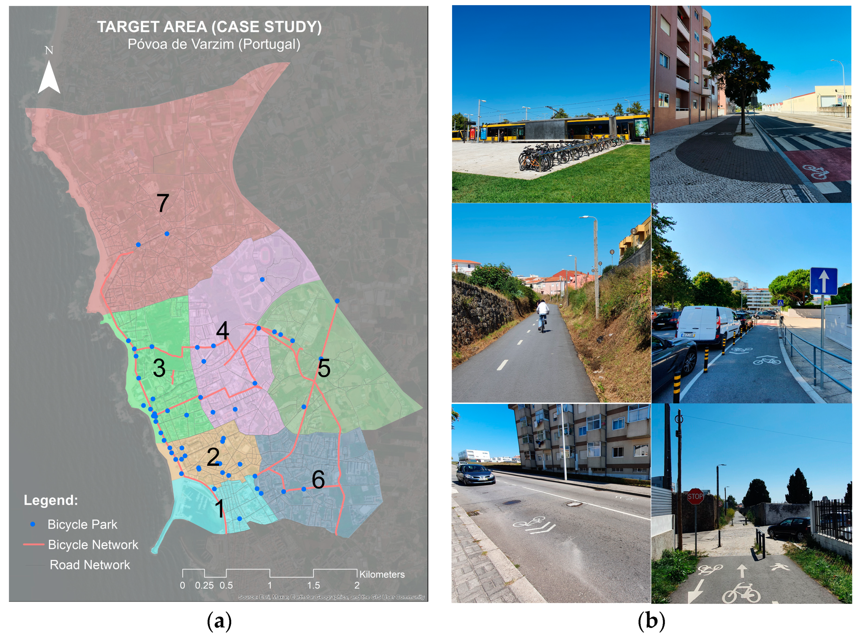
The city’s growth followed a pattern from inland to the coast (
Figure 1a), with the original nucleus (1) located in the southern part of the study area. The old town’s narrow and winding alleys, dating back to the 14th century, can still be found in this region. The central region (2) is characterised by the service sector and streets lined with traditional commerce. A highly urbanised region lies to the north (3) of the central region, characterised by streets that run parallel to the coastline. This is a beach area with tall buildings concentrated in its northern portion. To the east of this area lies a more recently planned region (4), where the city park is located. West of the original nucleus are two interior zones with distinct characteristics, one with a rural aspect (5) and another further south with diverse occupancy typologies (6). A coastal urban zone of residential character exhibiting an organic growth pattern lies at the northernmost tip (7).
The city of Póvoa emerges as a promising case study for several reasons. Firstly, due to the dedicated cycling infrastructure, the municipality features a network of cycle lanes extending over 30 km [
45]. Secondly, the city administration is committed to initiatives aimed at reversing the trends of car-centric urban planning, specifically by providing adequate infrastructure for regular bicycle use (
Figure 1b). Additionally, the geography and seasonality of the city make cycling an attractive alternative for urban travel, considering the moderate distances, favourable topography, and coastal characteristics that can enhance bicycle usage during certain times of the year.
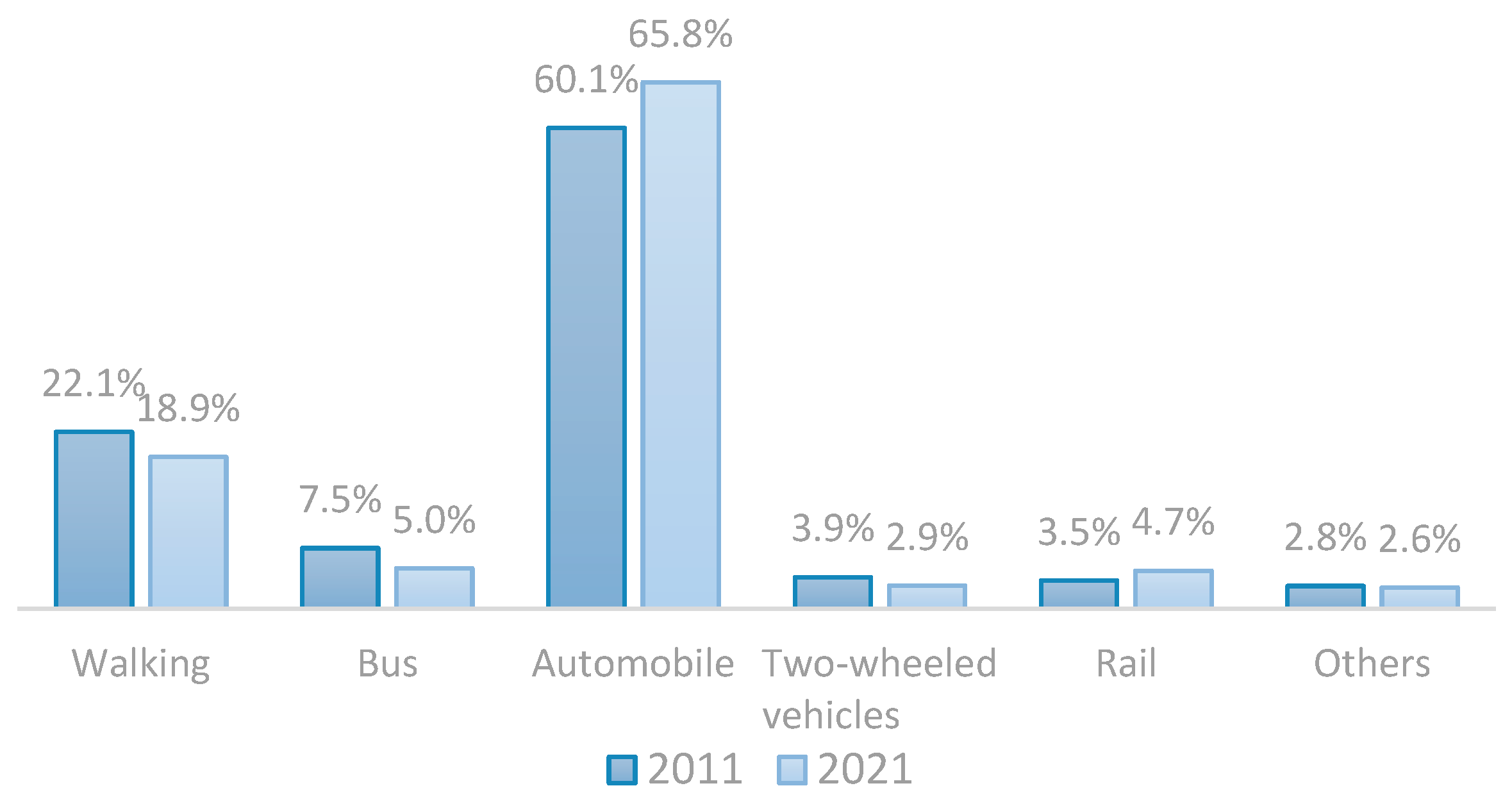
The analysis of the modal split through data from the 2011 and 2021 censuses in
Figure 2 reveals an increase of over 5% in car usage, while active modes of transportation, such as walking and two-wheeled vehicles (primarily bicycles), have decreased [
46]. Although these data do not exclusively pertain to urban travel, they suggest that travel patterns in the area still heavily rely on cars. The residual share dedicated to cycling indicates an inconsistency between existing infrastructure and cyclists’ needs. Still, it is also influenced by cultural factors such as resistance or hesitancy to adopt cycling as a means of transportation, a trend that has been observed in other cities in Portugal [
47].
The approach outlined in this study has the potential to aid urban planners in Póvoa do Varzim and other comparable starter cities by helping with gauging the network’s bikeability through segment evaluations. This insight facilitates the creation of comprehensive infrastructure enhancement strategies, including pinpointing new connections and amenities to encourage cycling and avoiding fragmented and disconnected infrastructure segments.
3.2. Methodological Approach
The study uses a method that combines aspects of both spectrum family methods. It considers variables from the facility-based methods (some from accessibility and infrastructure factors) and location-based ones (from infrastructure, road features, and surrounding environment factors). Additionally, the method uses both quantitative and qualitative measures to evaluate the cycling network at the segment level, resulting in a comprehensive network segment-based assessment. While this method shares more characteristics with facility-based methods, its features categorise it more accurately as a hybrid method. A four-step approach was used to collect and process data for each variable, illustrated in
Figure 3 below and described in the following paragraphs. It is noteworthy to highlight the use of clustering into two macro stages to aid the interpretation of the tables detailing each variable in the sections that address each factor.
After establishing the criteria and variables to be considered, we collected initial data by reviewing documents published by the municipality and technical reports. This involved gathering information on bicycle racks, cycle routes, bus stops, noise maps, and traffic volume. The collected data were then organised using a Geographic Information System (GIS), with the urban road network obtained from shapefiles from the Open Street Map (OSM) platform as a reference. We meticulously compared these data with the actual street layout and made necessary corrections to represent the existing urban fabric accurately. Following the exhaustion of official data sources, we proceeded with online data collection using Street View Imagery (SVI) to gather information on variables that were easier to detect or less likely to change, such as bus stop layout, number of traffic lanes, parking lot layout, green parks, and water bodies. The SVI-based survey provided valuable guidance for the subsequent steps in the process.
In the second step, we verified all the characteristics related to the variables for each network segment through several field campaigns. Some variables had data collected exclusively during these campaigns due to the absence of official data or a lack of visibility in the SVI (e.g., buffer space, cycle lane width, surface smoothness, tree pollen). Most variables were supplemented with data obtained and verified through multiple collection methods. This is evident in
Table 1 below, confirming that the SVI is highly valuable for guiding field campaigns despite not providing full visibility.
In the third phase, we allocated the variables based on specific criteria for each one under consideration. To accomplish this, we utilised various methods to standardise the variables that comprise each factor, taking into account the perceptibility of the categories, which may be referred to as discrete or continuous. For variables with clearly defined categories, we either ranked them by importance or used a dichotomous classification. In cases where the categories or the impact of variation were not easily discernible, we employed a fuzzification process.
This process involved converting a set of values expressed on one scale into a comparable set expressed on a normalised scale. The result indicated the degree of membership in a set, ranging from 0 to 1, signifying a continuous increase from non-membership to full membership based on the criterion subjected to the fuzzification process. This process entailed applying functions that governed the variation between the initial inflexion point, from which the criterion’s scores began contributing to the decision, and the final inflexion point, beyond which further scores did not provide any additional contribution.
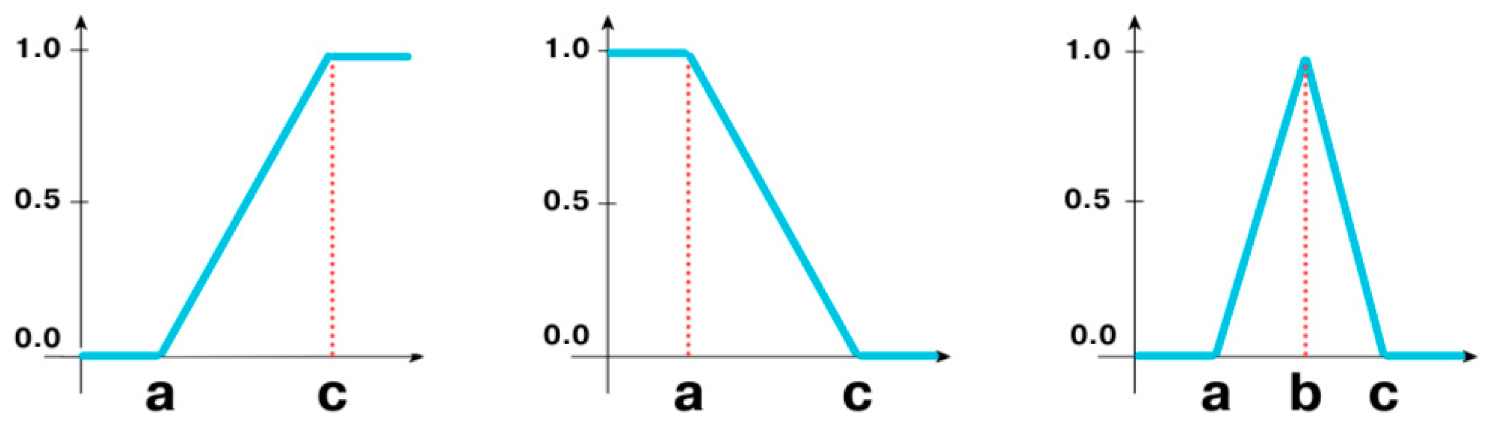
Figure 4 depicts the shapes of the membership functions, and the formulations for each are presented in expressions 1, 2, and 3, with the control points (a, b, c) visible. The selection of control points was a critical aspect of the fuzzification process, as it effectively calibrated the function for criteria and realities [
48].
The selection of appropriate membership functions depends on the nature of the factor being considered. In this study, we employed increasing, decreasing, and composite functions. The following paragraphs present examples to illustrate the reasoning behind each type of function, considering variables corresponding to each type of membership function.
Regarding the variable “cycle lane width,” it is essential to establish a threshold to differentiate between narrow and wide cycle lanes. For example, in the case of two-way cycle lanes, if the width of the segment is less than 2.5 m (x < a), the function’s value will be 0, indicating that the segment is unsuitable for bidirectional cycle traffic. If the width falls between 2.5 and 4.5 m (a ≤ x ≤ c), the membership function’s value will gradually increase from 0 to 1, indicating an increasing suitability of the segment for bidirectional bicycle traffic. If the width of the segment exceeds 4.5 m (x > c), the function’s value will be 1, signifying that the segment is fully suitable for a bidirectional cycle lane.
When assessing the “entries/exits” variable, it is essential to establish a threshold that distinguishes segments with high-access density from those with low-access density. If the density of entries and exits is less than 15 accesses per 100 m (x < a), the function’s value will be 1, indicating that the segment is highly suitable for bicycle traffic due to minimal interference from access points. If the density ranges between 15 and 30 accesses per 100 m (a ≤ x ≤ c), the membership function’s value will gradually decrease from 1 to 0, reflecting a decrease in the segment’s suitability as access density increases. Furthermore, if the density of entries and exits exceeds 30 accesses per 100 m (x > c), the function’s value will be 0, indicating that the segment is unsuitable for bicycle traffic due to excessive interference from access points.
A threshold was established to determine “canopy coverage,” distinguishing areas with low tree coverage and those with significant coverage. If the tree density is less than 8 trees per 100 m (x < a), the value of the function will be 0, indicating that the area is unsuitable as it provides little to no shade. If the density is between 8 and 14 trees per 100 m (a ≤ x ≤ b), the value of the function will gradually increase from 0 to 1 as the tree coverage increases, making the area more suitable for bicycle traffic. If the density is between 14 and 20 trees per 100 m (b ≤ x ≤ c), the function’s value will gradually decrease from 1 to 0, indicating a decline in the area’s suitability due to excessive tree density, which could pose risks to cyclists. When the tree density exceeds 20 per 100 m (x > c), the function’s value will be 0, signifying that the area is unsuitable due to risks associated with high tree density, such as slippery surfaces or increased maintenance.
In the fourth and final phase, the normalised values of each variable for each section of the urban network are organised into an attribute table, enabling them to be graphically represented in a GIS environment and facilitating the production of maps.
3.2.1. Accessibility
When considering cycling as a regular mode of transportation, high variability in activities within a region is a favourable built-environment feature, as mixed land use enhances the probability of multiple trips [
26,
30,
35].
Moreover, the synergy between bicycles and public transit depends on the level of integration between these modes. Bus stops and other passenger terminals are naturally predisposed to implementing bicycle parking. Such infrastructure increases a stop’s catchment area and extends the reach for the trip’s first and last legs [
18,
49]. The level of integration depends on the connections between a cycling axis and public transportation.
Furthermore, the number of bicycle parking spaces offered at train stations, bus terminals, or near bus stops influences the adoption of multimodal trips within the urban transportation system. The appropriated capacity of bicycle parking at public transportation terminals enhances the catchment area of these infrastructures and strengthens bicycles as a feeder mode. The availability of bicycle spaces at terminals becomes even more crucial for multimodal journeys when cyclists cannot bring their bicycles on the public transportation leg of their trip [
50,
51].
The variables considered in the accessibility factor are the connection to public transit, destination diversity, and parking spaces accessible from a transport hub. The data collection process for the variables is detailed in
Table 2.
3.2.2. Infrastructure
Linear infrastructure plays a crucial role in segregating cyclists from motorised traffic through dedicated lanes and bike paths. These infrastructures increase the likelihood of a person choosing cycling as a mode of transportation and a cyclist selecting a particular route [
38]. However, the absence of bike lanes and paths does not exclude the vocation of an urban road accommodating bicycle traffic. Every street is a cycling network segment; therefore, other factors (e.g., speed and traffic volume) can be observed and measured [
23].
Bicycle traffic can be disturbed by motorised and pedestrian traffic depending on the type of cycling infrastructure and its corresponding level of segregation. Using buffered spaces between cycling infrastructure and its surroundings can mitigate potential conflicts (e.g., cycling along a busy sidewalk, a bike lane along a traffic or parking lane, or a bike lane in a section with many pedestrian or vehicular accesses) [
23]. As a practical example, separating strips are extremely useful in preventing “dooring” incidents involving cyclists and sudden openings of vehicle doors.
Cycle lane width directly influences the capacity of the infrastructure and the safety and comfort conditions for users; the latter plays a role in cities where bicycle usage is not predominant [
23,
39]. Furthermore, physical barriers to protect cyclists and mitigate the risk of conflicts play a role in the exposure level associated with the intersection design (number of conflict points). We focused on design solutions that promote the perception of continuity in cycling infrastructure and unequivocally highlight bicycle flow preferences at the intersection (e.g., physical barriers, designated turning spaces such as a turn box or accumulation spaces, and bike box/queue box) [
23,
39].
Cycling infrastructures should be as flat as possible. A cycling route’s comfort and attractiveness are best when its segments’ slopes are minimised [
23,
39]. On the one hand, steep slopes directly influence the effort required by cyclists to complete a given route from a lower to a higher elevation. On the other hand, they also affect safety since they allow bicycles to develop high speeds when moving downwards [
40]. The slopes will vary according to the topography of the terrain in which the cycling network is located. In this regard, slopes and their extent should also be considered. Surface smoothness is a critical factor influencing riding comfort and safety. The type of material used in the tire–pavement interface and the condition of the surface, i.e., the presence of irregularities, can generate vibrations that affect riding comfort [
23,
39,
40]. Additionally, elements causing differences in depth exceeding two centimetres on the pavement are potential factors influencing surface regularity and, at times, may necessitate abrupt manoeuvres [
23].
Ensuring the availability of bicycle parking in a network segment is essential for any journey, especially for fostering cycling as a mode of transportation. It should be emphasised that the distribution of parking should align with relevant destinations for cyclists and in areas characterised by mixed land use [
17,
27,
35,
36]. In addition to availability, it is also essential to consider the quality of parking facilities provided for cyclists. This can be assessed through the type of existing infrastructure. The need for fully protected parking may be related to factors such as weather conditions, long-term parking, level of public safety, and type of bicycle; cyclists who use more expensive bicycles, especially electric-assisted ones, are more affected by the level of protection of parking [
17,
41]. Additionally, toilet and changing room facilities adjacent to bicycle parking areas significantly enhance the cycling experience, particularly for commuters [
41]. Access to these amenities supports cyclists’ comfort and convenience, enabling them to freshen up before or after their rides. The changing facility may be a separate structure near the parking area (e.g., public showers/toilets close to racks) or structures attached to more extensive parking facilities at transportation terminals.
The variables considered in the infrastructure factor include linear infrastructure, buffer space, protected intersections, slope, surface smoothness, bicycle parking density, bicycle parking typology, and toilet/changing room availability. The data collection process for these variables is detailed in
Table 3.
3.2.3. Road Features
The design and layout of urban infrastructure play a crucial role in facilitating safe and efficient cycling within cities. The bus stop position related to segregated cycling infrastructure can lead to conflicts between buses and the flow of bicycles. This situation becomes more problematic when considering infrastructures that allow bicycles to flow in opposite directions because they must be especially cautious about passengers waiting for public traffic who may not be aware of the two-way stream and bus manoeuvres. Ideally, bike lanes and paths should be implemented in the rear portion of bus stops to eliminate conflicts between the cyclist flow and buses [
52,
53].
The entry and exit of pedestrians and vehicles along cycling routes pose potential risks to cyclists, particularly in high densities areas where people may be focused on a specific activity (e.g., opening gates, focusing on motorised traffic, focusing on children, looking for keys) and may not notice the passage of bicycles. Cyclists must remain vigilant and adapt their speed to navigate these areas safely. This necessary behaviour can affect the flow of bicycles in the segment [
23,
38,
53].
The number of lanes is closely related to the road function, as it directly affects its capacity to accommodate motorised traffic volume and influences cycling conditions by impacting cyclists’ perceptions of safety [
24,
25,
40]. Although traffic volume varies over time, it was considered that the more lanes there are, the less conducive the road will be to cycling traffic.
Parking lot layout influences space availability and can affect cyclist safety by introducing potential conflicts with cars during entry and exit manoeuvres. Infrastructure designs that prioritise visibility and minimise interference between cycling and parking areas contribute to safer cycling environments [
35,
52,
53].
Furthermore, street lighting is a feature that influences both road safety and public security. Regarding the first one, the emphasis is on the need to see and be seen. This means road users must be able to identify paths and barriers for safe movement. Lighting also affects the sense of security; a well-lit environment can act as a deterrent against theft, burglary, and property damage [
38]. While easily measurable characteristics such as luminaire height and light source type are important considerations, the emphasis is on utilising measures that are easily recorded and already applied in existing indexes [
35].
The parking infrastructure factors consider the bus stop layout, entries/exits, number of traffic lanes, parking lot layout, and streetlights. The data collection process for these variables is detailed in
Table 4.
3.2.4. Surrounding Environment
The environment surrounding cycling pathways plays a significant role in shaping the overall cycling experience. Canopy coverage refers to the shade provided by trees aligned along a path. The number of trees must be sufficient to provide shade in intense sunlight. However, if the number of trees is too large, unfavourable situations may arise, such as the accumulation of leaves on the cyclists’ paths and drainage devices. It may lead to cyclists’ slips and falls and affect the frequency of maintenance on the segment [
38,
54].
Green parks or similar elements adjacent to cycling pathways enhance their attractiveness and enjoyment for cyclists. Gardens, squares, woodlands, and parks contribute to a scenic and idyllic environment, making cycling journeys more pleasant and rewarding [
26,
38,
39].
Despite being underestimated, noise pollution can be extremely harmful to health. In urban environments, vehicular traffic stands out as the primary source of noise to which cyclists are exposed. These noises can interfere with the cyclist’s perception of risks present on the road. Prolonged exposure over time increases stress levels and can impact cognitive and psychomotor abilities, which are crucial for the safe operation of a vulnerable two-wheeled vehicle [
41].
The presence of trees along a route and in green areas contributes to the attractiveness and comfort of a cycling path. For urban cyclists, trees can mitigate heat by reducing sun exposure. The idyllic environment also positively impacts recreational cyclists [
38,
39]. However, at some times of the year, especially in spring, and more markedly in some regions, trees can increase pollen concentration in the surroundings. These particles can irritate, particularly in the eyes and respiratory passages, posing a hindrance for individuals with allergies [
55]. In high concentrations, they may even affect those with no hypersensitivity to particles, thus serving as a deterrent for bicycle use. To assess the level of allergenicity, we considered a list of botanical species existing in Europe and predominant in the Portuguese territory, as shown in
Table 5.
Furthermore, water bodies adjacent to cycling pathways contribute to their attractiveness and environmental quality. These elements offer cooling effects during hot periods and humidify the surroundings in arid zones, enhancing the overall cycling experience. Additionally, water bodies add aesthetic value to routes, further enriching cyclists’ journeys [
38,
39].
The variables considered in the surrounding environment are canopy cover, green parks, noise, tree pollen, and water bodies.
Table 6 details the data collection and processing for these variables.
3.2.5. Safety
Managing motorised traffic speed and volume is essential for promoting cyclist safety and enhancing the cycling experience within urban environments. High speeds increase the frequency and severity of road accidents. This factor affects cycling mode because bicycles have unstable dynamics and lack crumple zones for impact absorption, so the cyclist is one of the most vulnerable road users [
24,
35]. The speed of a section was defined by the speed limit indicated on the road’s signs.
The daily traffic volume is another crucial aspect of traffic influencing cyclist safety. While low traffic volumes allow coexistence, the opposite makes separating bicycles from motorised vehicles necessary [
38,
53]. Ideally, the traffic stream should consist only of cars (light vehicles); thus, traffic counts incorporate conversion factors, and volumes are given in equivalent units. In traffic data collection, whether through traffic surveys or secondary sources (i.e., available counts), attention should always be given to the methodology employed in the surveys.
The variables considered in the traffic factor are motorised traffic speed and traffic volume. The data collection process for these variables is detailed in
Table 7.
3.3. Inspected Criteria and Resulting Map Views
In this section, we will present the results in the order of the factors considered in the index, which range from accessibility to the surrounding environment. Each aspect will be linked to the different zones of the target area, offering a comprehensive overview of the identified conditions. The 120.2 km of the urban network covered by this study is distributed as follows: Zone 1 (6.4%); Zone 2 (10.3%); Zone 3 (11.2%); Zone 4 (18.5%); Zone 5 (13.3%); Zone 6 (16.1%); and Zone 7 (24.2%). The score for each criterion assessed and the bikeability index range from 0 to 1. To provide a more concise overview of the results for the target area, we have divided the scores into five classes, as follows: “Very Low” (0.00–0.20); “Low” (0.21–0.40); “Moderate” (0.41–0.60); “High” (0.61–0.80); and “Very High” (0.81–1.00).
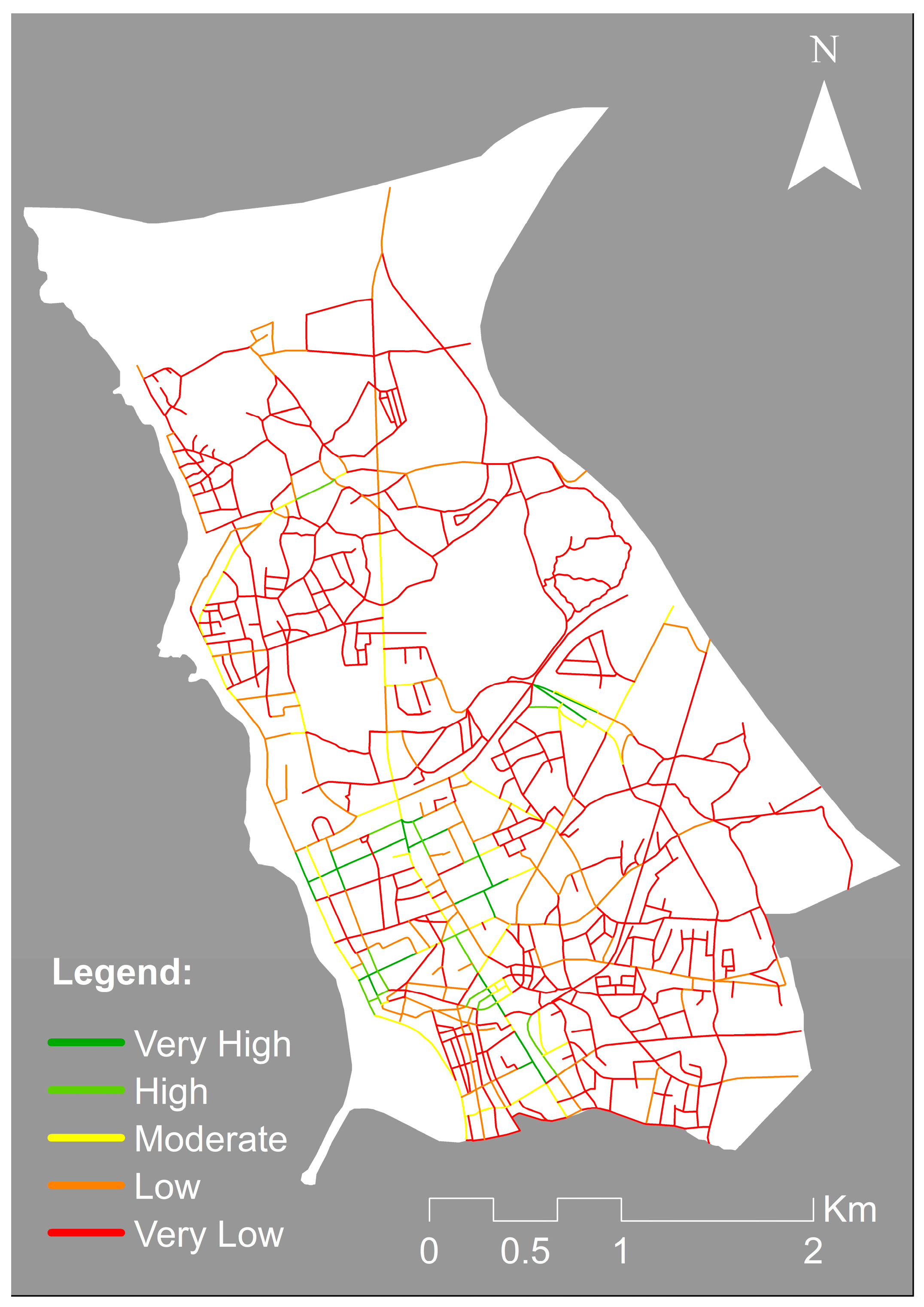
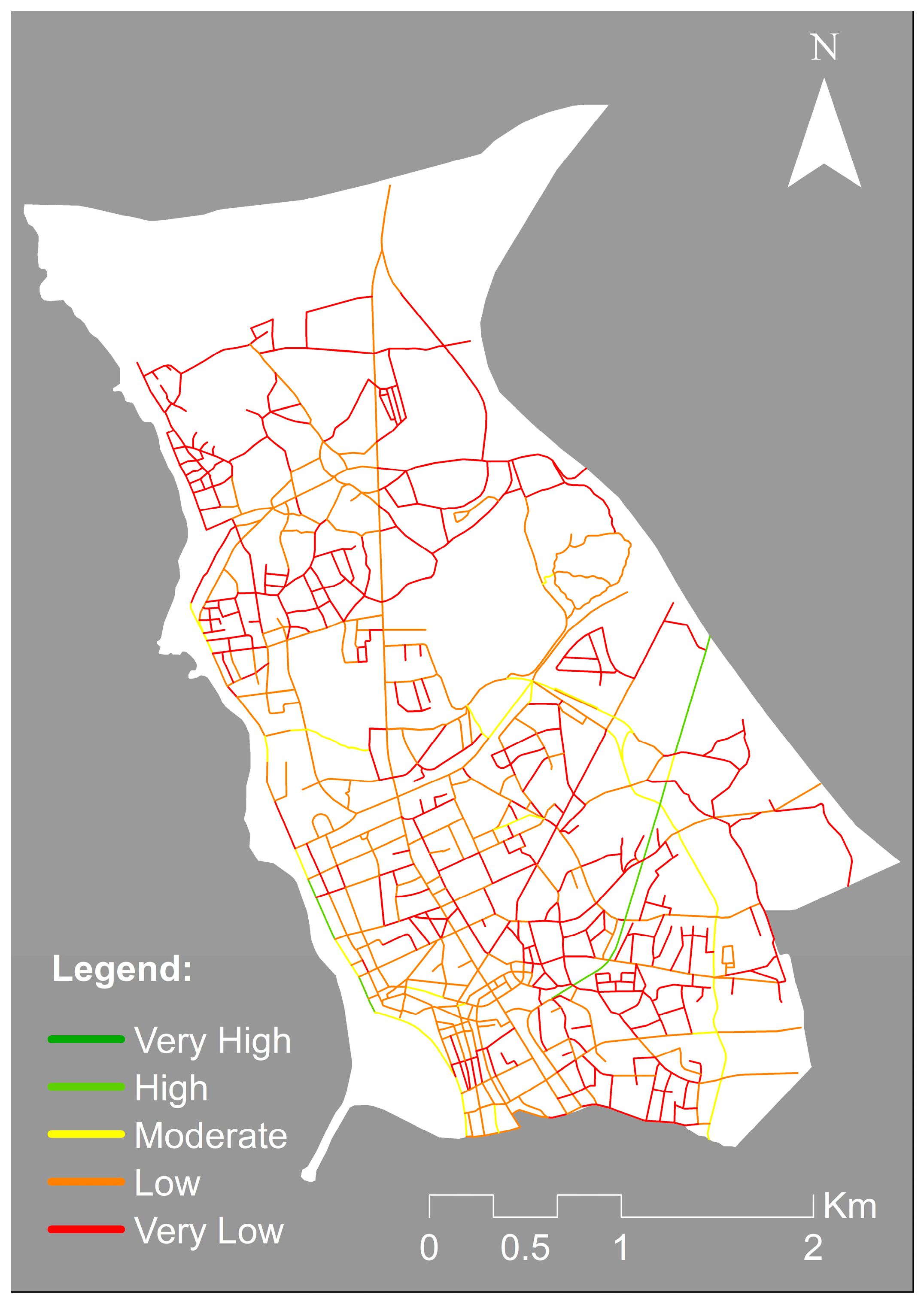
Table 8 depicts the accessibility of urban networks in the different zones. Data analysis reveals that Zones 6 and 7 have the lowest accessibility levels, with most segments classified as “Very Low” (78.9% and 78.4%, respectively). This observation is further supported by
Figure 5, where these zones are predominantly represented in red, indicating very low accessibility. Conversely, Zone 3 arises with a more balanced percentage across different levels, including 8.5% of segments classified as “Very High” accessibility. Zones 1, 2, 4, and 5 also exhibit a high proportion of segments with “Very Low” accessibility, but they also show some distribution within the “Moderate” and “High” levels, suggesting areas with better accessibility.
Table 9 provides data on cycling infrastructure across the different zones. An analysis reveals that most segments are classified as “Very Low” and “Low” in almost all zones, especially in Zones 6 and 7, where 65.8% and 71.8% of the segments, respectively, are at the “Very Low” level. Zones 1, 2, 3, and 4 also show significant percentages of segments with “Low” quality infrastructure, with Zone 1 presenting 72.9% of segments. Only a small fraction of Zones 5 and 3 have “Moderate” infrastructure, with 12% and 6.3% of segments, respectively.
Figure 6 visually confirms this trend, demonstrating a prevalence of red and orange colours, indicating “Very Low” and “Low” infrastructure across much of the network.
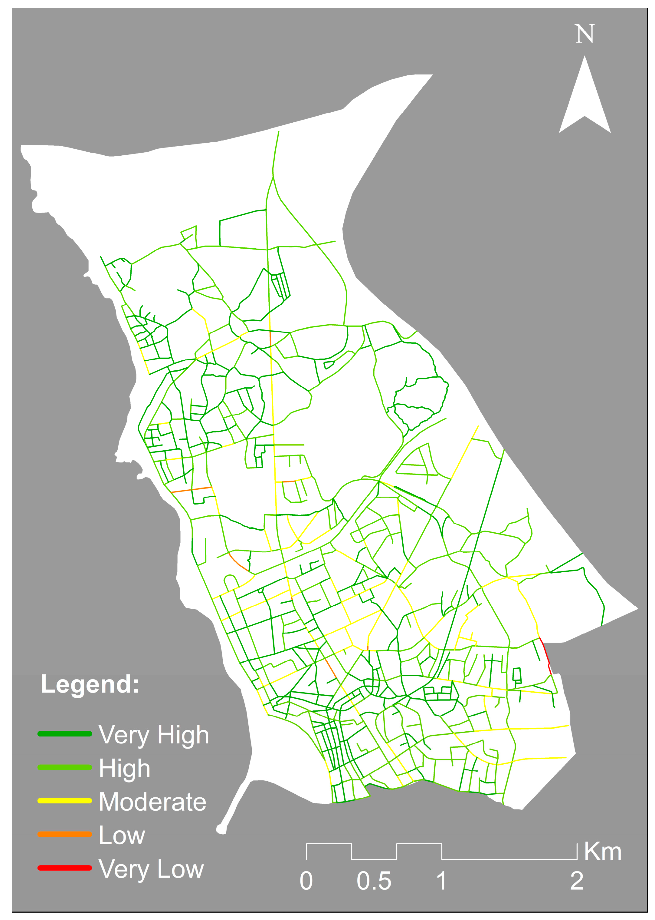
Table 10 depicts the findings on road features across the various analysed zones. Most zones have a high percentage of segments divided as “Very High” and “High.” Notably, Zones 7 and 2 stand out, with 63.4% and 57.9% of their segments falling under the “Very High” level, respectively. Zone 5 also demonstrates a substantial presence of segments with “High” road features (64.1%).
Figure 7 reinforces these results by illustrating a prevalence of green and yellow colours in the zones with the best road features, particularly in Zones 7, 2, and 5. In contrast, Zones 3 and 4, while containing a significant proportion of “Very High” and “High” segments, also comprise considerable percentages of “Moderate” segments. Overall, the data indicate that road features are largely favourable across most zones, particularly in Zones 7, 2, and 5.
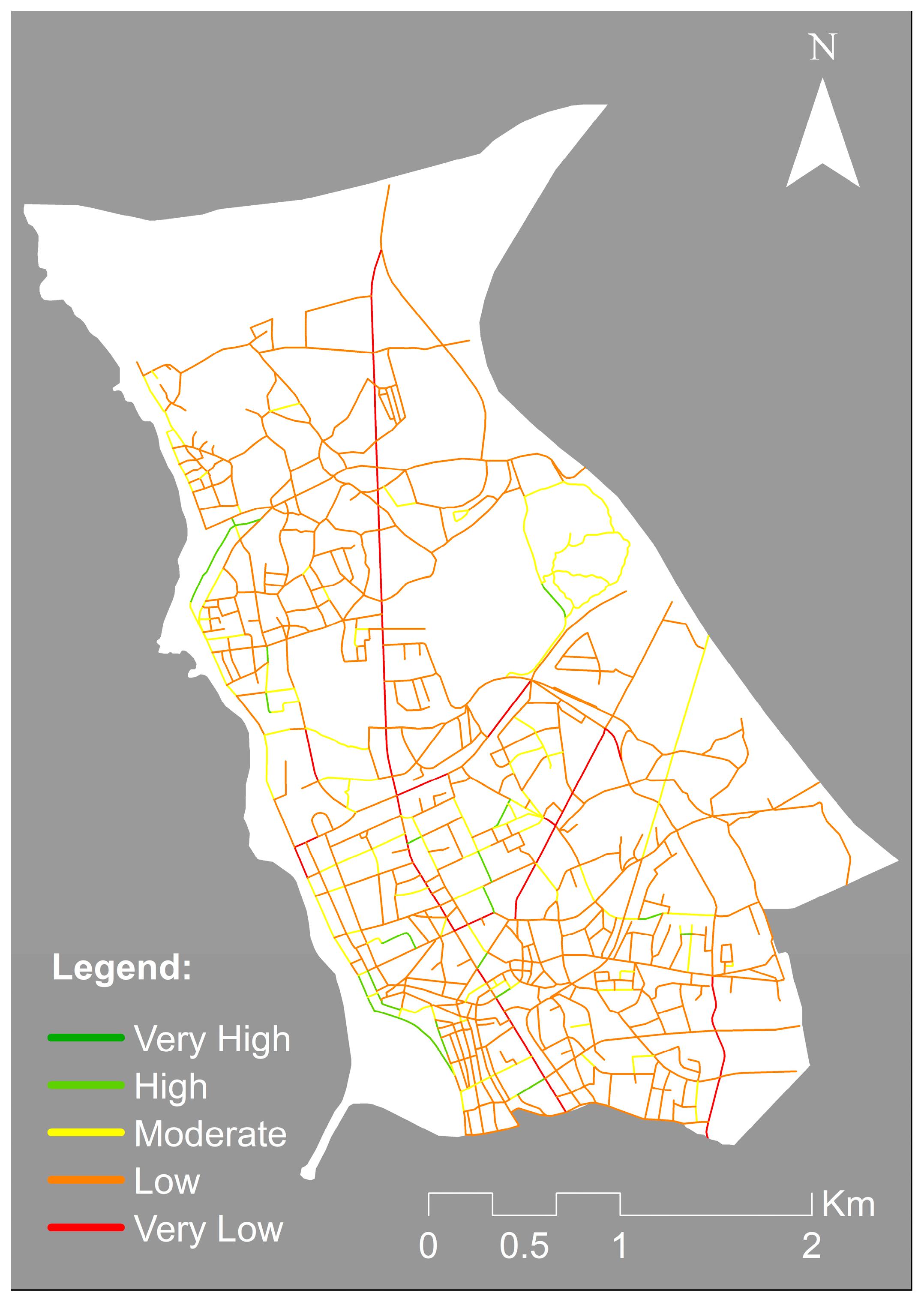
Table 11 displays the findings regarding the surrounding environment in the various analysed zones. Most segments in the studied zones are labelled as “Low” or “Very Low” in terms of the quality of the surrounding environment. Zones 5, 6, and 7 are notably concerning, with over 80% of segments classified as “Low” (83.3%, 88.2%, and 83.3%, respectively). While some zones have moderate percentages of “Moderate” segments, such as Zones 3 and 4, the prevalence of “Low” classifications is evident. This pattern is also observed in Zones 1 and 2, with 74.7% and 75.7% of segments classified as “Low”, respectively.
Figure 8 corroborates these findings, depicting an abundance of orange and red colours, representing “Low” and “Very Low” classifications. This underscores the need for substantial improvements in the surrounding environment of cycling infrastructures to create a more attractive network for users.
Table 12 provides data on cycling infrastructure safety across the different analysed zones. Zones 1 and 2 have most segments classified as “Very High” in safety (55.2% and 54.1%, respectively), indicating positive safety indicators. Zones 4 (43.2%) and 5 (44.1%) also show good safety levels. In contrast, Zone 3 shows more variation, with 35.6% of segments classified as “Moderate” and only 28.8% as “Very High”. Zones 6 and 7 have a considerable number of segments in the “High” and “Very High” levels, but also notable percentages of segments classified as “Moderate” or lower, particularly Zone 6, where 27.3% of segments are classified as “Low”.
Figure 9 confirms these observations, highlighting higher safety areas in green (very high) and lower safety areas in yellow (moderate) and red (very low). The central and western zones appear to have the safest infrastructure, while the peripheral zones, especially in the southeast, require improvements.
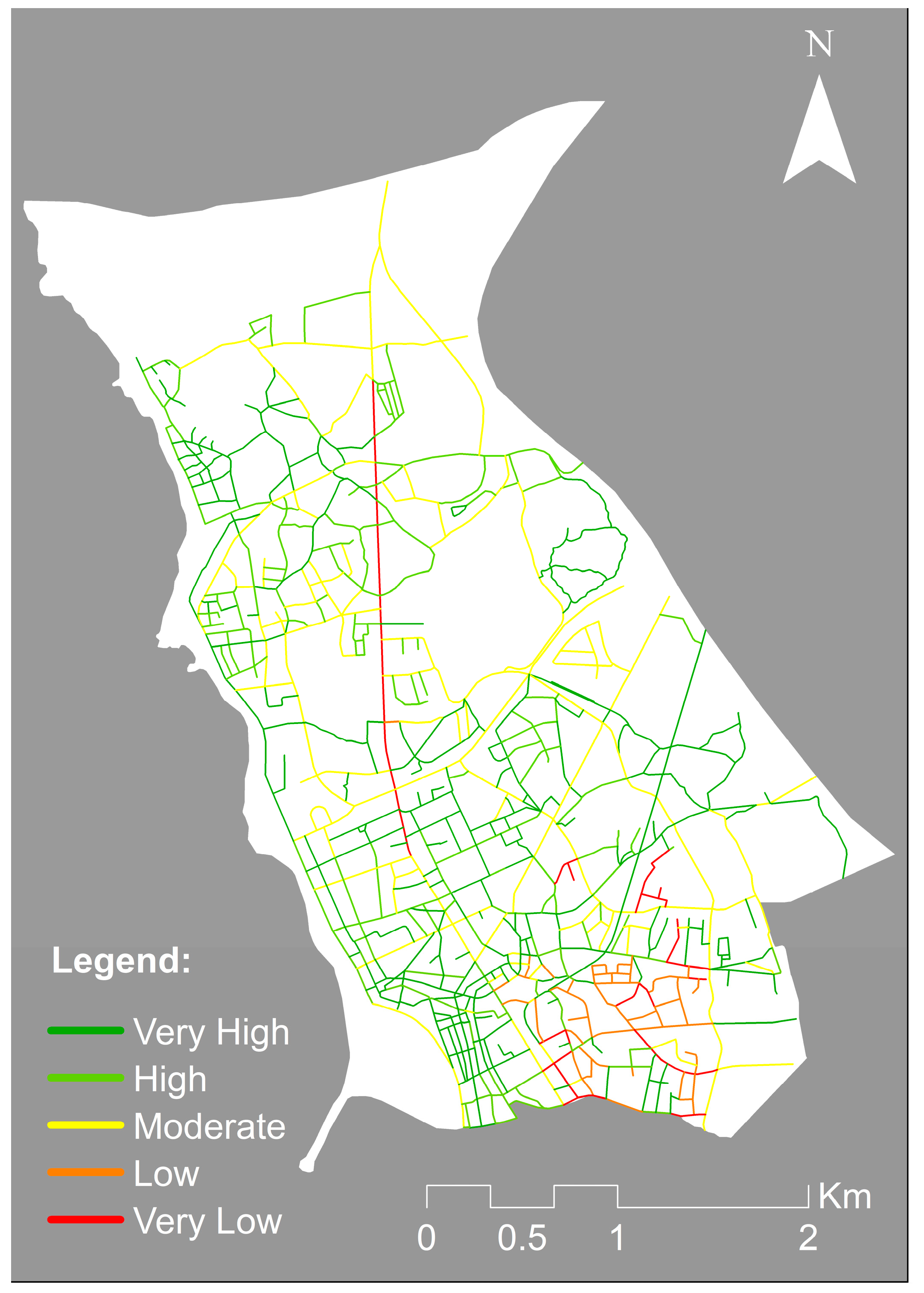
The “bikeability” index results are depicted in
Table 13, capturing the distribution of segments across different zones. Zones 1, 2, and 7 have achieved the highest “bikeability” scores, with most segments classified as “Moderate”. However, Zones 5 and 6 exhibit a higher proportion of segments classified as “Low”, indicating a need for improvement in these areas.
Figure 10 visually represents the data, highlighting that most zones, particularly in the central and northern areas, are classified as “Moderate” or “Low”. Few areas are classified as “High” or “Very High”, implying that while some zones possess high “bikeability”, challenges persist in making the entire cycling network more suitable. In summary, while Zones 1, 2, and 7 excel in “bikeability”, Zones 5 and 6 require significant enhancements to improve user cycling conditions.
4. Discussion
4.1. The Assessment of Criteria Influence
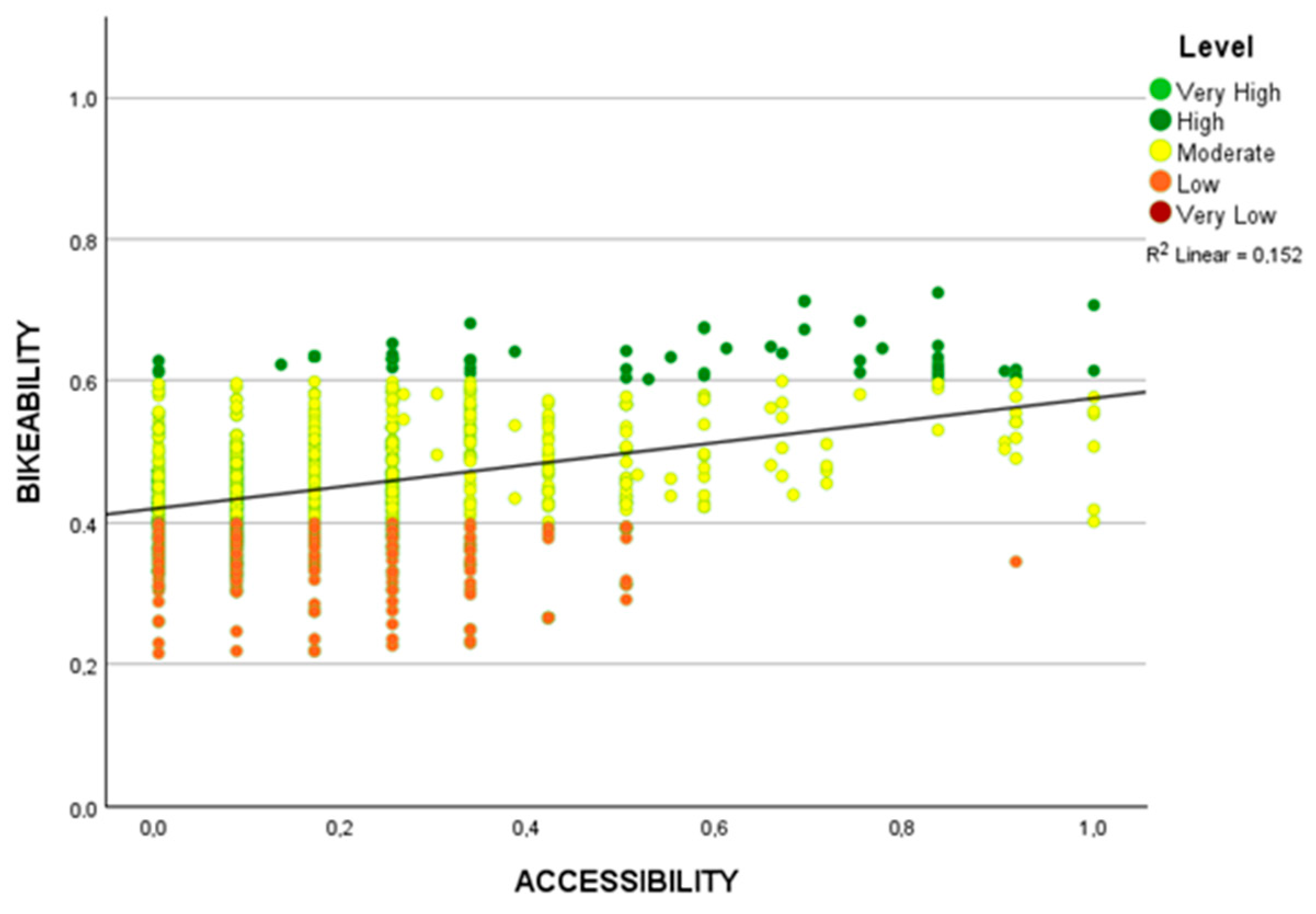
To understand how each of the five criteria affects Bikeability, we analysed scatter plots to examine the relationships between the values of each criterion and the bikeability index. These plots helped us identify trends, dispersion patterns, and correlations between the criteria and the final value of the index.
The analysis of
Figure 11 indicates a relatively weak relationship between Accessibility and Bikeability, with a coefficient of determination of R
2 = 0.152. The Accessibility criterion ranges from 0 to 1, with a higher concentration of data between 0.1 and 0.4. For lower levels of Accessibility, Bikeability tends to vary between low and moderate values. On the other hand, as Accessibility increases, there is a slight tendency for Bikeability levels to rise, with more frequent concentrations at higher levels. However, the relationship is not very pronounced, particularly between Accessibility values of 0 and 0.6, where the criterion does not appear to make a significant distinction in Bikeability behaviour. Despite a modest trend of increasing Bikeability with higher levels of Accessibility, this criterion alone is not a strong indicator of the bikeability index, as different levels of Bikeability can be observed across a wide range of Accessibility values.
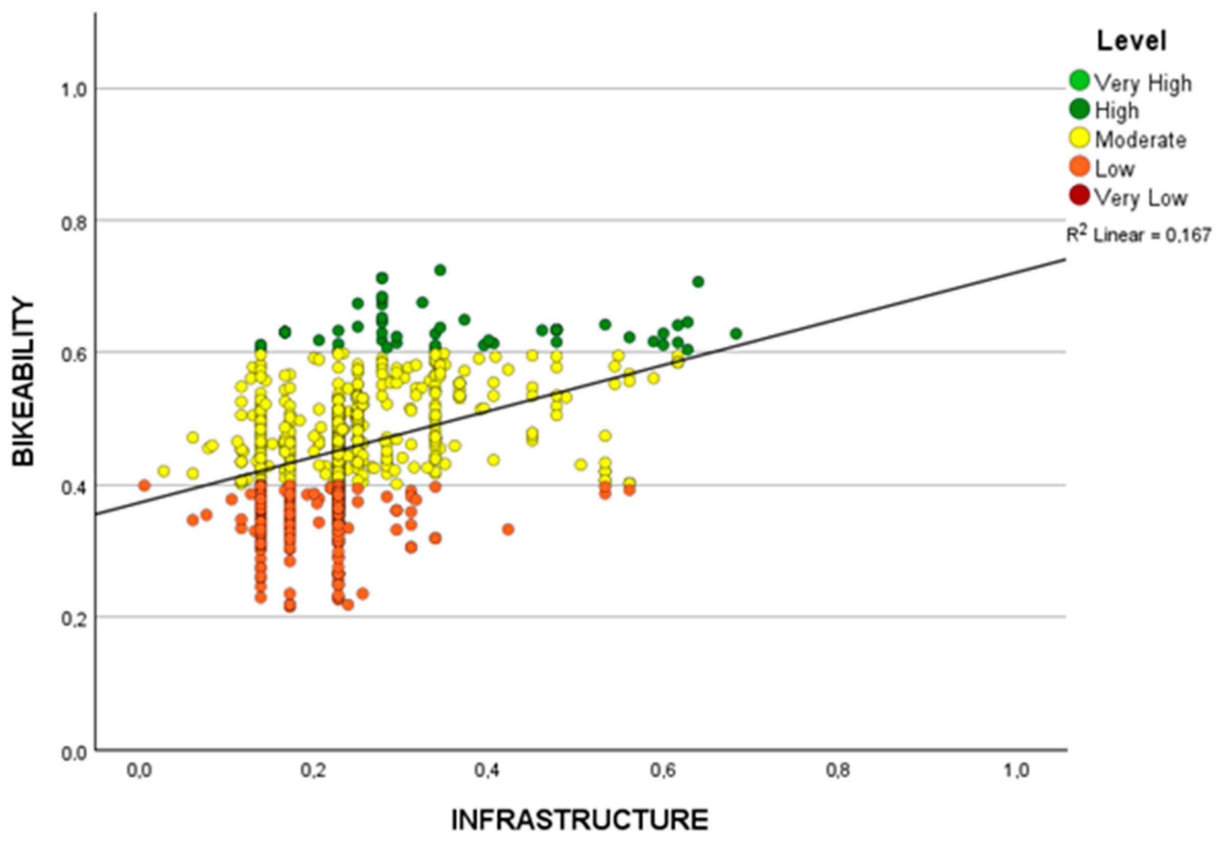
Figure 12 illustrates that the Infrastructure score ranges from 0 to 1, with the highest concentration between 0.1 and 0.4. Lower Infrastructure scores are mainly associated with “Low” and “Moderate” Bikeability, while scores above 0.4 tend to be concentrated in “Moderate” and “High” Bikeability. Although there is a positive relationship between Infrastructure and Bikeability, with a tendency for Bikeability to increase as Infrastructure improves, the coefficient of determination R
2 = 0.167 indicates that this correlation is not particularly strong.
High Bikeability values are observed at different levels of Infrastructure, suggesting that while the criterion is relevant, it is not sufficient to explain the bikeability index. Therefore, it is concluded that Infrastructure contributes to Bikeability, but other factors play an important role in its determination.
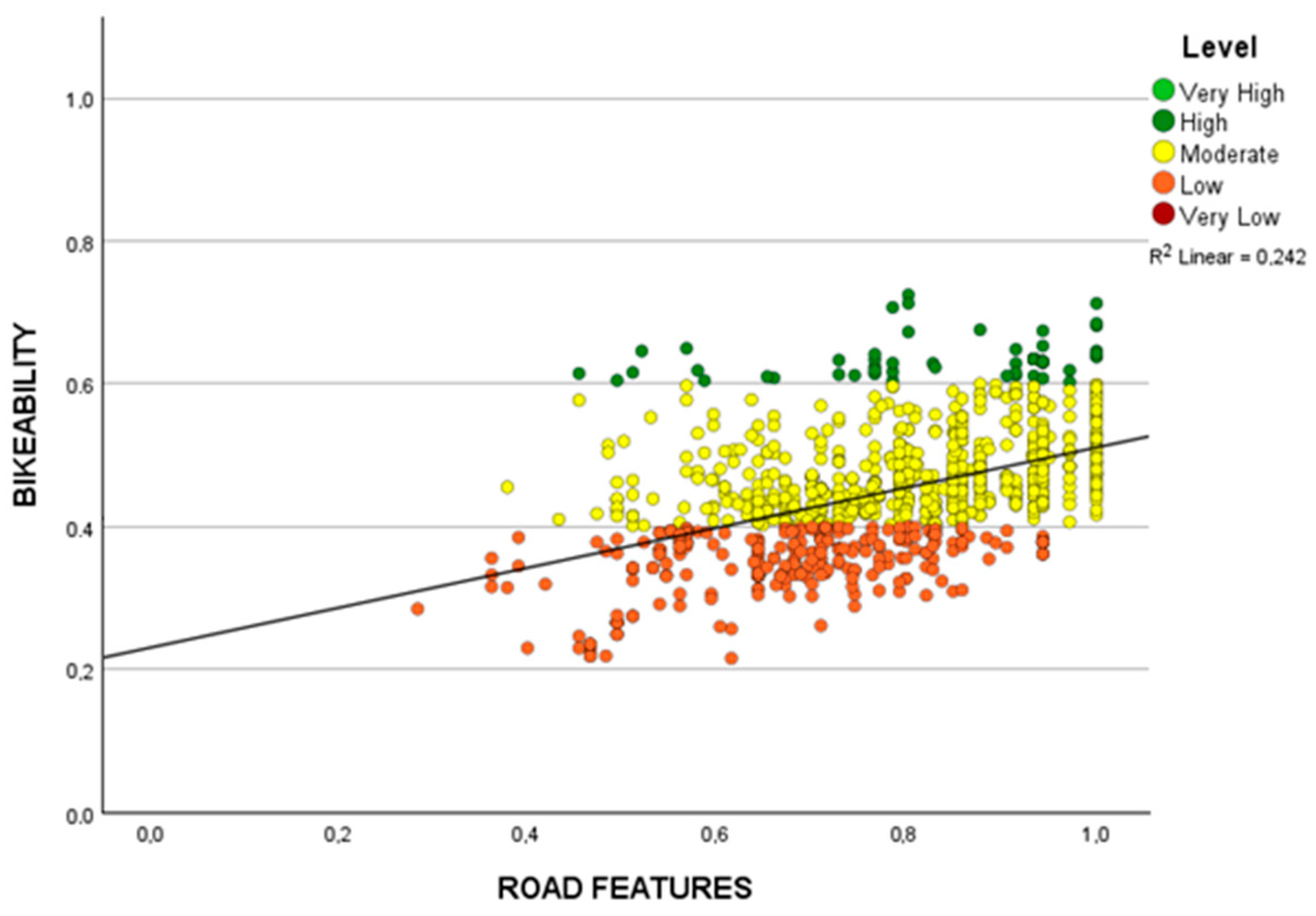
Figure 13 depicts a noticeable correlation between the Road Features criterion and Bikeability, with a coefficient of determination of R
2 = 0.242, indicating a moderate association. The values for this criterion range from 0 to 1, and there is a discernible trend of increasing Bikeability as Road Features values rise. This trend persists despite the presence of different Bikeability levels across various values of the criterion.
At lower levels of Road Features (between 0 and 0.4), the majority of cases are concentrated in the lower Bikeability levels, indicating a strong association between lower quality or quantity of road characteristics and low Bikeability. Conversely, as Road Features values increase, there is a more evident trend towards higher Bikeability, with a greater concentration of moderate values, high values, and values above 0.6. This relationship suggests that the Road Features criterion is a reliable indicator for Bikeability, especially at higher levels, where there is a clearer distinction between the different Bikeability categories, with a notable separation between low and high Road Features values.
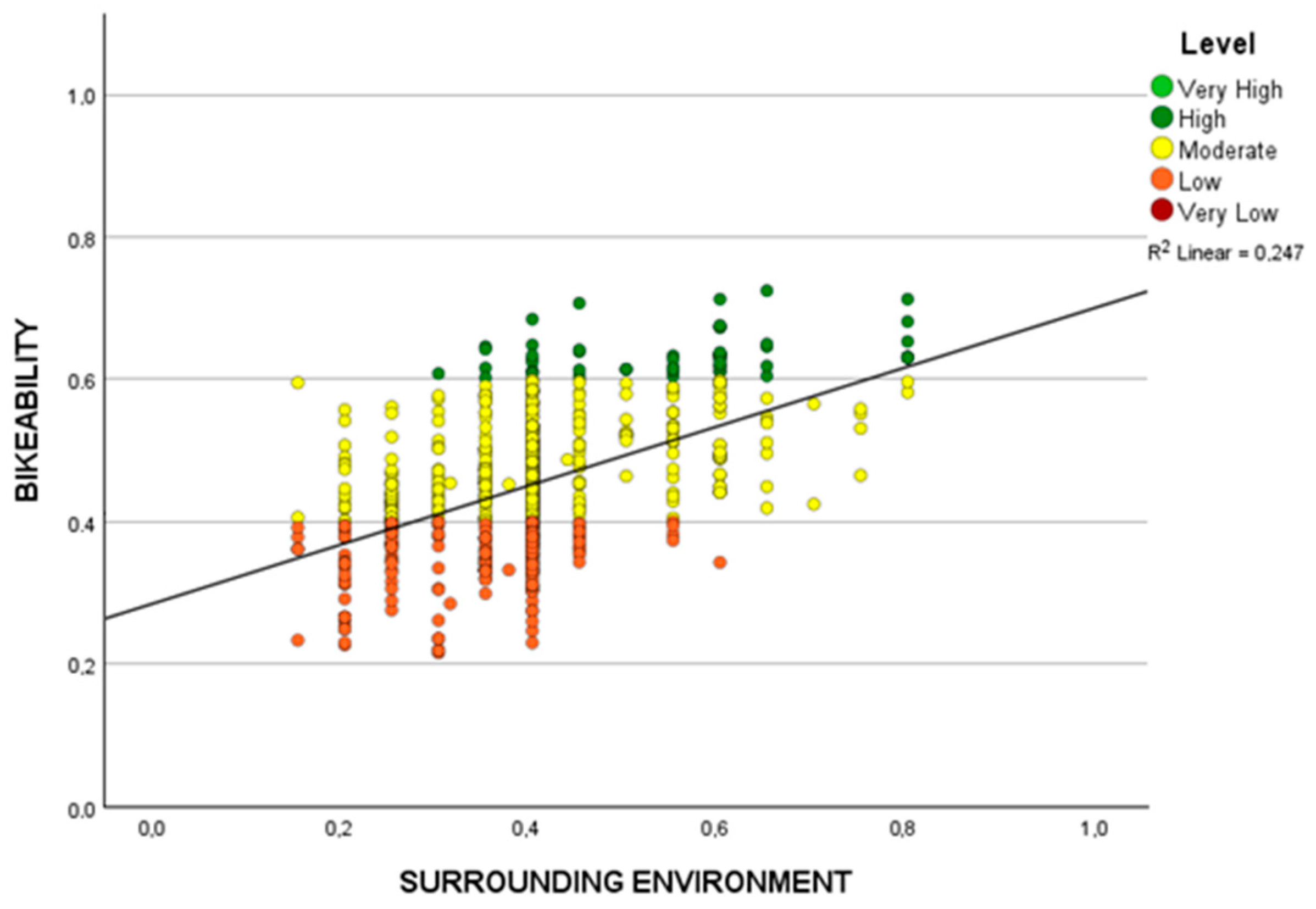
The data in
Figure 14 illustrate a moderate correlation between Surrounding Environment and Bikeability (R
2 = 0.247), suggesting that as the surrounding environment improves, bikeability tends to increase. When the Surrounding Environment value is low (below 0.4), Bikeability is limited to low and moderate levels. However, when the Surrounding Environment value is 0.4 or higher, an increase in moderate and high Bikeability levels becomes evident. The variability in Bikeability levels across different ranges of Surrounding Environment is significant, indicating that while improvements in the surrounding environment generally enhance bikeability, there are still instances of high Bikeability in less favourable environments. In summary, the Surrounding Environment positively influences Bikeability, especially for values above 0.4. However, there are exceptions where high Bikeability levels occur, even with lower scores in this criterion.
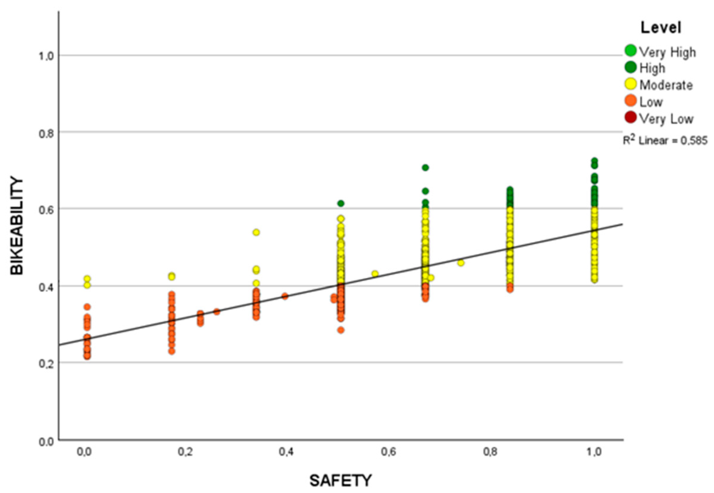
The analysis of
Figure 15 reveals a relatively strong correlation between Safety and Bikeability (R
2 = 0.585), indicating that an increase in safety is associated with an increase in bikeability. For low Safety values (between 0 and 0.4), low Bikeability levels are predominant. As the level of Safety increases, Bikeability also improves significantly, with a more significant presence of high Bikeability levels for scores above 0.6 in the Safety criterion. The pattern is clear: low Safety values correspond to low Bikeability levels, and vice versa. Although there are instances of moderate and even high Bikeability at lower Safety levels, the highest concentrations of high Bikeability levels are associated with higher Safety values. In summary, the Safety criterion strongly influences Bikeability, demonstrating a clear improvement relationship as safety increases.
The scatter plot analysis shows that all criteria significantly contribute to the Bikeability despite varying relationships. Safety has the strongest correlation, indicating that as safety values increase, bikeability levels also rise. Road Features and Surrounding Environment also have moderate positive correlations, while Infrastructure and Accessibility show weaker correlations than expected. This could be due to the limited segregated cycling infrastructure in relation to the road network and the lack of integration between cycling and public transport in internal journeys. These criteria may have a more restricted impact in this specific analysis, but they should not be underestimated. High bikeability was seen in safety, road features, and surrounding environment but was less clear for infrastructure and accessibility. This variation suggests the analysed variables have interesting discretionary value, reinforcing the relevance of the chosen criteria. The lack of a fully linear relationship between the criteria and the bikeability index highlights the need to adjust the weights of these criteria with stakeholder participation in future analyses to reflect local priorities in cycling planning.
4.2. Póvoa de Varzim’s Network Bikeability
The approach used in this study expanded the traditional criteria for developing a bikeability index that shares the characteristics of two prominent methodological families. It not only incorporated environmental aspects related to air quality and noise but also variables for multimodality and parking facilities. This allowed for a comprehensive analysis of the same features’ positive and negative aspects. For instance, while trees and vegetation along a pathway can provide shade and a pleasant environment for cyclists, they can also increase the risk due to the accumulation of dry leaves and high pollen levels. Similarly, a region with many destinations may be less appealing if there are inadequate connections between public transport and bicycles [
56,
57]. Moreover, defining a comprehensive set of parking variables alongside linear infrastructure offers detailed insights that are crucial for transportation planning. This integrated approach ensures that multiple aspects of parking are considered, enhancing the effectiveness and accuracy of planning efforts.
The results analysis yields valuable insights into the urban network within the study region and its cycling potential. These insights have practical implications for urban planning and transportation development. When analysing accessibility, we found that while there are differences between zones, accessibility generally follows a pattern linked to proximity to the coast and main axes. This finding can guide the placement of future transportation facilities and the development of cycling infrastructure. Additionally, we observed that most bus stops lack bicycle parking or regulations permitting bicycles to board buses. This underscores the need for improved multimodal interfaces, a key area for future development. After assessing infrastructure, it becomes evident that significant challenges must be addressed. Although there is evidence of a cycling network, it primarily consists of painted linear infrastructure (
Figure 1b) and isolated portions with varying degrees of separation. The same applies to the few protected intersections scattered throughout the network. Concerning the cross-section, while the widths of the linear infrastructures satisfy the considered standards, buffer space is absent in sections with some level of separation (
Figure 1b).
The availability and quality of bicycle parking spaces are essential for promoting cycling as a mode of transportation [
58]. This aspect is the main critical point in the cycling network of the study area. The bicycle parking facilities are relatively basic, consisting mainly of bike racks (
Figure 1b), and are often unprotected, blending into the urban surroundings. The presence of fly-parking in busy areas raises the possibility of increasing the number of spaces in these regions and making them more visible. It is noted that very few bicycle parking spaces in the study area have accessible toilets or changing rooms. Adequate bicycle parking facilities can encourage more people to adopt cycling as a sustainable transportation option. It is also crucial to ensure that bicycle parking spaces are easily accessible and visible, instilling a sense of security among cyclists when they park their bicycles [
58].
When analysing urban infrastructure characteristics, it is important to consider how topography affects mobility [
35,
40]. Luckily, the target area does not have to worry about slope, as the urban area of Póvoa de Varzim is in a coastal region with appropriately sloped urban segments. Additionally, it is essential to note that road surface quality plays a significant role in ensuring a safe and comfortable travel experience. Irregularities in road surfaces can be a challenge for active modes of transportation [
47]. In the study area, the historic region has a higher incidence of segments with significant irregularity (cobblestone). Meanwhile, surfaces of more regular materials like concrete or asphalt can be found on the main axes. However, more surface irregularities like cracks, fissures, and potholes occur farther from the central area and axes.
The evaluation of road features considers various characteristics that align with the existing road hierarchy. Segments of the main axes score lower than those that do not compose an axis. Irregular parking is a typical street issue, often leading to traffic conflicts. The layout of bus stops also adds to the problem, as most intersect with the road during passenger boarding and exiting. The tree typology is acceptable; although there are a few with a higher pollen level, they are scarce. Evaluating bodies of water and parks aligns with expectations, with areas near coastal regions, squares, and the city park receiving higher scores. After analysing the surroundings and traffic criteria, it was found that the road hierarchy behaviour in the study area also repeats for the traffic criterion. This can be observed in the segments that make up the main axes. The similarity between the resulting maps of the two criteria suggests a strong connection between traffic intensity and noise levels. This finding is consistent with the results of other studies [
59].
The methodology, encompassing comprehensive criteria and a systematic and detailed process of data collection and processing for variables, offers a holistic view of cycling potential. This comprehensive approach benefits engineers, urban planners, and municipalities. It aids in their understanding of how the cycling potential of an urban network is influenced by a wide range of built environment aspects, with physical infrastructures remaining crucial. This knowledge can then be used to develop guidelines and action plans by examining isolated aspects through partial results by criterion or by considering the synergistic relationship of factors, as substantiated in this bikeability index.
Although some of the indicators employed in this study are more closely related to destination attractiveness, they were retained due to the holistic approach adopted, which considers the urban network as a whole. This approach aims to capture the complexity of transportation systems, including factors that influence not only routes but also the accessibility and convenience of destinations. While we acknowledge the clear differences between route and destination attractiveness and that the relatively small study area may not fully reflect the need for intermodal transfers or destination amenities such as bicycle parking at bus stops or toilet and shower facilities, we chose to retain these variables to reflect the reality of larger urban cycling networks where such factors may play a key role in transportation choices. The inclusion of these elements also reflects the intention to make the model applicable to larger areas in future studies. However, we agree that a more focused discussion on the distinction between routes and destinations is necessary. One limitation of this study is that, due to the reduced scale of the study area, indicators more relevant for larger areas, such as intermodal opportunities, may have limited applicability. In the context of this study, we maintained the accessibility and amenities indicators as part of the segmented analysis of the urban network. For future research, destination-based metrics calculated over larger areas may provide a more accurate and context-sensitive picture of urban bikeability.
5. Conclusions
Providing a cycling network infrastructure is crucial to fostering cycling as a regular transportation mode and achieving high bicycle usage levels. This paper introduces a novel approach to measuring urban network bikeability, expanding the standard cycling infrastructures, safety, and accessibility approach to encompass six critical factors, namely accessibility, linear infrastructure, parking infrastructure, road features, surrounding environment, and traffic. This innovative framework not only aids understanding of how the cycling potential of an urban network is influenced by a wide range of built environment aspects but also reveals the importance of these factors. The primary objective of this paper is to present a practical approach, followed by “how-to-do” measures, to assess bikeability based on GIS methodologies. The target area for testing the bikeability assessment was the central region of Póvoa de Varzim, located in the Porto Metropolitan Area in the northern region of Portugal.
The analysis concluded that the chosen set of variables to assess the bikeability index was appropriate. While there is a general trend of an increasing bikeability index as the values of the criteria rise, a clear and uniform trend for all criteria could not be identified. This suggests that the variables have a relevant discriminatory capacity, allowing for identifying different bikeability levels across a diverse range of criteria values. The current model lacks weights for each criterion or variable, which is a significant limitation. Future work will involve stakeholders assigning appropriate weights to each criterion to enable a more robust evaluation of the bikeability index, adjusting the relative impact of each variable based on local context and stakeholder priorities. To strengthen the model’s robustness, we recommend collecting utilisation data to assess the correlation between the bikeability index and actual cyclist usage. Additionally, surveys on cyclists’ preferences could shed light on how the variables in this study influence bikeability. These steps, although challenging in a developing cycling city, are vital for validating the metrics and improving the model. Due to the complex relationships between the factors, the simple correlation between the bikeability index and the criteria may not offer a conclusive or sufficient statistical analysis. A more comprehensive approach must be adopted to improve the model by integrating the indicators identified in the existing research with the actual conditions of the study area. In essence, assigning weights based on stakeholder participation will be crucial for refining the model, making it more precise and applicable in various contexts.
When looking at the overall results of the bikeability index, it is clear that most of the study area network scores fall between 0.30 (low) and 0.50 (moderate). The majority of the central zones and some coastal areas are classified as “Moderate” (in yellow), indicating areas that could be improved. Zones with a “Low” classification (in orange) are scattered throughout various parts of the city, especially in the outskirts and areas further from the central urban core, highlighting areas for potential intervention. No segments were identified with “Very High” bikeability, and only a tiny fraction exhibited “Very Low” bikeability. This approach makes a significant contribution by addressing factors often overlooked in bikeability indexes, such as the availability, type, and features of bicycle parking facilities, as well as environmental aspects like noise and pollen levels. The methodology stands out for its comprehensive evaluation of parameters, making it both easy to implement and adaptable to diverse situations. It is particularly beneficial for cities like Póvoa de Varzim, which are committed to promoting cycling and reducing car dependency by developing appropriate infrastructure for regular bicycle use.
Furthermore, considering the emerging phenomena in cycling—such as electric bicycles—it is essential to consider that these technological advances can reduce the relevance of criteria such as slope and accessibility due to electric assistance while raising the need for specific infrastructure, such as charging stations. Developing a new index that considers the distinction between conventional and electric bicycles may be necessary to reflect these changes. Additionally, integrating these modes of transport and sharing systems needs to be considered to adjust the index to urban mobility’s current and future realities. This new index could help capture technological particularities and ensure that bikeability analysis remains relevant, with stakeholder participation being essential in defining and weighting these new criteria.


