
Influence of Technical Reasons on Cost Overruns of Infrastructural Projects: A Sustainable Development Perspective


Abstract
1. Introduction
2. Materials and Methods
Samples Editing
3. Results
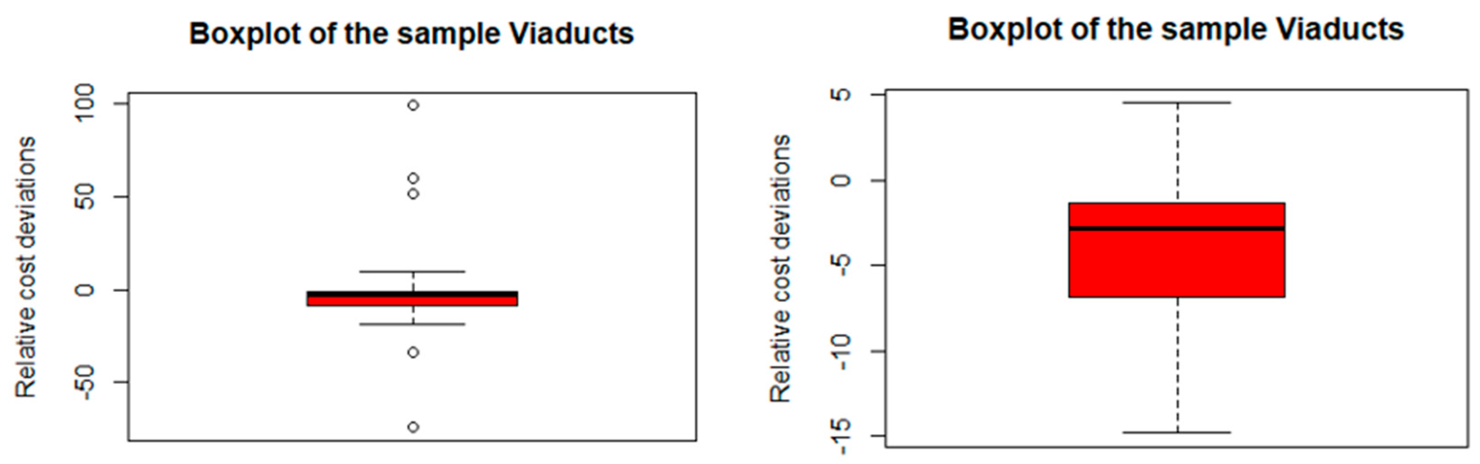
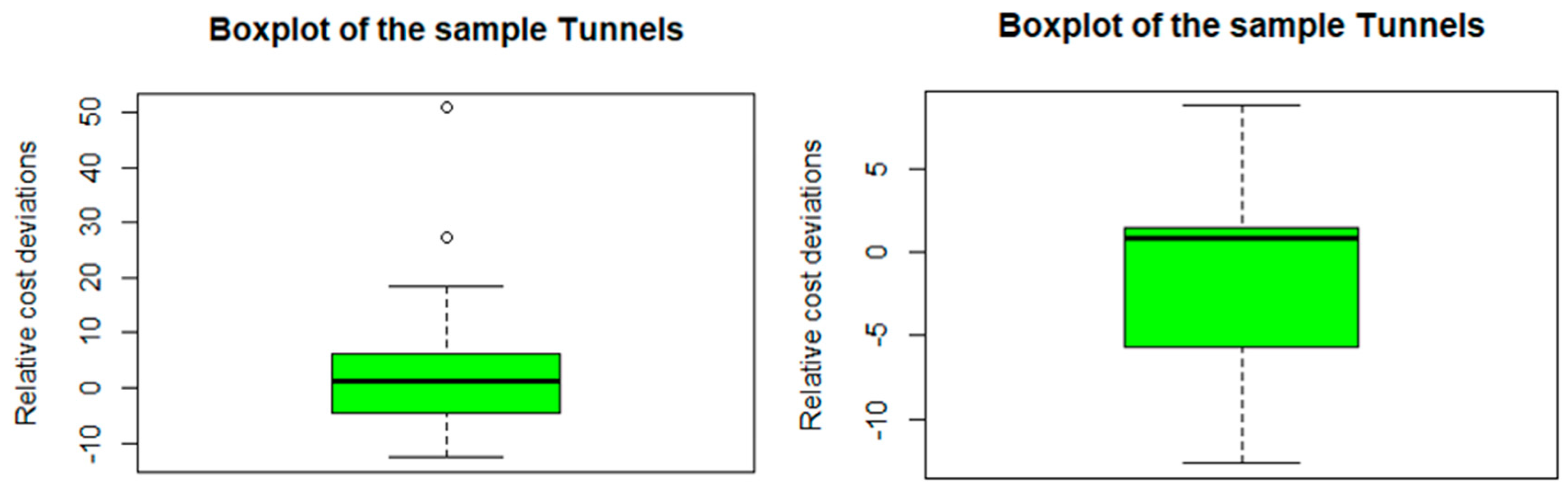
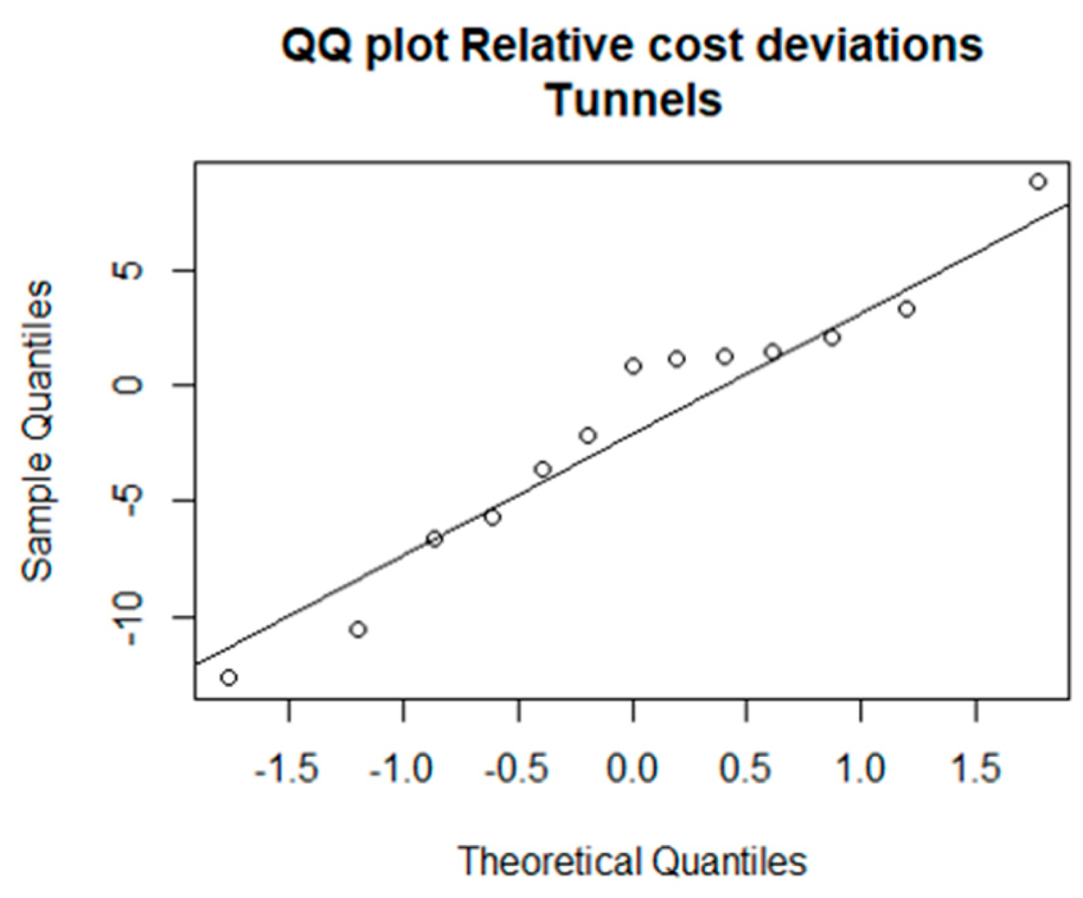
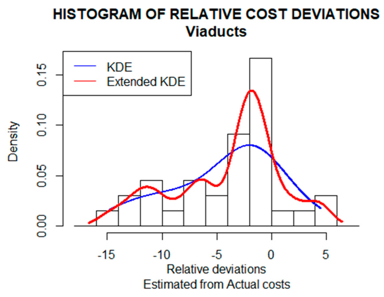
3.1. The Nature of the Random Variable
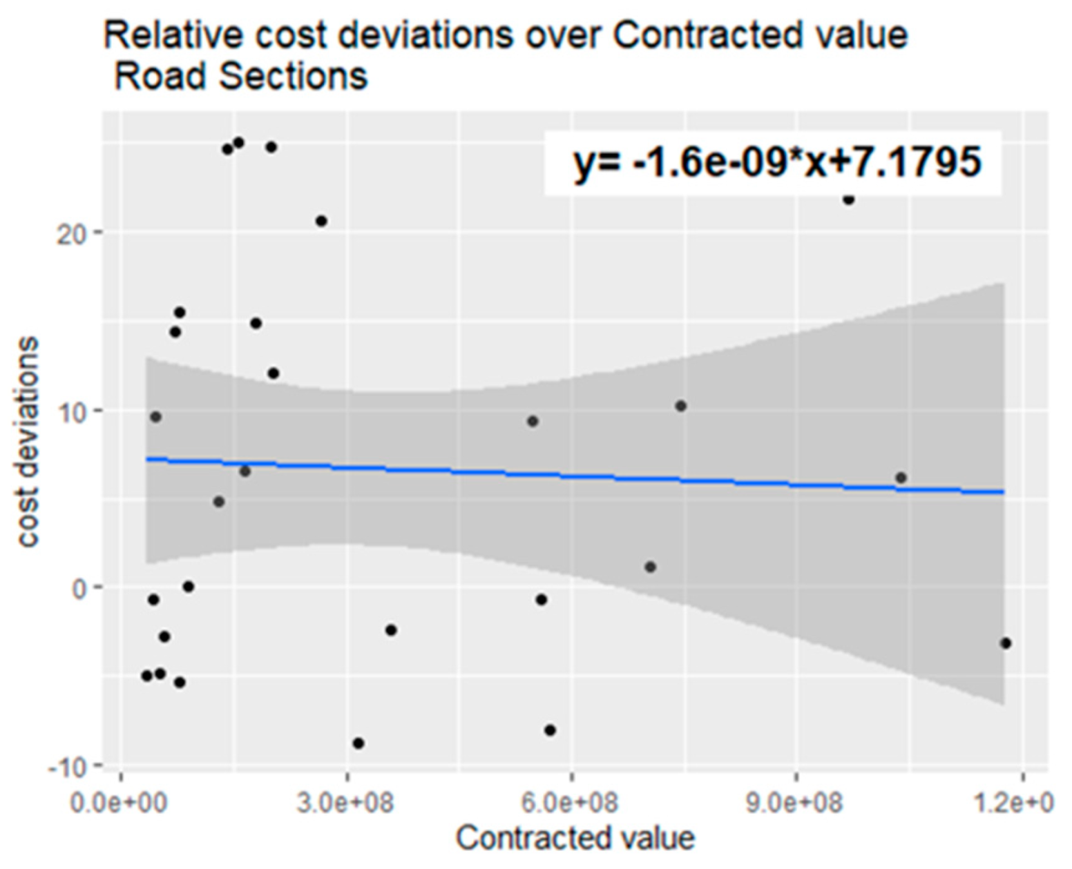
3.2. Results of Normalizing Classes by the Ratio of Contract Value to Cost Deviations
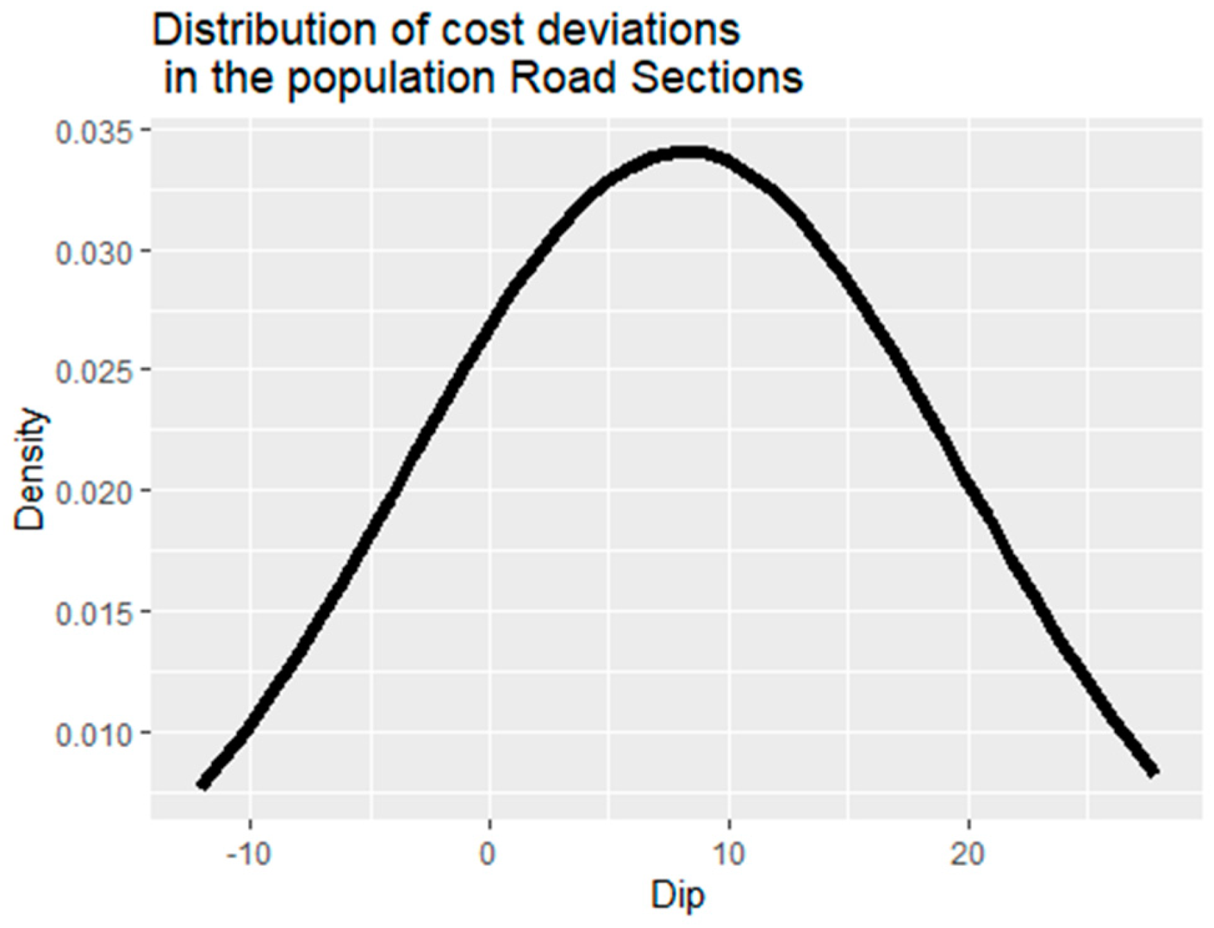
3.3. Statistical Characteristics of Discrepancies Between the Actual and Contractually Agreed Costs
4. Discussion
5. Conclusions
Author Contributions
Funding
Institutional Review Board Statement
Informed Consent Statement
Data Availability Statement
Conflicts of Interest
Appendix A

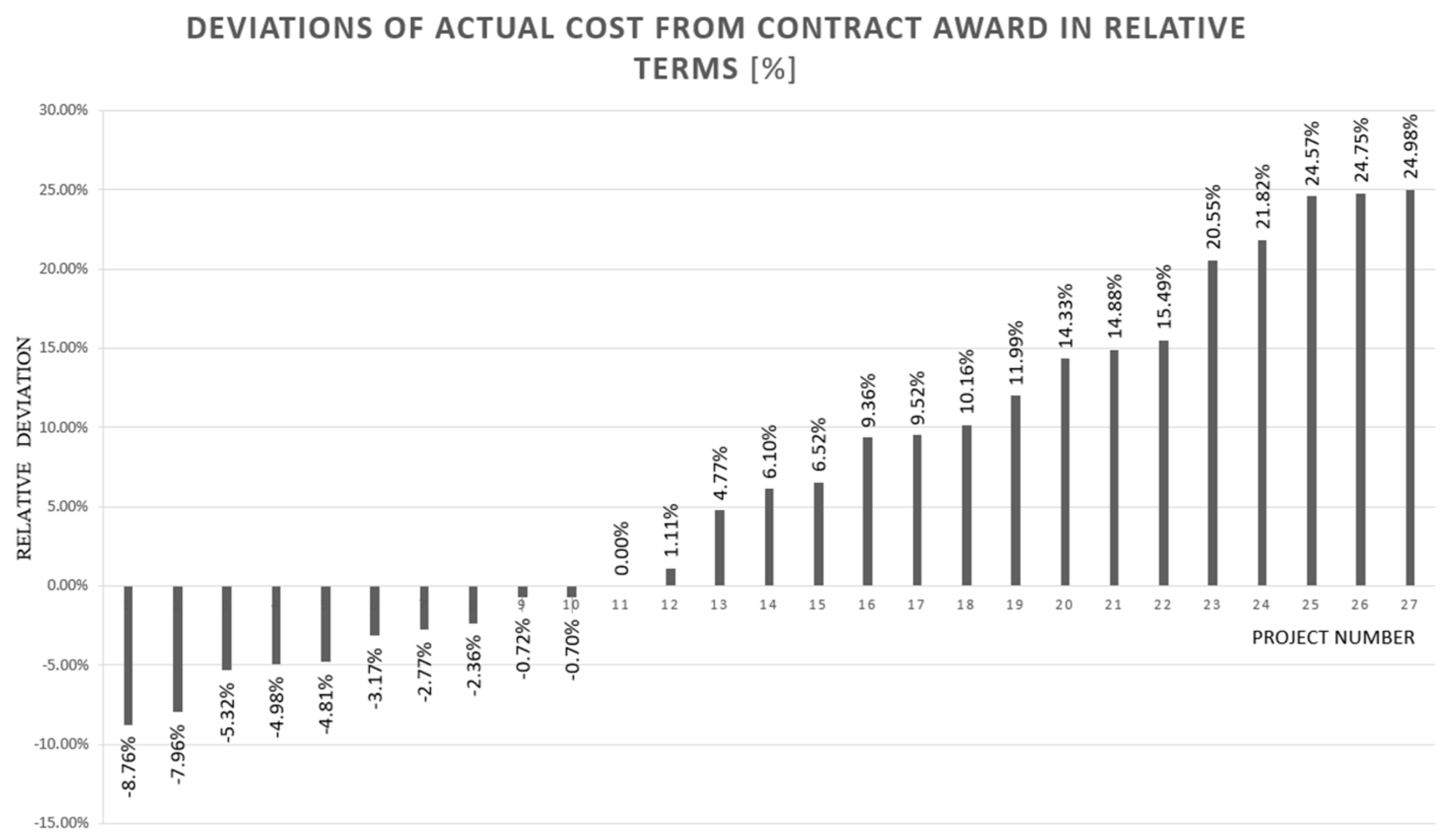
| No. | SECTIONS | Contractually Agreed Costs (TContr) | Final Costs (TFin) | Relative Cost Deviation (TContr − TFin)/TContr |
|---|---|---|---|---|
| 1 | Čvor Sv. Rok—tunel Sv. Rok | 20,632,526.67 €Eur | 25,786,531.85 €Eur | 0.2498 |
| 2 | Tunel Sv. Rok—Maslinica | 26,364,944.93 €Eur | 32,891,254.26 €Eur | 0.2475 |
| 3 | Maslinica—Zadar 1 | 11,849,363.43 €Eur | 11,849,363.43 €Eur | 0 |
| 4 | Zadar 1—Zadar 2 | 9,733,622.39 €Eur | 11,128,867.00 €Eur | 0.1433 |
| 5 | Zadar 2—Benkovac | 17,302,716.,30 €Eur | 18,128,062.88 €Eur | 0.0477 |
| 6 | Benkovac—Pirovac | 23,965,583.96 €Eur | 27,532,802.97 €Eur | 0.1488 |
| 7 | Pirovac—Skradin | 10,236,890.31 €Eur | 11,822,927.87 €Eur | 0.1549 |
| 8 | Skradin—Šibenik | 18,912,329.26 €Eur | 23,558,525.77 €Eur | 0.2457 |
| 9 | Šibenik—Vrpolje | 21,892,760.42 €Eur | 23,319,323.76 €Eur | 0.0652 |
| 10 | Prgomet—Dugopolje | 35,514,005.82 €Eur | 42,812,117.55 €Eur | 0.2055 |
| 11 | Dugopolje—Bisko | 72,869,393.,20 €Eur | 79,687,235.37 €Eur | 0.0936 |
| 12 | Bisko—Šestanovac | 137,771,.341.79 €Eur | 146,174,528.21 €Eur | 0.061 |
| 13 | Šestanovac—Zagvozd | 93,392,.451.,41 €Eur | 94,427,796.05 €Eur | 0.0111 |
| 14 | Zagvozd—Ravča | 128,658,460.,96 €Eur | 156,732,160.31 €Eur | 0.2182 |
| 15 | Čvor Ploče—Luka Ploče | 98,680,769.14 €Eur | 108,708,836.74 €Eur | 0.1016 |
| 16 | Spojna za grad i luku Ploče | 7,551,553.54 €Eur | 7,342,490.94 €Eur | −0.0277 |
| 17 | Čvor Ploče—granica BiH | 6,855,725.36 €Eur | 6,525,857.44 €Eur | −0.0481 |
| 18 | Spojna cesta i tunel Sv. Ilija | 41,987,604.48 €Eur | 38,307,961.73 €Eur | −0.0876 |
| 19 | Zabok—Krapina, 1. dio | 5,799,559.62 €Eur | 5,758,836.45 €Eur | −0.007 |
| 20 | Zlatar Bistr.—Andreševac, 1. faza | 4,504,239.51 €Eur | 4,279,732.59 €Eur | −0.0498 |
| 21 | Zlatar Bistr.—Andreševac, 2. faza | 10,515,896.19 €Eur | 9,956,165.61 €Eur | −0.0532 |
| 22 | Dubovo—Kapja | 5,994,243.31 €Eur | 6,564,939.57 €Eur | 0.0952 |
| 23 | Sredanci—Đakovo | 74,296,614.63 €Eur | 73,762,642.00 €Eur | −0.0072 |
| 24 | Osijek—Đakovo | 156,374,043.98 €Eur | 151,413,514.31 €Eur | −0.0317 |
| 25 | Jakuševac—V. Gorica, 0–6,3 km | 75,774,286.13 €Eur | 69,743,224.39 €Eur | −0.0796 |
| 26 | Jakuševac—V. Gorica, 6,3–8,4 km | 26,796,178.51 €Eur | 30,009,197.24 €Eur | 0.1199 |
| 27 | Buševec—Lekenik | 47,840,327.92 €Eur | 46,710,938.79 €Eur | −0.0236 |
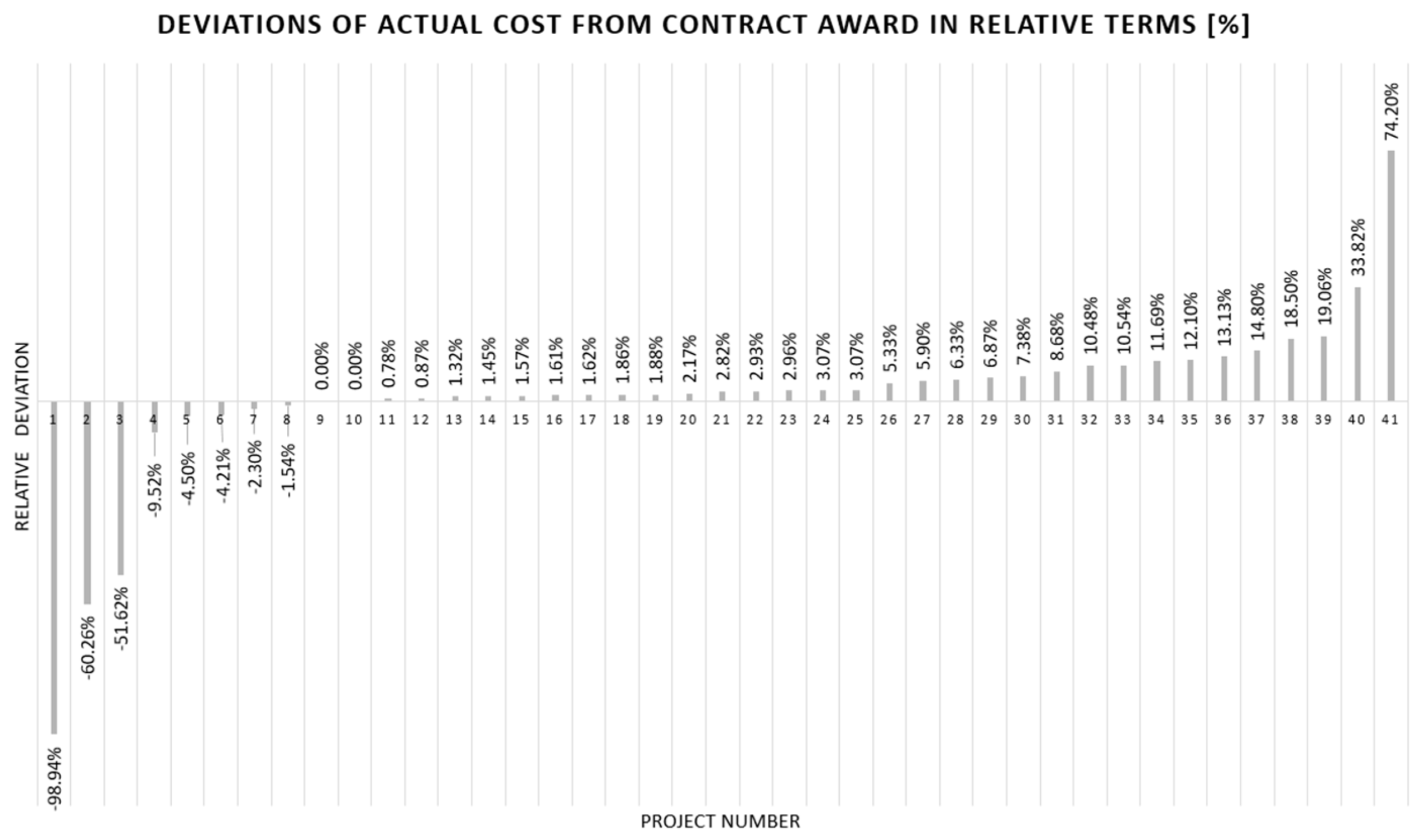
| No. | VIADUCTS | Contractually Agreed Costs (TContr) | Final Costs (TFin) | Relative Cost Deviation (TContr − TFin)/TContr |
|---|---|---|---|---|
| 1 | Krpani | 3,012,643.36 €Eur | 3,570,079.16 €Eur | −0.185 |
| 2 | T. Sv. Rok—Maslinica (objekti) | 18,693,745.28 €Eur | 18,996,450.24 €Eur | −0.0162 |
| 3 | Maslinica—Zadar 1 (prolazi) | 3,418,518.37 €Eur | 4,574,522.26 €Eur | −0.3382 |
| 4 | Zadar 1—Zadar 2 (objekti) | 1,023,981.90 €Eur | 1,147,862.55 €Eur | −0.121 |
| 5 | Zadar 1—Zadar 2 (prijelazi) | 1,068,784.68 €Eur | 1,861,841.56 €Eur | −0.742 |
| 6 | Zadar 2—Benkovac (objekti) | 5,376,048.35 €Eur | 5,376,048.35 €Eur | 0 |
| 7 | Zadar 2—Benkovac (prijelazi) | 4,336,762.41 €Eur | 4,592,727.12 €Eur | −0.059 |
| 8 | Pirovac—Skradin (vijadukti) | 18,309,862.04 €Eur | 20,714,210.35 €Eur | −0.1313 |
| 9 | Pirovac—Skradin (nadvožnjaci) | 2,824,215.06 €Eur | 3,032,608.24 €Eur | −0.0738 |
| 10 | Skradin—Šibenik (most Krka) | 11,839,699.73 €Eur | 12,190,129.61 €Eur | −0.0296 |
| 11 | Skradin—Šibenik (vijadukti) | 9,987,614.92 €Eur | 10,074,.106.22 €Eur | −0.0087 |
| 12 | Skradin—Šibenik (nadvožnjaci) | 4,973,923.24 €Eur | 4,973,923.24 €Eur | 0 |
| 13 | Šibenik—Vrpolje (vijadukti) | 15,922,631.98 €Eur | 18,957,424.89 €Eur | −0.1906 |
| 14 | Prgomet—Dugopolje (objekti) | 16,042,218.21 €Eur | 17,917,153.04 €Eur | −0.1169 |
| 15 | Most Cetina | 9,786,025.51 €Eur | 9,560,550.90 €Eur | 0.023 |
| 16 | Rašćane | 13,967,342.74 €Eur | 13,379,288.93 €Eur | 0.0421 |
| 17 | Biakuše | 5,773,195.41 €Eur | 5,935,946.60 €Eur | −0.0282 |
| 18 | Prosike | 1,066,549.16 €Eur | 1,097,821.14 €Eur | −0.0293 |
| 19 | Perići | 4,275,187.98 €Eur | 4,406,483.14 €Eur | −0.0307 |
| 20 | Bulati | 3,310,234.21 €Eur | 3,486,709.38 €Eur | −0.0533 |
| 21 | Akrapi | 2,380,835.00 €Eur | 2,399,423.14 €Eur | −0.0078 |
| 22 | Kotezi | 26,268,788.97 €Eur | 29,020,839.41 €Eur | −0.1048 |
| 23 | Radonjić | 6,240,615.02 €Eur | 6,375,982.01 €Eur | −0.0217 |
| 24 | Dračevac 1 | 3,586,603.90 €Eur | 38,144.55 €Eur | 0.9894 |
| 25 | Dračevac 2 | 1,992,447.12 €Eur | 2,129,247.31 €Eur | −0.0687 |
| 26 | Vrila | 2,720,203.83 €Eur | 3,006,821.68 €Eur | −0.1054 |
| 27 | Vijadukt u osi 11 | 4,437,310.49 €Eur | 2,146,934.79 €Eur | 0.5162 |
| 28 | Vijadukt u osi 14 | 5,527,656.35 €Eur | 2,196,649.39 €Eur | 0.6026 |
| 29 | Crna Rijeka | 7,746,520.11 €Eur | 8,418,610.04 €Eur | −0.0868 |
| 30 | Crip | 3,985,458.16 €Eur | 4,049,608.15 €Eur | −0.0161 |
| 31 | Gradina | 14,763,830.46 €Eur | 15,040,717.53 €Eur | −0.0188 |
| 32 | Paklina | 1,954,240.29 €Eur | 1,982,595.72 €Eur | −0.0145 |
| 33 | Lučka | 6,963,092.77 €Eur | 7,092,919.85 €Eur | −0.0186 |
| 34 | Veliki Prolog | 8,716,916.79 €Eur | 8,831,.695.27 €Eur | −0.0132 |
| 35 | Mali Prolog | 1,002,983.36 €Eur | 987,584.72 €Eur | 0.0154 |
| 36 | Krapinica | 331,700.79 €Eur | 380,786.73 €Eur | −0.148 |
| 37 | Đakovo Sredanci (objekti) | 13,897,290.67 €Eur | 13,271,661.66 €Eur | 0.045 |
| 38 | Đakovo Sredanci (nadvožnjaci) | 13,920,569.54 €Eur | 14,347,299.90 €Eur | −0.0307 |
| 39 | Đakovo Sredanci (vijadukti) | 13,907,908.49 €Eur | 14,787,836.01 €Eur | −0.0633 |
| 40 | Jošava, Topolinka i Hrastinka | 25,294,642.94 €Eur | 25,692,811.37 €Eur | −0.0157 |
| 41 | Buševec Lekenik (objekti) | 19,050,051.74 €Eur | 17,236,859.09 €Eur | 0.0952 |
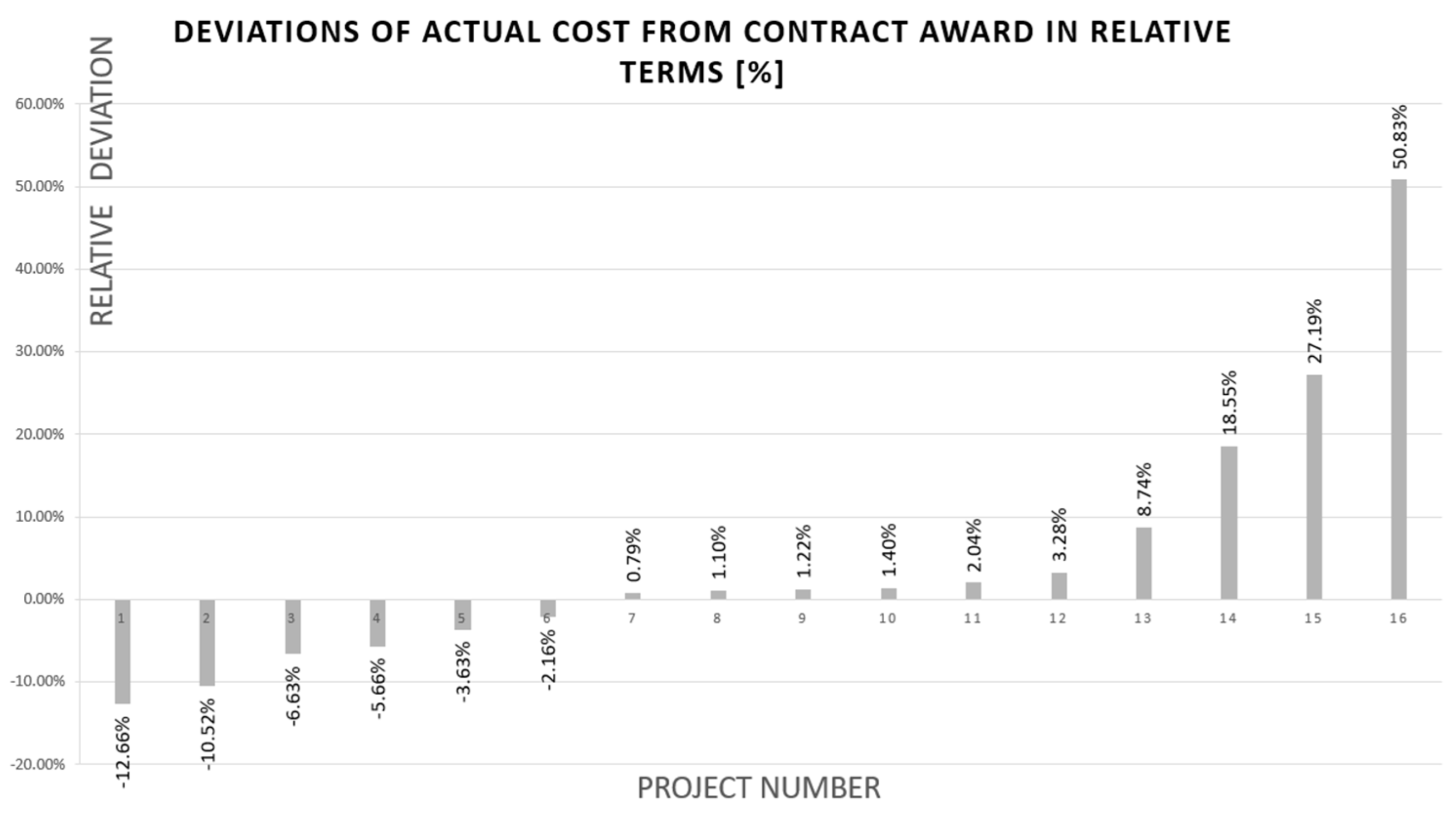
| No. | TUNNELS | Contractually Agreed Costs (TContr) | Final Costs (TFin) | Relative Cost Deviation (TContr − TFin)/TContr |
|---|---|---|---|---|
| 1 | Krpani | 2,984,935.96 €Eur | 3,538,724.73 €Eur | 0.1855 |
| 2 | Sv. Rok | 54,808,956.67 €Eur | 82,669,246.49 €Eur | 0.5083 |
| 3 | Čelinka, Ledenik i Bristovac | 24,020,320.55 €Eur | 26,120,644.90 €Eur | 0.0874 |
| 4 | Dubrava | 9,848,213.18 €Eur | 10,170,756.60 €Eur | 0.0328 |
| 5 | Zaranač i Bisko | 16,187,747.11 €Eur | 16,315,776.96 €Eur | 0.0079 |
| 6 | Sv. Ilija | 27,049,266.41 €Eur | 34,402,808.52 €Eur | 0.2719 |
| 7 | Umac | 5,257,408.48 €Eur | 5,321,491.98 €Eur | 0.0122 |
| 8 | Šubir | 14,685,832.95 €Eur | 14,986,058.55 €Eur | 0.0204 |
| 9 | Mali Prolog | 12,976,806.73 €Eur | 13,158,346.82 €Eur | 0.014 |
| 10 | Kobiljača | 11,678,082.63 €Eur | 11,016,875.75 €Eur | −0.0566 |
| 11 | Puljani | 4,638,079.08 €Eur | 4,537,868.23 €Eur | −0.0216 |
| 12 | Crna Brda | 5,844,625.04 €Eur | 5,229,730.89 €Eur | −0.1052 |
| 13 | Stražina | 8,957,034.30 €Eur | 9,055,351.28 €Eur | 0.011 |
| 14 | Zmijarević | 8,984,025.60 €Eur | 8,388,274.57 €Eur | −0.0663 |
| 15 | Petrovac | 5,805,759.34 €Eur | 5,594,887.11 €Eur | −0.0363 |
| 16 | Međak | 6,836,106.44 €Eur | 5,970,779.93 €Eur | −0.1266 |
References
- Flyvbjerg, B.; Holm, M.S.; Buhl, S. Underestimating Costs in Public Works Projects: Error or Lie? J. Am. Plan. Assoc. 2002, 68, 279–295. [Google Scholar] [CrossRef]
- Love, P.E.; Sing, M.C.; Ika, L.A.; Newton, S. The cost performance of transportation projects: The fallacy of the Planning Fallacy account. Transp. Res. Part A Policy Pract. 2019, 122, 1–20. [Google Scholar] [CrossRef]
- Odeck, J. Do reforms reduce the magnitudes of cost overruns in road projects? Statistical evidence from Norway. Transp. Res. Part A Policy Pract. 2014, 65, 68–79. [Google Scholar] [CrossRef]
- Terrill, M.; Emslie, O.; Moran, G. The Rise of Megaprojects; Geattan Institute: Carlton, Australia, 2020. [Google Scholar]
- Siemiatycki, M. Academics and Auditors Comparing Perspectives on Transportation Project Cost Overruns. J. Plan. Educ. Res. 2009, 29, 142–156. [Google Scholar] [CrossRef]
- Love, P.E.; Ahiaga-Dagbui, D.D. Debunking fake news in a post-truth era: The plausible untruths of cost underestimation in transport infrastructural projects. Transp. Res. Part A Policy Pract. 2018, 113, 357–368. [Google Scholar] [CrossRef]
- Adam, A.; Josephson, P.-E.B.; Lindahl, G. Aggregation of factors causing cost overruns and time delays in large public construction projects: Trends and implications. Eng. Constr. Archit. Manag. 2017, 24, 393–406. [Google Scholar] [CrossRef]
- Durdyev, S. Review of construction journals on causes of project cost overruns. Eng. Constr. Archit. Manag. Emerald Insight. 2020. Available online: https://www.emerald.com/insight/0969-9988.htm (accessed on 5 May 2022). [CrossRef]
- Herrera, R.F.; Sánchez, O.; Castañeda, K.; Porras, H. Cost Overrun Causative Factors in Road Infrastructural projects: A Frequency and Importance Analysis. Appl. Sci. 2020, 10, 5506. [Google Scholar] [CrossRef]
- Tirataci, H.; Yaman, H. Estimation of ideal construction duration in tender preparation stage for housing projects. Organ. Technol. Manag. Constr. Int. J. 2023, 15, 192–212. [Google Scholar] [CrossRef]
- Ershadi, M.; Moghaddam, M.R.; Ezabadi, M.E.R. A competency framework for strategic planning in multi-business holding organisations. Organ. Technol. Manag. Constr. Int. J. 2023, 15, 79–89. [Google Scholar] [CrossRef]
- Catalão, F.P.; Cruz, C.O.; Sarmento, J.M. Public management and cost overruns in public projects. Int. Public 2020, 25, 677–703. [Google Scholar] [CrossRef]
- Sarmento, J.M.; Renneboog, L. Cost Overruns in Public Sector Investment Projects. Public Work. Manag. Policy 2016, 22, 140–164. [Google Scholar] [CrossRef]
- Cantarelli, C.C.; Flybjerg, B.; Molin, E.J.; van Wee, B. Cost Overruns in Large-Scale Transportation Infrastructural projects: Explanations and Their Theoretical Embeddedness. Eur. J. Transp. Infrastruct. Res. 2010, 10, 5–10. [Google Scholar]
- Erol, H.; Dikmen, I.; Atasoy, G.; Birgonul, M.T. Exploring the Relationship between Complexity and Risk in Megaconstruction Projects. J. Constr. Eng. 2020, 146, 04020138. [Google Scholar] [CrossRef]
- Son, J.W.; Rojas, E.M. Impact of Optimism Bias Regarding Organizational Dynamics on Project Planning and Control. J. Constr. Eng. Manag. 2011, 137, 147–157. [Google Scholar] [CrossRef]
- Aljohani, A.; Ahiaga-Dagbui, D.; Moore, D. Construction Projects Cost Overrun: What Does the Literature Tell Us? Int. J. Innov. Manag. Technol. 2017, 8, 137–143. [Google Scholar] [CrossRef]
- Flyvbjerg, B. Survival of the unfittest: Why the worst infrastructure gets built—And what we can do about it. Oxf. Rev. Econ. Policy 2009, 25, 344–367. [Google Scholar] [CrossRef]
- Chen, Y.; Ahiaga-Dagbui, D.D.; Thaheem, M.J.; Shrestha, A. Toward a Deeper Understanding of Optimism Bias and Transport Project Cost Overrun. Proj. Manag. J. 2023, 54, 561–578. [Google Scholar] [CrossRef]
- Osland, O.; Strand, A. The Politics and Institutions of Project Approval—A Critical-Constructive Comment on the Theory of Strategic Misrepresentation. Eur. J. Transp. Infrastruct. Res. 2010, 10, 77–88. [Google Scholar] [CrossRef]
- Flyvbjerg, B. Top ten behavioral biases in project management:An overview. Proj. Manag. J. 2021, 52, 531–546. [Google Scholar] [CrossRef]
- Eliasson, J.; Fosgerau, M. Cost overruns and demand shortfalls-deception or selection? Transp. Res. Part B Methodol. 2013, 57, 105–113. [Google Scholar] [CrossRef]
- Flyvbjerg, B.; Ansar, A.; Budzier, A.; Buhl, S.; Cantarelli, C.; Garbuio, M.; Glenting, C.; Holm, M.S.; Lovallo, D.; Lunn, D.; et al. Five things you should know about cost overrun. Transp. Res. Part A Policy Pract. 2018, 118, 174–190. [Google Scholar] [CrossRef]
- Lovrinčević, M.; Vukomanović, M. Reasons for Cost Overruns in THE Construction of Highways in Croatia. OTMC J. 2022. [Google Scholar]
- Flyvbjerg, B. Quality control and due diligence in project management: Getting decisions right by taking the outside view. Int. J. Proj. Manag. 2013, 31, 760–774. [Google Scholar] [CrossRef]
- Love, P.E.D.; Sing, C.-P.; Carey, B.; Kim, J.T. Estimating Construction Contingency: Accommodating the Potential for Cost Overruns in Road Construction Projects. J. Infrastruct. Syst. 2014, 21, 04014035. [Google Scholar] [CrossRef]
- Cantarelli, C.C.; Molin, E.J.; van Wee, B.; Flybjerg, B. Characteristics of cost overruns for Dutch transport infrastructural projects and the importance of the decision to build and project phases. Transport Policy 2012, 22, 49–56. [Google Scholar] [CrossRef]
- Love, P.E.D.; Wang, X.; Sing, C.-P.; Tiong, R.L.K. Determining the Probability of Project Cost Overruns. J. Constr. Eng. Manag. 2013, 139, 321–330. [Google Scholar] [CrossRef]
- Flyvbjerg, B. Curbing Optimism Bias and Strategic Misrepresentation in Planning: Reference Class Forecasting in Practice. Eur. Plan. Stud. 2008, 16, 3–21. [Google Scholar] [CrossRef]
- Kumar, V.; Pandey, A.; Singh, R. Project success and critical success factors ofconstruction projects: Project practitioners’perspectives. Organ. Technol. Manag. Constr. 2023, 15, 1–22. [Google Scholar]
- Andersen, B.; Samset, K.; Morten, W. Low estimates—High stakes: Underestimation of costs at the front-end of projects. Int. J. Manag. Proj. Bus. 2016, 9, 171–193. [Google Scholar] [CrossRef]
- Love, P.E.; Sing, C.-P.; Wang, X.; Irani, Z.; Thwala, D.W. Overruns in transportation infrastructural projects. Struct. Infrastruct. Eng. Maint. Manag. Life-Cycle 2014, 10, 141–159. [Google Scholar] [CrossRef]
- Odeck, J. Cost overruns in road construction—What are their sizes and determinants. Transp. Policy 2004, 11, 43–53. [Google Scholar] [CrossRef]


| Adam et al. [7] | Durdyev [8] | Herrera et al. [9] |
|---|---|---|
| Communication Financial Management Material Organizational Projects Psychological Weather | Design problems and incomplete design Inaccurate estimation Poor planning Weather Poor communication Stakeholders’ skill, experience, and competence Financial problems/poor financial management Price fluctuations Contract management issues Ground/soil conditions | Failures in design Price variations of material Inadequate project planning Project scope change Design changes Unrealistic contract duration Inadequate bidding method Poor site management and supervision Political situation Legal issues |
| Sample | Shapiro–Wilk Test p-Value | Kolmogorov–Smirnov Test p-Value |
|---|---|---|
| “Road Sections” | 0.07284 | 0.6008 |
| “Viaducts” | 0.07799 | 0.1145 |
| “Tunnels” | 0.6638 | 0.5823 |
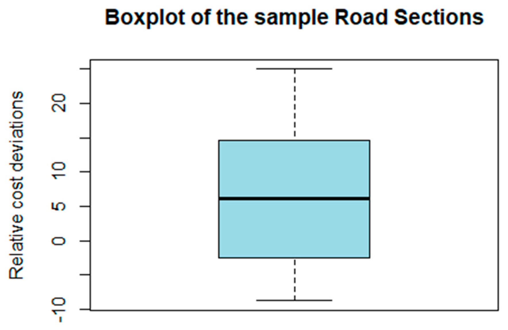
| Min. | Mean | Max | σ | Lower | Upper | Skew |
|---|---|---|---|---|---|---|
| −12.134 | 8.110 | 28.354 | 11.70502 | 3.694841 | 12.52516 | 0.340 |
| Min. | Mean | Max. | σ | Lower | Upper | Skew |
|---|---|---|---|---|---|---|
| −16.73 | −5.23 | 6.27 | 6.69552 | −9.143662 | −1.156338 | 0.498 |
| Min. | 1st Qu. | Median | Mean | 3rd Qu | Max. |
| −12.134 | −2.134 | 7.866 | 7.866 | 17.866 | 27.866 |
| Min. | 1st Qu. | Median | Mean | 3rd Qu | Max. |
| −16.73 | −10.98 | −5.23 | −5.23 | 0.52 | 6.27 |
Disclaimer/Publisher’s Note: The statements, opinions and data contained in all publications are solely those of the individual author(s) and contributor(s) and not of MDPI and/or the editor(s). MDPI and/or the editor(s) disclaim responsibility for any injury to people or property resulting from any ideas, methods, instructions or products referred to in the content. |
© 2024 by the authors. Licensee MDPI, Basel, Switzerland. This article is an open access article distributed under the terms and conditions of the Creative Commons Attribution (CC BY) license (https://creativecommons.org/licenses/by/4.0/).
Share and Cite
Lovrinčević, M.; Vukomanović, M.; Perić, R. Influence of Technical Reasons on Cost Overruns of Infrastructural Projects: A Sustainable Development Perspective. Sustainability 2024, 16, 9413. https://doi.org/10.3390/su16219413
Lovrinčević M, Vukomanović M, Perić R. Influence of Technical Reasons on Cost Overruns of Infrastructural Projects: A Sustainable Development Perspective. Sustainability. 2024; 16(21):9413. https://doi.org/10.3390/su16219413
Chicago/Turabian StyleLovrinčević, Marijo, Mladen Vukomanović, and Romano Perić. 2024. "Influence of Technical Reasons on Cost Overruns of Infrastructural Projects: A Sustainable Development Perspective" Sustainability 16, no. 21: 9413. https://doi.org/10.3390/su16219413
APA StyleLovrinčević, M., Vukomanović, M., & Perić, R. (2024). Influence of Technical Reasons on Cost Overruns of Infrastructural Projects: A Sustainable Development Perspective. Sustainability, 16(21), 9413. https://doi.org/10.3390/su16219413