Modeling the Causes of Urban Traffic Crashes: Accounting for Spatiotemporal Instability in Cities

Abstract

Traffic crashes have become one of the key public health issues, triggering significant apprehension among citizens and urban authorities. However, prior studies have often been limited by their inability to fully capture the dynamic and complex nature of spatiotemporal instability in urban traffic crashes, typically focusing on static or purely spatial effects. Addressing this gap, our study employs a novel methodological framework that integrates an Integrated Nested Laplace Approximation (INLA)-based Stochastic Partial Differential Equation (SPDE) model with spatially adaptive graph structures, which enables the effective handling of vast and intricate geospatial data while accounting for spatiotemporal instability. This approach represents a significant advancement over conventional models, which often fail to account for the fluid interplay between time-varying weather conditions, geographical attributes, and crash severity. We applied this methodology to analyze traffic crashes across three major U.S. cities—New York, Los Angeles, and Houston—using comprehensive crash data from 2016 to 2019. Our findings reveal city-specific disparities in the factors influencing severe traffic crashes, which are defined as incidents resulting in at least one person sustaining serious injury or death. Despite some universal trends, such as the risk-enhancing effect of cold weather and pedestrian crossings, we find marked differences across cities in relation to factors like temperature, precipitation, and the presence of certain traffic facilities. Additionally, the adjustment observed in the spatiotemporal standard deviations, with values such as 0.85 for New York and 0.471 for Los Angeles, underscores the varying levels of annual temporal instability across cities, indicating that the fluctuation in crash severity factors over time differs markedly among cities. These results underscore the limitations of traditional modeling approaches, demonstrating the superiority of our spatiotemporal method in capturing the heterogeneity of urban traffic crashes. This work has important policy implications, suggesting a need for tailored, location-specific strategies to improve traffic safety, thereby aiding authorities in better resource allocation and strategic planning.

1. Introduction

Traffic crashes have become one of the greatest public health threats reported by the World Health Organization (WHO) in 2018, which caused 1.35 million people to die yearly [1]. Consequently, the enduring objective and focus of traffic safety authorities lie in mitigating the occurrence of traffic crashes, lessening the degree of injuries incurred, and reducing the resulting economic losses. Within the realm of road safety, the construction of statistical methodologies to discern the pivotal determinants of traffic crashes has perennially remained a focal point of research [2]. Numerous scholars have underscored the pronounced spatial heterogeneity characteristic of traffic crash occurrences, and in most instances, considering the spatial effects of crashes exhibits superiority over conventional models [3]. To quantify the spatial effects of traffic crashes, an array of advanced statistical models have been harnessed in the spatial modeling of traffic crashes, including random parameter logit models [4,5], conditional spatial autoregressive models [6], and geographically weighted regression models [7], etc. Nonetheless, when quantifying the spatiotemporal heterogeneity of traffic crashes in major urban centers, we are confronted with the task of addressing at least three pivotal challenges:

(a) Threshold demarcation for spatial correlation of urban traffic crashes

Traffic crashes are temporal occurrences within an urban landscape, constituting a spatial point process problem [8]. Certain scholars have retained the spatial point process attributes of traffic crash occurrences, concentrating on the impact of influential variables on the severity of crashes. For instance, Boulieri et al. [9] employed a spatiotemporal multivariate Bayesian model, revealing a distinct interrelatedness in the severity of traffic crashes within various UK cities in terms of both spatial structural and unstructured effects. Liu [10] devised a multivariate spatiotemporal Bayesian model capable of precisely capturing long-term regional trends in traffic collision frequency alterations. Nevertheless, these models are predominantly oriented towards numerical analyses of the effect impacts on the variables of interest. Unraveling the spatial distribution patterns of urban traffic crashes and the spatial correlation between individual crashes remain critical issues to be addressed.

(b) The challenge for adaptive regional division based on urban traffic crash distribution

Some researchers also amalgamate crash data on specific spatial scales and correlate it with various urban characteristics, consequently modeling the impact of feature variables on the frequency of traffic crashes in that area. Existing spatial region partitions usually fall into two categories: areal partitioning including census tract [11], or traffic analysis zone (TAZ) [12], or grid-based partitioning such as regular squares, hexagons [13], etc. For example, the handling of the TAZ has been proven to explain the similarity between different regions, yet it cannot fully capture the extreme spatiotemporal heterogeneity presented by collisions [14]. Grid-based partitioning has also been applied to investigate the impact of road network structural features, and built environment features on the crash frequency within the grid [15,16]. Bao [17] partitioned New York City using grids of different scales and constructed a predictive model based on deep learning. The results showed that the determination of the scale of spatial region partitioning has a significant impact on the predictive results. However, few studies have been devoted to consider the dynamic graph structure of urban traffic crashes simultaneously and compare the spatial heterogeneity of different cities.

(c) The necessity to quantify the influence of time-varying/geographic characteristics on severe traffic crashes

The occurrence of traffic crashes in urban areas is definitively influenced by numerous characteristic factors, encompassing real-time weather conditions and static geographical location information.

Table 1. Summary of research on the impact of weather conditions on traffic safety.

(Author, Year)	Study Area	Weather-Related Variables	Dependent Variables	Model
Abdel-Aty et al., 2011 [19]	Florida	Fog; smoke	Crash severity level	Multilevel ordered logistic model.
Hassan & Abdel-Aty, 2013 [20]	Florida	Visibility; rain; fog	Crash vs. non-crash	Random Forests and matched case-control logistic regression models
Ahmed et al., 2014 [21]	Florida	Fog; non-fog	The number of crashes	Bayesian logistic regression model
Wu et al., 2018 [22]	Florida	Fog	Crash risk increase indicator	Logistic regression model
Zhan et al., 2020 [23]	Shenzhen	Temperature; precipitation	Road traffic casualty	Time-stratified case-crossover analysis; conditional quasi-Poisson regression
Ma et al., 2021 [24]	UK	Rain; wind; fog or mist; snow	Severity of traffic crash	The SSAE-based deep learning model
Madushani et al., 2023 [25]	South Australia	Clear; cloud; fog; rain	Crash severity level	Explainable machine learning

meticulously enumerates some representative literature in this field in recent years. Some studies have revealed that higher wind speeds, lower temperatures and humidity levels further enhance traffic crash injury rates, fatality rates, and severity. However, the relationship between rainfall and crash frequency appears to present a paradoxical phenomenon [18]. The aforementioned research underscores the real-time impact of time-varying covariates yet overlooks the interplay among many factors and the relationship between traffic crashes and spatial dependence.

At present, point of interest (POI) data have evolved into a widely employed novel type of geospatial data, which can collect spatial characteristics and capture highly correlated spatiotemporal data [15]. Leveraging POI data, we can identify the land use type of specific units and aptly describe the level of land use combinations within urban local regions, thereby capturing land use characteristics with higher precision. Pertinent research has unveiled the impact of land use characteristics on the spatial distribution of traffic crashes. Despite the fact that numerous studies have established the link between POI features and crashes, scant research has considered the spatial heterogeneity of this relationship.

In response to the aforementioned issues, we design a spatiotemporal random field model with a stochastic partial differential equation (SPDE) to capture the temporal and spatial heterogeneity of urban traffic crashes. This then sheds light on the effects of real-time weather factors and POI attributes on the occurrence of traffic crashes. We undertake an in-depth composite analysis using traffic crash datasets from three major U.S. cities, New York City, Los Angeles, and Houston, spanning the years 2016 to 2019. New York, Los Angeles, and Houston—three major U.S. cities located in different regions with distinct climatic conditions and urban environments—would provide an ideal setting to compare spatiotemporal patterns of traffic crash severity, offering insights into how diverse factors influence urban road safety across the country. The primary contributions of this study include, but are not confined to, the following:

  (i)

Based on the point process spatial distribution of traffic crashes, we delve into the generic patterns of spatial clustering and correlation among urban traffic crashes.

 (ii)

Using appropriate spatial scales, we aggregate areas exhibiting similar local characteristics of urban traffic crashes, thereby generating an adaptive graph structure for urban traffic crashes.

(iii)

Predicated upon the a priori spatial graph structure of urban traffic, we construct the spatiotemporal random field model with SPDE to eliminate the impact of spatial heterogeneity on model results, thereby unveiling the influence of time-varying characteristics and geographic attributes on the occurrence of severe traffic crashes.

2. Data

This study harnesses the “US-Accidents” large-scale public accident dataset [26], which encompasses approximately 2.8 million crash records occurring across 49 states in the United States from February 2016 to December 2019. The “US-Accidents” dataset proffers an expansive range of data attributes; for each incident, in addition to the severity and category of the crash, it records environmental attributes and other vehicle-related features, such as weather conditions, associated point of interest data, location information, date and start/end time data, the distance affected by the crash, and the severity of delay.

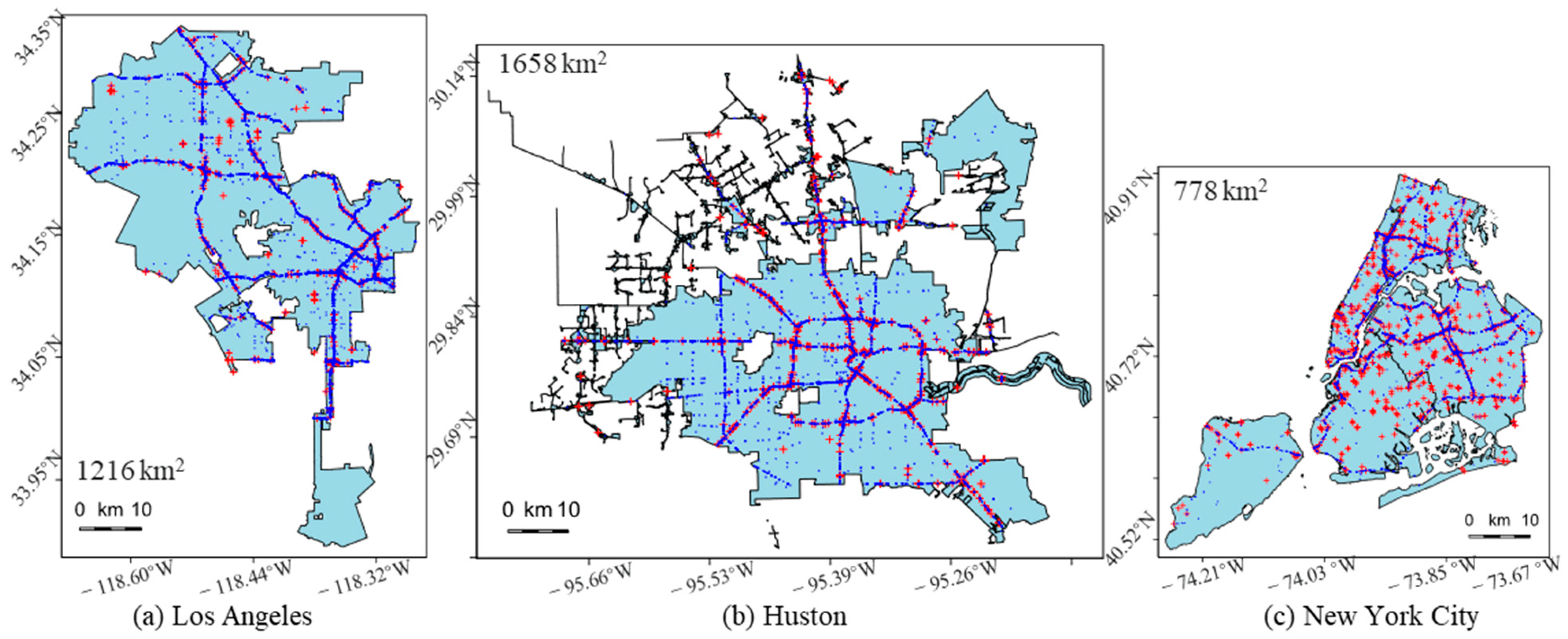
The individual points in spatial road crash analysis each bear a grave significance. Crashes can be categorized into three severity levels: major, minor, and ordinary. The focus of this study is injury severity, especially the impact of major crashes. We represent a major crash occurrence as dummy variable 1, while other severity levels are grouped and represented as dummy variable 0. Spatial distribution maps of traffic crashes in the three cities between 2016 and 2019, based on actual data and scaled identically, are shown in Figure 1. This allows for an intuitive comparison and analysis of crash numbers and distribution characteristics across different cities, uncovering similarities and differences in crash occurrences.

Within traffic crash studies, factors such as temperature, wind speed, precipitation, and visibility are commonly evaluated [27]. Following the classification method for continuous weather variables [28], we have further broken down the weather data as shown in

Table 2. Descriptive statistics of the selected variable.

Variables	New York City		Los Angeles		Houston
	Mean (Std)	[Min, Max]	Mean (Std)	[Min, Max]	Mean (Std)	[Min, Max]
Severity	0.0802	[0, 1]	0.018 (0.132)	[0, 1]	0.054 (0.227)	[0, 1]
Continuous variables
Temperature (°C)	15.1 (9.82)	[−15.6, 36.1]	20.5 (5.86)	[3.28, 39.4]	22.9 (7.45)	[−6.72, 38.0]
Wind speed (m/s)	4.56 (2.39)	[0, 18.5]	2.56 (1.96)	[0, 16.5]	4.03 (1.91)	[0, 12.3]
Time-related attributes
Temperature (°C)
Cold (<0 °C)	0.071(0.257)	[0, 1]	0 (0)	[0, 1]	0.005 (0.069)	[0, 1]
Normal (0–20 °C)	0.566 (0.496)	[0, 1]	0.518 (0.500)	[0, 1]	0.317 (0.465)	[0, 1]
Hot (20–30 °C)	0.326 (0.469)	[0, 1]	0.417 (0.493)	[0, 1]	0.523 (0.500)	[0, 1]
Torrid (>30 °C)	0.037 (0.188)	[0, 1]	0.065 (0.247)	[0, 1]	0.155 (0.362)	[0, 1]
Weather condition
Cloud	0.030 (0.171)	[0, 1]	0.060 (0.238)	[0, 1]	0.019 (0.137)	[0, 1]
Rain	0.074 (0.261)	[0, 1]	0.047 (0.213)	[0, 1]	0.035 (0.185)	[0, 1]
Snow	0.008 (0.091)	[0, 1]	0 (0)	[0, 1]	0 (0)	[0, 1]
Fog	0.009 (0.098)	[0, 1]	0.036 (0.187)	[0, 1]	0.015 (0.119)	[0, 1]
Weekend	0.084 (0.272)	[0, 1]	0.130 (0.336)	[0, 1]	0.083 (0.276)	[0, 1]
Morning peak (6–10)	0.242 (0.428)	[0, 1]	0.170 (0.376)	[0, 1]	0.264 (0.441)	[0, 1]
Morning (10–12)	0.137 (0.344)	[0, 1]	0.137 (0.343)	[0, 1]	0.127 (0.334)	[0, 1]
Launch (12–14)	0.099 (0.300)	[0, 1]	0.144 (0.351)	[0, 1]	0.113 (0.317)	[0, 1]
Afternoon (14–18)	0.204 (0.403)	[0, 1]	0.275 (0.446)	[0, 1]	0.250 (0.433)	[0, 1]
Evening peak (18–21)	0.180 (0.384)	[0, 1]	0.151 (0.358)	[0, 1]	0.130 (0.336)	[0, 1]
Geographical attributes
Amenity	0.039 (0.177)	[0, 1]	0.008 (0.087)	[0, 1]	0.001 (0.031)	[0, 1]
Crossing	0.081 (0.261)	[0, 1]	0.030 (0.170)	[0, 1]	0.029 (0.167)	[0, 1]
Junction	0.265 (0.441)	[0, 1]	0.236 (0.425)	[0, 1]	0.258 (0.438)	[0, 1]
Station	0.041 (0.199)	[0, 1]	0.026 (0.159)	[0, 1]	0.001 (0.036)	[0, 1]
Railway	0.017 (0.130)	[0, 1]	0.010 (0.099)	[0, 1]	0.004 (0.067)	[0, 1]
Stop	0.043 (0.203)	[0, 1]	0.012 (0.109)	[0, 1]	0.008 (0.089)	[0, 1]
Traffic signal	0.128 (0.334)	[0, 1]	0.080 (0.272)	[0, 1]	0.100 (0.300)	[0, 1]

. Firstly, temperature is divided into four categories: cold (below 0 °C), normal (0 to 20 °C), hot (20 to 30 °C), and torrid (above 30 °C). Secondly, weather conditions are classified into cloudy, rainy, snowy, and foggy, with the descriptive statistics for each in Table 2. Lastly, we have focused on seven types of geographical attributes for this study, listed in Table 2.

3. Methods

Urban traffic crashes present a classic spatiotemporal point process issue, with each crash happening at a specific time and location. This study takes into account the spatiotemporal instability of urban traffic crashes, while also exploring the impact of real-time and geographical attributes on severe traffic crash risk. The dependent variable here is whether a traffic crash is severe, a binary category. Covariates include continuous variables like temperature and wind speed, and discrete real-time weather variables and POI attributes. The study aims to (i) explore the spatial correlation of traffic crashes based on their spatial point pattern; (ii) develop an adaptive urban traffic crash spatial graph structure by defining a suitable spatial scale; and (iii) construct a spatiotemporal random field model that aligns with the data’s prior distribution, thereby revealing the effects of covariates and their spatiotemporal instability.

3.1. Nearest Neighbor Function G

To quantify spatial correlation and determine the optimal spatial scale of urban traffic crashes, our attention is first directed towards the arrangement of crash spatial point processes. Often, valuable information regarding the spatial arrangement of points is conveyed through nearest-neighbor distances [29]. Therefore, we employ the nearest-neighbor function, denoted as G, which is utilized to measure the clustering degree of spatial point patterns and is defined as follows:

$$G\left(h\right)={\displaystyle \frac{2}{n\left(n-1\right)d_X\left(h\right)}}{\sum }_{i=1}^n{\sum }_{j=1,j\ne i}^{n}I\left(\left||x_i-x_j|\right|\le h\right)$$

(1)

where $G\left(h\right)$ represents the value of the nearest-neighbor function at distance $h,n$ is the total number of traffic crash points, $d_X\left(h\right)$ denotes the area of a circle with radius $h,x_i$, and $x_j$ denote the spatial positions of two distinct crash points $i$ and $j$, and $I(\cdot )$ is the indicator function. Past studies have demonstrated the effectiveness of the nearest-neighbor function in identifying spatial patterns and determining characteristic spatial scales in various disciplines. By analyzing the behavior of $G\left(h\right)$ at different distance values $h$, we ascertain the critical spatial scale $h^{\ast }$ corresponding to the peak of $G\left(h\right)$. This optimal scale $h^{\ast }$ delineates the characteristic spatial correlation distance of traffic crashes within the urban environment.

3.2. Spatial Interpolation Based on Gridding

To address the irregular spatial distribution of urban traffic crashes and create an adaptive spatial graph structure, we propose a grid-based spatial interpolation algorithm, a widely recognized technique in spatial analysis [30]. This method is effective in generating continuous surfaces from discrete data points, providing a comprehensive understanding of the spatiotemporal patterns. Specifically, the construction of spatial interpolation based on gridding proceeds as follows:

Step1: Delaunay triangulation: Given a set of crash points $X=x_1,x_2,\dots ,x_n$ in 2D space, Delauny triangulation, denoted as $DT\left(X\right)$, connects the points that the circumcircle of each triangle which contains no other points from the input set. $DT\left(X\right)$ is represented as: $DT\left(X\right)=\left(p_i,p_j,p_k\right)|\forall p_i,p_j,p_k\in X$, and the circumcircle of $\left(p_i,p_j,p_k\right)$ contains no other points from $X$. This ensures that the spatial connections between points are optimally established, capturing the underlying spatial structure of crash occurrences.

Step 2: Voronoi subdivision: Based on the Delaunay triangulation, voronoi polygons are constructed, dividing the study area into irregular regions [31]. Each polygon encompasses a crash point and represents its spatial domain of influence. Mathematically, $V\left(X\right)$ is represented as $V\left(X\right)=V\left(p_1\right),V\left(p_2\right),\dots ,V\left(p_n\right)$, where $V\left(p_i\right)$ is the voronoi polygon associated with the crash point $p_i$. This step is crucial as it helps define the spatial extent of each crash point’s influence, allowing us to understand how crashes are distributed across the study area.

Step 3: Grid cell refinement: Crash density within each Voronoi polygon is assessed to guide the refinement of grid cells. Polygons with higher densities are subdivided into smaller grid cells, enhancing the spatial resolution of crash-dense regions. Conversely, polygons with lower densities retain larger grid cells, optimizing computational efficiency without compromising accuracy.

Step 4: Grid-based spatial interpolation: In the gridding method, the spatial region D is divided into N grid cells $D_i$, where i = 1, 2,..., N. Within each grid cell, the spatial data $y\left(s\right)$ and the model $f\left(s,\theta \right)$ are fitted to obtain the estimation result $\widehat{f}(s,\theta )$ within that grid cell, using an objective function that minimizes discrepancies in data representation.

Specifically, we can view each grid cell as a small spatial region $D_i$ within which the following objective function is minimized to solve for the model parameter ${\mathsf{\theta }}_i$.

$${\mathsf{\Theta }}_i={\mathrm{argmin}}_{\mathsf{\theta }}\{-logp(y_{D_i}\left|\theta \right)+logp\left(\theta \right)\}$$

(2)

where $y_{D_i}$ denotes all spatial data within grid cell $D_i$. Here, $p\left(y_{D_i}|\theta \right)$ denotes the conditional probability density function of the spatial data $y_{D_i}$ within the grid cell $D_i$ given the parameter θ. p(θ) is the a priori probability density function which is used to reflect the a priori knowledge of the model parameters.

In order to obtain the estimation result of the whole spatial region, the estimation results within each grid cell can be connected by the interpolation method. Finally, we can obtain the grid-based spatial interpolation algorithm for analyzing urban traffic crashes as shown in Algorithm 1.

Algorithm 1: Grid-Based Spatial Interpolation Algorithm

Input: Spatial data $y\left(s\right)$, spatial region $D$, the number of grid cells $N$ and grid cell size $h_i$, a priori probability density function $p\left(\theta \right)$. Output: Estimation results $\widehat{f}(s,\theta )$ in the spatial region $D$

1: Initialize all parameters in $f\left(s,\theta \right)$ based on prior knowledge or assumptions. Construct triangles such                that no data points lie inside the circumcircle of any triangle, ensuring optimal connectivity between points                and preserving local proximity relationships.                2: Perform Delaunay triangulation to obtain non-overlapping triangles covering spatial region $D$. Divide                region $D$ into polygons where each polygon represents the area of influence around a given crash point $p_i$.                3: Create a Voronoi diagram based on the Delaunay triangulation, dividing $D$ into polygons with single                data points as centroids.                4: Grid-based spatial interpolation:                    a. Divide $D$ into $N$ grid cells $D_i$, where $i=1,2,\dots ,N$ each with size $h_i$.                    b. Within each grid cell $D_i$, fit spatial data $y\left(s\right)$ using Equation (2) to obtain $\widehat{f}(s,\theta )$ for $s\in D_i$, using                    the selected interpolation method.                    c. Utilize interpolation to combine estimates within grid cells to obtain $\widehat{f}(s,\theta )$ for the entire spatial                    region $D$.

3.3. Spatiotemporal Random Field Model with Stochastic Partial Differential Equation (SPDE)

Upon acquiring the adaptive graph structure predicated on the spatial distribution of urban traffic crashes, our attention is directed towards exploring the impact of independent variables on the occurrence of severe traffic crashes. Given the computational challenges posed by large-scale spatial models, we employed the Stochastic Partial Differential Equations (SPDEs) for the approximation of Gaussian random fields, and implement the Integrated Nested Laplace Approximations (INLA) using R-INLA [30,32].

The basic structure of these models presupposes that the traffic crash response (whether it is a severe crash) at any given moment $t$ and location $s$ is a function of fixed effects, spatial effects (capturing the traffic crash evolution process of invariant spatial patterns over year), and the spatiotemporal latent process. Mathematically, the traffic crash prediction for a specific year $t$ at location $s$ can be expressed as follows:

$$\begin{array}{c}\mathbb{E}[y_{s,t}]={\mu }_{s,t}\hfill \\ {\mu }_{s,t}=f^{-1}(X_{s,t}^{main}\beta +O_{s,t}+{\alpha }_g+{\omega }_s+{ϵ}_{s,t})\hfill \end{array}$$

(3)

In our exploration of traffic crashes, we take into account the connected spatial predictions between locations $1:S$ and time $t$, denoted as $u_{s,t}$. In this case, $f^{-1}\left(\cdot \right)$ designates the inverse link function, ${\mathbf{X}}^{main}$ stands for the design matrix of the fixed effects, and $O_{s,t}$ represents an offset: a covariate (typically log-transformed) with a coefficient constrained to one. $\beta$ embodies the estimated parameter vector, ${\mathsf{\omega }}_s$ symbolizes the estimated latent spatial effects, and ${\mathsf{ϵ}}_{s,t}$ signifies the latent spatiotemporal effects for each year.

Both the latent spatial effect ${\mathsf{\omega }}_s$ and the spatiotemporal effect ${\mathsf{ϵ}}_{s,t}$ can be modelled as Gaussian random fields, where ${\mathsf{\omega }}_s$ delineates a spatial intercept that remains invariant with time, and ${\mathsf{ϵ}}_{s,t}$ exemplifies a spatial offset that varies over time. We model the spatial term using $\omega ~MVN(0,{\sum }_{ϵ})$, where the covariance matrix ${\sum }_{ϵ}$ is modeled utilizing the Matérn covariance function. The equation reads as follows:

$$Cov({\omega }_{s_i},{\omega }_{s_j})={\displaystyle \frac{{\sigma }^2}{2^{v-1}{\rm T}\left(v\right)}}(k||x_i-x_j||{)}^v{K}_v(k||x_i-x_j||)$$

(4)

where $K_v(\cdot )$ signifies the modified Bessel function of the second kind, and $v>0$ and $k>0$, respectively, denote the smoothness and scaling parameters. This function is dependent on two hyperparameters: $\sigma$, which modulates the magnitude of the variability, and ${\rm T}\left(v\right)$, which shapes the function.

In terms of modeling the spatiotemporal process, we are presented with multiple alternatives, termed as IID (Independent Identically Distributed) spatiotemporal random fields, which assumes independent spatial variations at each time step for capturing rapid changes in crash patterns:

$$\begin{array}{c}{\mu }_{s,t}=f^{-1}(\dots +{ϵ}_{s,t}+\dots )\hfill \\ {ϵ}_t~MVN(0,{\sum }_{ϵ})\hfill \end{array}$$

(5)

where ${ϵ}_{s,t}$ signifies random field deviations at point $s$ and time $t$, with the assumption that the random fields remain independent across time steps. These spatiotemporal random fields are parameterized internally with a sparse precision matrix:

$${ϵ}_t~MVN(0,{\sigma }_{ϵ}^2{\mathit{Q}}^{-1})$$

(6)

Moreover, we could also model the spatiotemporal process as a first-order auto regressive AR(1) process. This process enriches the spatiotemporal random fields by appending a parameter $\rho$ that defines how crash patterns persist or evolve over successive time steps, which can be defined as follows:

$${\mu }_{s,t}=f^{-1}\left(\dots +{\delta }_{s,t}\dots \right)$$

$${\delta }_{t=1}~MVN(0,{\sum }_{ϵ})$$

(7)

$${\delta }_{t>1}=\rho {\delta }_{t-1}+\sqrt{1-{\rho }^2}{ϵ}_t,{ϵ}_t~MNN(0,{\sum }_{ϵ})$$

where $\rho$ represents the correlation between subsequent spatiotemporal random fields. The $\rho {\delta }_{t-1}+\sqrt{1-{\rho }^2}$ term scales the spatiotemporal variance by the correlation such that it showcases the steady-state marginal variance. The correlation $\rho$ permits mean-reverting spatiotemporal fields and is bound by $-1\le \rho \le 1$.

3.4. Model Goodness-of-Fit Measures

In the methodology of model evaluation, two pivotal statistical tools, the Akaike Information Criterion (AIC) and the Bayesian Information Criterion (BIC) [33], are employed to strike a balance between the goodness-of-fit and the complexity of the model. The definition of AIC and BIC can be formulated as follows:

$$\begin{gathered} AIC=2k-2ln\left(L\right) \\ BIC=ln\left(n\right)\times k-2ln\left(L\right) \end{gathered}$$

(8)

where $k$ denotes the number of model parameters, $L$ represents the maximum value of the likelihood function of the model, and $n$ is the sample size. In the present study, we utilize both AIC and BIC to robustly evaluate and compare the performance and reliability of our constructed models.

4. Results and Discussion

This paper uses data from New York, Los Angeles, and Houston, USA, from 2016 to 2019 to validate the proposed methodology. Initially, we examine the spatial clustering and correlation of the urban traffic crash distribution, performing comparative analyses across the three cities. We then construct a spatially adaptive graph structure of traffic crash distribution characteristics for each city based on this spatial resolution. Finally, we uncover the influence of real-time weather variables and static geographic location features on severe urban traffic crashes’ occurrences, after adjusting for urban spatial heterogeneity.

4.1. Capturing the Spatial Distribution Patterns of Urban Traffic Crashes

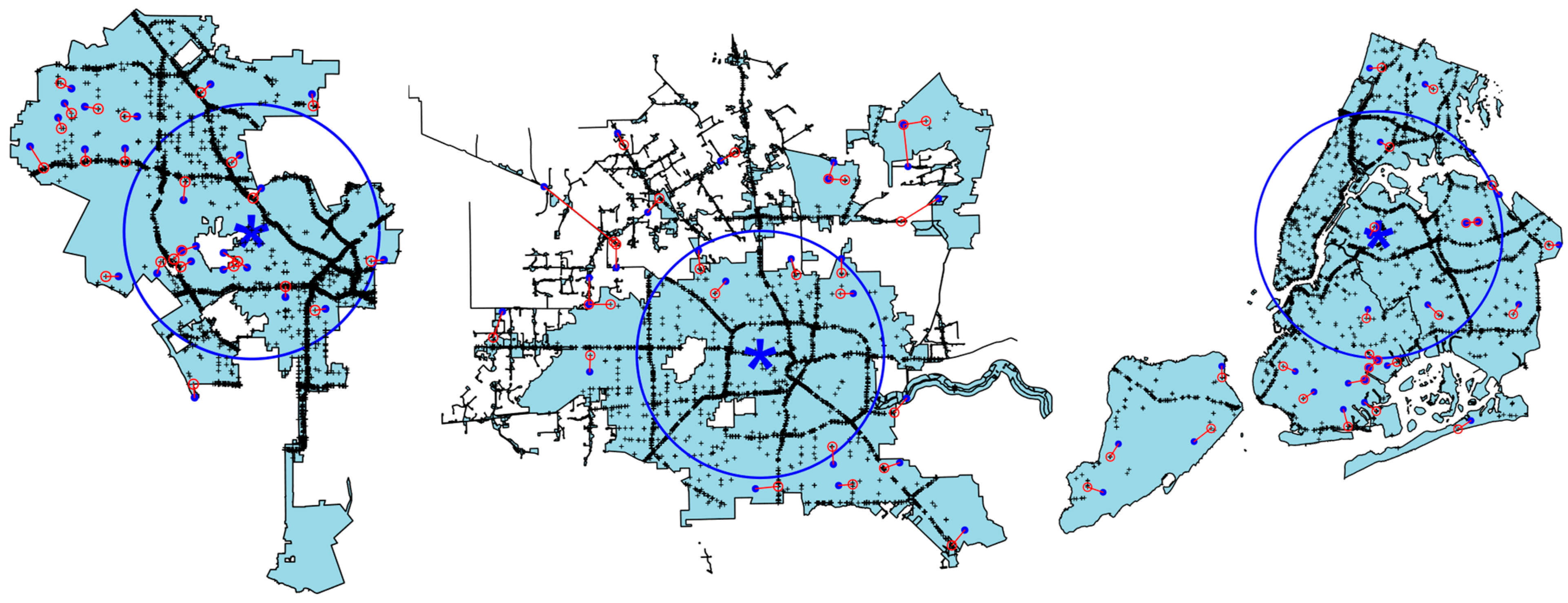
We used a simple mean and variance method to determine the center of gravity of urban traffic crashes and the major areas they covered, as indicated by the blue star and blue circle in Figure 2. From a demographic, economic, and social structure perspective, these areas are typically the core regions of the city. Similarly, research by Moradi et al. [34] also indicated that variables such as population are often directly proportional to the frequency of traffic crashes.

Moreover, we constructed a distance function to calculate the distance between crash points, yielding a distance matrix between crash points. From this, we extracted the distance to the nearest crash point for each crash location and calculated the average shortest distances to be 106.16 m, 70.93 m, and 175.03 m for New York, Los Angeles, and Houston, respectively. This is logical, as Houston, the largest city in terms of area, has the greatest shortest distance between crashes. On the other hand, the ranking of the smallest crash distance is consistent with the city’s crash density ranking (HS(1.81 × 10⁻⁶) < NY(4.37 × 10⁻⁶) < LA(4.72 × 10⁻⁶)). Furthermore, where do isolated crashes typically occur? We plotted the top 25 pairs of crashes with the longest distances apart. As shown in Figure 2, red lines connect the 25 pairs of crashes with the longest distances in each city. Clearly, most isolated crashes occur in non-core areas of the city, while virtually no isolated crashes occur within the core area, i.e., within the blue circle.

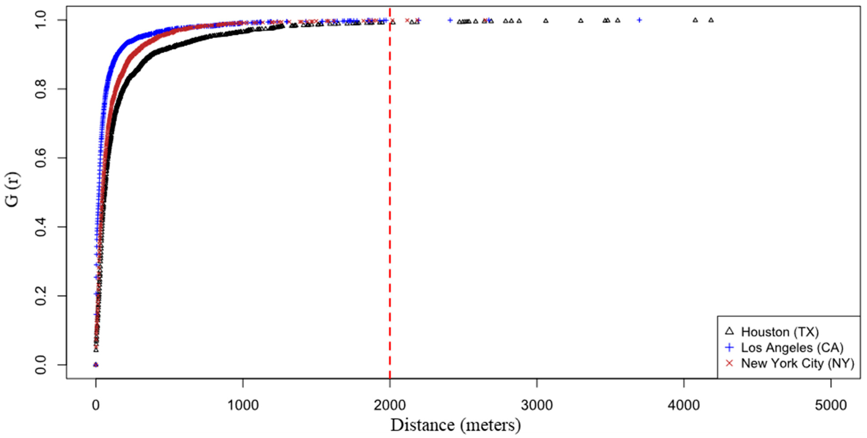
Furthermore, by analyzing the shape of the G-function, we can judge whether there is a phenomenon of spatial clustering or dispersion in the point pattern. Figure 3 shows the estimated nearest-neighbor distance distribution function G(r) for spatial point patterns of the three cities.

Reading from Figure 3, we can find that although these three cities’ structures are different, their patterns are very similar. At about r = 100 m, a value of G(r) = 0.5 is reached, so the median of the nearest neighbor distance distribution of the three cities is approximately 100 m. In addition, the steepness of the line is LA > NY > HS, indicating that the point pattern of traffic crashes in Los Angeles is the most concentrated in space, while the point pattern in Houston is the most dispersed compared to the other two cities. This is also consistent with the order of average crash density obtained for the three cities previously, further proving the existence of strong spatial correlation in crash occurrence. For the distance of 2000 m, we marked it in red on Figure 3, which covers 99% of the neighbors. Many scholars, when studying spatial areas, often set the spatial resolution at 2 km based on experience and computational efficiency [35]. This paper also proves the reasonableness of such a setting from the perspective of the underlying mechanism.

4.2. Adaptive Graph Structure of Urban Traffic Crashes

Considering this, it is imperative to consider the spatial correlation of crashes when studying their occurrence point patterns. Many researchers divide cities into several grids (usually regular quadrilaterals or hexagons) for further study, thus considering the spatial feature. However, different cities have heterogeneous geographical structures and crash distributions.

To address this challenge, we propose an algorithm that adaptively constructs a spatial graph structure based on city maps and crash distribution. The SPDE method decomposes the continuous spatial domain into discrete grids and then models the local characteristics of Gaussian random fields on each grid [36]. On each grid, partial differential equations are used to describe the changes and spatial correlations of Gaussian random fields, thereby converting the continuous Gaussian random fields into a discrete form.

Ultimately, we obtained the spatial adaptive graph structure of traffic crashes as shown in Figure 4. In Figure 4, we divide the space into a set of non-overlapping triangles that intersect at most on a common side or corner. In areas with a high density of crashes, the triangular area is smaller, while in areas with sparse crashes, the triangular area is larger. This result effectively achieves a sparse approximation of the random distribution of crashes, and a graph structure more closely matched to the current research area is of significant importance for further exploration of the spatial homogeneity of urban traffic crashes.

4.3. Spatiotemporal Field Model for Traffic Crashes

Building on the traffic crash spatial graph structure from the previous section, we employed a 2 km spatial resolution for our analysis, which was identified through exploratory spatial analysis as the scale that best captured significant crash clustering. This resolution enabled our model to accurately detect localized crash hotspots while preserving the broader crash distribution patterns across different neighborhoods. For the temporal analysis, we addressed annual instability by examining crash data spanning multiple years (2016–2019), allowing us to capture fluctuations in crash severity patterns influenced by factors such as weather conditions, traffic volumes, and infrastructure changes. By incorporating annual temporal variability, our model provided a comprehensive view of how crash severity factors evolved over time, yielding insights into long-term trends and the shifting impact of different influences on crash severity across years.

Finally, we constructed spatial effect models and spatiotemporal effect models for the occurrence patterns of traffic crashes. For reference, the traditional fixed-effect model was also estimated. The fitting results of the final models are shown in

Table 3. Goodness-of-fit measures for the estimated models.

	Los Angeles	New York	Houston
	Model1/Model2/Model3	Model1/Model2/Model3	Model1/Model2/Model3
Goodness-of-fit
No. of observations	20,543	10,268	10,078
No. of parameters	19/21/22	21/23/24	20/22/23
Log-likelihood	−6210.575/−6185.847/−6051.243	−2558.75/−2414.32/−2387.65	−2033.57/−1999.62/−1952.07
AIC	12,459.15/12,413.69/12,146.49	5159.56/4874.71/4823.30	4107.14/4043.24/3950.14
BIC	12,609.89/12,580.30/12,321.02	5311.83/5041.47/4997.40	4251.52/4202.06/4116.18
AUC	0.79/0.80/0.83	0.72/0.77/0.78	0.75/0.76/0.79
Spatiotemporal characteristics
Matérn range	--/2.48/19.3	--/6.27/5.99	--/10.07/17.4
Spatial SD (sigma_O)	--/0.479/0.064	--/1.26/1.20	--/1.00/0.93
Spatiotemporal SD (sigma_E)	--/--/0.471	--/--/0.85	--/--/0.719

. It can be seen that both the spatial effect model and the spatiotemporal effect model significantly outperform the traditional model, with the spatiotemporal effect model performing the best. In Table 3, Model1 refers to the traditional fixed-effect model, Model2 refers to the spatial effect model, and Model3 refers to the spatiotemporal effect model.

In Table 3, the Matérn range reflects the scale or distance of spatial correlation [32]. Los Angeles (19.3) and Houston (17.4) exhibit larger values, indicating a spatial correlation in crash severity over larger distances, while New York (5.99) has a smaller value, indicating correlation decays over a shorter distance. Spatial standard deviation (SD) measures the variability or dispersion of crash severity in space. New York’s highest value (1.20) suggests the greatest spatial variability in crash severity, followed by Houston (0.93), and Los Angeles has the smallest variability with 0.064. Spatiotemporal SD, measuring the variability or dispersion of crash severity in space and time, is highest in New York (0.85), suggesting that time and space factors significantly influence crash severity compared to Los Angeles (0.471) and Houston (0.719).

We also considered time-related weather condition variables and used POI attributes to measure city structure in models for the three cities. Specifically, we constructed traditional fixed effect models, spatial effect models, and spatiotemporal effect models for each city. Due to constraints on the length of the article, the results of the spatiotemporal effect models are only presented in

Table 4. Consolidated estimation results of spatiotemporal effect models for Los Angeles, New York, and Houston.

	Los Angeles		New York		Houston
	Mean (SD)	95% BCI	Mean (SD)	95% BCI	Mean (SD)	95% BCI
Intercept	−2.64 (0.266)	(−3.16, −2.12)	−3.13 (0.458)	(−4.03, −2.23)	−2.87 (0.422)	(−3.69, −2.04)
Real-time characteristics
Temperature (°C)
Cold	-	-	0.865 (0.437)	(0.0089, 1.72)	0.764 (0.572)	(−0.357, 1.89)
Normal	0.284 (0.241)	(−0.188, 0.755)	0.411 (0.371)	(−0.316, 1.14)	−0.307 (0.272)	(−0.84, 0.225)
Hot	0.294 (0.228)	(−0.154, 0.741)	0.41 (0.36)	(−0.296, 1.12)	−0.201 (0.237)	(−0.665, 0.263)
Torrid	0.213 (0.26)	(−0.298, 0.723)	0.012 (0.456)	(−0.882, 0.906)	−0.358 (0.288)	(−0.921, 0.206)
Weather conditions
Cloud	0.111 (0.122)	(−0.129, 0.351)	−0.0532 (0.251)	(−0.544, 0.438)	0.459 (0.249)	(−0.0289, 0.947)
Rain	−0.43 (0.125)	(−0.675, −0.185)	0.362 (0.151)	(0.066, 0.658)	0.277 (0.213)	(−0.14, 0.694)
Snow	-	-	0.378 (0.404)	(−0.415, 1.17)	-	-
Fog	0.244 (0.126)	(−0.00275, 0.491)	−0.161 (0.48)	(−1.1, 0.779)	0.216 (0.334)	(−0.439, 0.871)
Spatial characteristics
Amenity	−0.661 (0.473)	(−1.59, 0.266)	0.958 (0.166)	(0.633, 1.28)	-	-
Crossing	0.0604 (0.193)	(−0.318, 0.439)	0.407 (0.144)	(0.125, 0.689)	0.266 (0.354)	(−0.427, 0.96)
Junction	0.136 (0.0566)	(0.0249, 0.247)	−0.658 (0.119)	(−0.892, −0.424)	0.258 (0.109)	(0.0434, 0.472)
Station	−0.187 (0.226)	(−0.63, 0.257)	1.08 (0.166)	(0.758, 1.41)	-	-
Railway	−0.377 (0.321)	(−1, 0.252)	0.368 (0.256)	(−0.133, 0.869)	−1.19 (1.08)	(−3.3, 0.917)
Stop	−0.201 (0.266)	(−0.723, 0.321)	0.574 (0.187)	(0.207, 0.94)	−0.0491 (0.614)	(−1.25, 1.15)
Traffic_Signal	−0.348 (0.125)	(−0.594, −0.103)	0.756 (0.123)	(0.515, 0.998)	−0.231 (0.204)	(−0.631, 0.169)
Smooth terms
Wind speed (km/h)	2.00 (3.73)		−1.90 (0.55)		0.36 (0.31)
Temperature (°)	−1.84(0.53)		1.11(0.63)		−0.09(0.83)

.

4.3.1. Heterogeneity in the Influence of Real-Time Weather Factors

This section examines how real-time weather conditions impact severe crash risks across three cities. Low temperatures (below 0 °C) in New York and Houston increase severe crash risks. As Los Angeles temperatures never drop below zero, no fit parameters apply here. Interestingly, hot weather elevates severe crash risks in New York and Los Angeles but reduces it in Houston. With New York and Los Angeles having cooler climates compared to Houston’s hot and humid conditions, their drivers may be less prepared for high-temperature driving, increasing severe crash risks. Houston residents, familiar with hot conditions, have developed better driving habits under such circumstances, thus reducing crash risks.

In terms of weather conditions, rainy weather boosts severe crash risks in New York and Houston but lessens it in Los Angeles. Annual average rainfall and rainy days in these cities show that New York and Houston have high rainfall while Los Angeles receives less. Thus, less rainy cities like Los Angeles may practice more caution during rainfall, reducing severe crash risks. This indicates unobserved heterogeneity like psychological factors and regional climate characteristics that significantly influence severe crash risks [37].

4.3.2. Heterogeneity in the Influence of Urban Built Environments

To assess how spatial heterogeneity in urban built environments affects traffic crash severity, this section specifically analyzes how various traffic facilities like crossings, junctions, traffic signals, stations, railways, and stops impact crash severity in New York, Los Angeles, and Houston.

The presence of crossings has a positive effect on the occurrence of severe traffic crashes, and among the three cities, the positive effect is strongest in New York. This is mainly because the crossing is often located in high-traffic areas, significantly increasing severe traffic crashes, particularly in New York, a global economic hub with heavy daily pedestrian and vehicle traffic.

In terms of junctions and traffic signals, the impact on crash severity varies among the cities. Junctions decrease crash severity risk in New York but increase it in Los Angeles and Houston. Traffic signals, on the other hand, increase crash severity risk in New York but decrease it in Los Angeles and Houston. With fewer intersections and longer roads, Los Angeles and Houston have higher average driving speeds. Drivers may fail to adequately adjust their speed or behavior at uncontrolled intersections, raising the risk of severe crashes [38]. Traffic characteristics and infrastructure diversity explain varying coefficients for stations, railways, and stops across the cities. In New York, the positive coefficients suggest these transport facilities may increase severe crash risks [39]. In Los Angeles and Houston, the negative coefficients for railways and stops suggest they may mitigate crash severity.

4.3.3. City-Specific Insights

Our study uncovered distinct patterns of crash severity factors across New York, Los Angeles, and Houston, highlighting the importance of tailored, city-specific traffic safety strategies. In New York, cold weather, particularly temperatures below 0 °C, significantly increased the risk of severe crashes, suggesting that icy or snowy conditions create hazardous driving environments. Pedestrian crossings also emerged as a key factor contributing to crash severity, likely due to the city’s high pedestrian traffic and dense urban core, indicating that enhancing road safety measures during winter and improving pedestrian infrastructure could be effective in reducing severe crashes. In Los Angeles, foggy conditions were found to be a significant contributor to severe crash, emphasizing the need for improved visibility measures in such weather. Junctions were associated with an elevated risk of severe crashes, likely influenced by high-speed traffic and less controlled intersections, while traffic signals showed a mitigating effect, indicating their importance in managing crash risks. These findings suggest that traffic safety efforts in Los Angeles should prioritize visibility enhancements during foggy conditions and implement additional safety measures at junctions. In Houston, rainfall emerged as a significant factor in increasing risk of severe crash, suggesting that wet road conditions are a primary risk factor. Unlike Los Angeles, junctions were less strongly associated with severe crashes, but the presence of traffic signals still played a crucial role in reducing crash severity. To improve safety in Houston, interventions should focus on road safety measures during rainy conditions, such as improving road drainage and using anti-skid surfacing, alongside optimizing traffic signal operations. The differences observed among the three cities underscore the need for location-specific traffic safety strategies that address unique weather conditions, traffic patterns, and infrastructure.

5. Conclusions

In our research, we employed a spatiotemporal random field model with a stochastic partial differential equation (SPDE) to delve into the spatiotemporal heterogeneity of traffic crashes and analyze the differing factors influencing crash severity in New York, Los Angeles, and Houston. This approach lets us incorporate geospatial data’s spatial correlation into the statistical model and handling of large-scale geospatial data.

Our key findings include the following: Analysis of traffic crash distribution’s spatial clustering and correlation in various cities supports a 2 km granularity for spatiotemporal analysis which strikes a balance between computational resources and analytical precision. An adaptive graph structure for urban traffic crashes is built using a grid-based spatial interpolation method, to estimate and eliminate spatial autocorrelation in the model. Lastly, an SPDE model was constructed to assess the differing impacts of real-time weather conditions and urban built environment factors on crash severity. Our results showed that cold weather significantly increases the risk of severe traffic crashes in New York and Houston, while hot and rainy weather influences crash severity differently across the cities. The presence of pedestrian crossings was found to consistently raise the likelihood of severe crashes in all three cities, although the influence of other traffic facilities varied by location. Specifically, in New York, cold weather and pedestrian crossings were significant contributors to crash severity, indicating the need for improved safety measures during winter and at pedestrian crossings. In Los Angeles, foggy conditions increased crash severity, and junctions posed a higher risk, highlighting the importance of visibility enhancements and additional safety measures at intersections. In Houston, rainfall significantly elevated crash severity, emphasizing the need for road safety improvements during wet conditions.

These findings can guide regulatory authorities to improve traffic safety. Authorities should enhance road condition monitoring and snow clearance, provide weather and road condition updates, and improve junction visibility for common patterns like cold weather effects and crossings. Our study suggests several policy recommendations to reduce traffic crash severity in urban areas. Authorities should implement weather-responsive road treatments, such as proactive salting, de-icing, and improved drainage in cities affected by cold or rainy conditions, as seen in New York and Houston. Enhancing pedestrian safety with better lighting, clear signage, and raised crosswalks at high-traffic crossings, alongside introducing more controlled intersections like roundabouts in high-risk areas of Los Angeles, can also mitigate severe crashes. Increased traffic enforcement during high-risk hours, through DUI checkpoints and automated speed monitoring, combined with investing in real-time traffic monitoring systems, will enable quicker responses to congestion and incidents. By integrating these measures, cities can effectively address crash severity factors and improve overall road safety. Importantly, these recommendations are not only relevant for large cities but also provide valuable guidance for smaller urban areas, aiding in the improvement of traffic safety across different city sizes and contexts.

While the model effectively captured spatiotemporal patterns, potential inaccuracies in crash reporting and the binary classification may limit the full representation of the severity, and its generalizability to other cities requires further validation. Future research will focus on adopting more nuanced classification approaches, such as ordinal or multinomial models, to capture the full range of crash severity and provide a deeper understanding of traffic safety dynamics. Additionally, we plan to extend the application of our model to international cities with diverse traffic systems, climates, and urban infrastructures, as well as to smaller or suburban regions with distinct traffic patterns. These efforts will enable us to assess the model’s adaptability and robustness in capturing crash severity across different urban environments, ultimately contributing to the development of more targeted and effective interventions to reduce crash risks at all severity levels.