Abstract
This paper addresses the challenges and opportunities associated with integrating grid-forming inverters (GFMs) into modern power systems, particularly in the presence of nonlinear loads. Nonlinear loads introduce significant harmonic distortions in the source voltage and current, leading to reduced power factor, increased losses, and an overall reduction in system performance. To mitigate these adverse effects, active filters are employed. The objective of this study is to investigate a synergistic approach to modeling and control in integrated power systems with GFMs, focusing on enhancing power quality and grid stability by reducing harmonic distortions through the use of voltage-source active filters. This research contributes to sustainability by supporting the reliable and efficient integration of renewable energy sources, thereby reducing dependency on fossil fuels and minimizing greenhouse gas emissions. Additionally, improving power quality and system efficiency helps reduce energy waste, which is crucial for achieving sustainable energy goals. Simulations are conducted on a 1000 kW GFM connected to a grid with a nonlinear variable load, demonstrating the system’s effectiveness in adapting to dynamic conditions, reducing harmonics, and promoting a stable, resilient, and sustainable power grid.
1. Introduction
Modern power systems increasingly integrate distributed electrical power generation sources that often use power electronic converters to connect and interact with the main grid. These converters can possess grid-forming capabilities, allowing them to independently regulate voltage and frequency, ensuring stability even without the main grid. They are termed GFMs. Their control mimics the function of traditional synchronous generators, enhancing grid stability and resilience in the face of increasing renewable energy penetration [1,2,3]. This research is particularly relevant in the context of sustainability, as GFMs are essential for integrating renewable energy sources such as solar and wind into power systems. By enabling decentralized control and enhancing grid stability, GFMs support a transition away from fossil fuel-based power generation, contributing to reduced greenhouse gas emissions and a more sustainable energy future.
Non-linear loads connected to the system are a major contributor to the degradation of power quality in system networks. These loads, such as rectifiers, variable frequency drives, and various power electronic devices, draw current in a non-sinusoidal manner, leading to the generation of harmonic currents. These harmonic currents, which are multiples of the fundamental frequency, interact with the system impedance, causing harmonic voltages that distort the overall voltage waveform across the network. These distortions degrade power quality, increase energy losses, and reduce overall system efficiency, leading to higher energy consumption and a larger carbon footprint. Addressing these issues through power filtering contributes directly to sustainability by improving energy efficiency and reducing the adverse environmental impact of inefficient power systems.
The filters normally used are passive and cannot adapt to changes in source impedance, load parameters, or system configurations. Passive filters are designed to provide fixed compensation for specific reactive power and harmonic conditions. Passive filters can become detuned due to variations in system requirements, diminishing their effectiveness. They may experience series and parallel resonance with line impedance, further degrading their performance and overall power quality [4,5]. Active filters provide a dynamic solution by offering adaptive harmonic compensation that automatically adjusts to changes in the power system. Active filters maintain high efficiency and superior harmonic distortion reduction under nonlinear, variable load conditions. By improving voltage and current waveforms, active filters enhance overall power quality, supporting the reliable operation of distributed energy resources and facilitating the integration of clean energy sources [6,7]. In this way, active filters not only improve power quality but also reduce the need for additional conventional generation to compensate for power losses, thus contributing to sustainable energy management.
Active filters are advanced power electronic devices that dynamically compensate for harmonic distortions by adjusting their filtering characteristics in real time. They are simply bidirectional converters; in one direction, they operate as rectifiers to charge the filter capacitor, while in the other direction, they function as inverters to generate the required harmonics. Thus, active filters utilize improved voltage source converters to provide the necessary harmonic and reactive power compensation. The specific compensation method depends on whether the active filter is configured as a shunt or series active filter. The shunt active filter (SAF) targets current harmonics, whereas a series active power filter used in series with loads mitigates grid voltage harmonics by generating negative voltage harmonics to cancel load voltage effects and maintain a pure sine shape against transients, sag, and swell events [8]. Focusing on mitigating grid current harmonics, this paper discusses the control of an SAF for harmonic elimination.
SAFs dynamically filter out harmonics from the source current by continuously monitoring the load current, extracting the harmonic content, calculating the required compensating current, and injecting this current into the power system. They detect harmonics by measuring distorted currents from non-linear loads, extracting harmonic components using algorithms like fast Fourier transform, and generating a reference compensating current based on the extracted harmonics. The SAF injects the compensating current into the point of common coupling (PCC) to cancel out harmonics, resulting in a pure sinusoidal waveform [9,10].
Several practical considerations are crucial for the effective performance of an SAF. Firstly, the SAF must be appropriately rated to match the system’s power levels, harmonic content, and reactive power compensation needs; undersizing can lead to inadequate compensation, while oversizing may incur unnecessary costs. The choice of control strategies—such as hysteresis, PI-based, or predictive control—affects the accuracy and responsiveness of harmonic correction, with well-designed algorithms essential for real-time stability. Additionally, it is essential to ensure proper synchronization at the PCC during integration, along with compatibility with protective measures [11,12].
A detailed control architecture is presented in Figure 1, where the GFM operates in tandem with an SAF to ensure stable, high-quality power delivery in the presence of nonlinear loads and grid disturbances. The ability of this combined system to dynamically manage and compensate for power requirements ensures that renewable energy sources can be reliably integrated, reducing reliance on fossil fuel generation and supporting global efforts toward sustainability and energy efficiency. The diagram can be divided into several key components and control loops that work together to maintain stable operation and improve power quality. The inverter is depicted through its equivalent voltage source Einv, which operates with a specific phase angle δinv. This model highlights the inverter’s ability to deliver both active power Pinv and reactive power Qinv to the grid. The grid’s voltage E and frequency ω serve as the reference points that guide the inverter’s operation, ensuring that it functions in sync with the grid’s conditions [13].
The primary control loop, referred to as droop control, plays a critical role in managing the GFM’s operation. This loop adjusts the inverter’s output frequency δref and voltage reference Eref based on the active power P and reactive power Q it generates, following predefined droop characteristics. This approach is essential for stabilizing the grid, as it allows the inverter to operate independently without needing an external synchronization signal. Additionally, voltage and current controllers ensure that the inverter’s output voltage and the current injected into the grid are regulated within safe operational limits, adhering to the references set by the droop control. The phase-locked loop (PLL) further supports this process by synchronizing the inverter’s output with the grid, accurately tracking the grid voltage phase θ, and maintaining the inverter’s operation in phase with the grid.
The SAF is engineered to reduce harmonics and enhance power quality by injecting compensating currents if into the system. The current controller regulates this injected current and ensures that it aligns with the reference current, which is specifically calculated to cancel out the harmonics present in the load current IL. The reference current calculation is derived directly from the load current, determining the necessary compensating current to effectively mitigate harmonics. Also, DC voltage control is important to keep the shunt filter’s DC link voltage at the target reference level (VDC_ref), which is essential for effective harmonic compensation [9,14]. The nonlinear load model represents the grid’s connection to a combined resistive–inductive load, which imposes both active and reactive power demands on the system. The inverter, along with the SAF, must dynamically manage and compensate for these power requirements to maintain grid stability and power quality. The interaction between the GFM and the SAF is depicted in the figure, with red dotted lines representing the flow of control signals and power references between these components. The inverter’s primary responsibility is to maintain the grid’s voltage and frequency, while the active filter focuses on improving power quality by mitigating harmonics and stabilizing the DC link voltage [15,16].
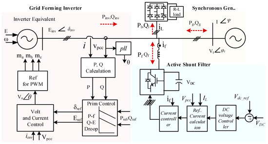

Figure 1.
Integrated power system network [16].
Figure 1.
Integrated power system network [16].
2. Integrated System Control
The inverter is designed to create a stable voltage and frequency reference for the grid, effectively ‘forming’ the grid itself. It can operate independently or in conjunction with other grid components to establish the grid parameters, especially in systems with a high penetration of intermittent renewable energy sources. The control of this inverter is based on the droop characteristics of active and reactive power with voltage and frequency, respectively. Droop control is a decentralized control method that allows inverters to share loads without requiring communication between them by adjusting their output power based on the local frequency and voltage measurements. Figure 2 illustrates the droop control strategy.
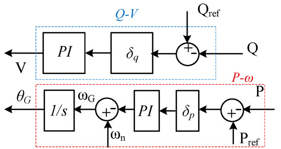
Figure 2.
Droop control of grid-forming inverter [3,16].
The main purpose of the active power droop control loop is to adjust the inverter’s output frequency by regulating the active power output. The control loop uses a droop characteristic, which is a linear relationship between the frequency deviation and the active power output. Similarly, the reactive power droop control loop’s main purpose is to adjust the inverter’s output voltage to regulate the reactive power output. The equation for the droop control can be expressed as:
Here, are the droop coefficients for active and reactive power. From these equations, if the active power demand increases, the inverter will decrease its output frequency to balance the power; and if the reactive power demand increases, the inverter will decrease its output voltage to balance the power. Proportional–integral controllers regulate the voltage and frequency to ensure that the reactive and power output meet the references Qref and Pref, respectively. The outputs of these controllers adjust the reference values for the inverter, ensuring that it responds to load changes and maintains the grid’s stability. Thus, the droop control strategy allows GFMs to autonomously share the load by adjusting their output frequency and voltage based on local measurements, ensuring a stable and balanced power supply in a decentralized manner [17,18].
To model the integrated system, system equations must be developed that account for the power balance between generation and load. The SAF injects compensating currents to mitigate the harmonics in the source current caused by non-linear loads. The filter current depends on the load current’s harmonic component and the PCC voltage (3).
The filter’s objective is to ensure the current drawn from the source remains sinusoidal. Non-linear loads introduce harmonics, affecting the source current and voltage. The non-linear load current Iload can be decomposed into fundamental and harmonic components.
The power balance equation at the PCC can be presented as (5).
The voltage at the PCC is influenced by the GFM inverter (7). This equation expresses the relationship between the voltage at the PCC and the voltage output of the GFM inverter, considering the line’s impedance and the difference between the load current and the filter current. The equation shows that the PCC voltage is influenced by the GFM inverter’s voltage and is subject to a voltage drop across the line impedance, which depends on the net current (i.e., the difference between the load current and the filter current). This illustrates how the GFM inverter can control the voltage at the PCC, with the line impedance playing a crucial role in this interaction.
The frequency at the PCC is influenced by both the SG and the GFM inverter (8). It describes how the frequency at the PCC is influenced by the power contributions from both the synchronous generator (SG) and the GFM inverter.
The frequency at the PCC is determined by the net power balance, with the contributions from the SG and GFM inverters influencing it. The load’s power demand (adjusted for filter compensation) and losses tend to oppose changes in frequency. The system’s moment of inertia Jsys acts as a dampening factor, moderating the impact of power imbalances on frequency changes. This equation highlights the critical role of the GFM inverter and SG in maintaining stable frequency at the PCC, which is essential for overall system stability, especially in scenarios involving varying loads or disturbances [19].
Control of Shunt Active Filter
The SAF control involves detecting and analyzing the harmonic components in the load current and then generating appropriate compensating currents to cancel out the harmonics from the source currents. The control strategy ensures that the currents injected by the SAF are in phase with the harmonics of the load current, thereby achieving effective harmonic suppression. The mathematical foundation of this control algorithm can be expressed through a series of equations that govern the detection, analysis, and compensation processes. The load current comprises fundamental current drawn from the sources and the various harmonics.
Load power can be the product of voltage across the load (almost the same as the source, voltage at PCC) and current through the loads.
For the source current to be sinusoidal at the unity power factor, the source power should be equal to the fundamental power,
Now, is pure sinusoidal and in phase with the source. The are required to be compensated or supplied from the active filter, and the source delivers only the fundamental power
In the SAF, which is a capacitor-supported inverter, the DC link capacitor voltage is a critical parameter that must be maintained stable. However, maintaining a constant DC link capacitor voltage is challenging due to high-speed switching losses in the power electronic components and losses represented by some reactive I2R. These losses cause the capacitor to discharge, leading to a collapse in its voltage. A proportional–integral (PI) controller prevents the DC link capacitor voltage from collapsing. The control block diagram is shown in Figure 3.
The system continuously monitors the capacitor voltage. The difference between the actual capacitor voltage and the reference voltage generates a voltage error, denoted as . A PI controller is then employed to minimize this voltage error to zero. If the voltage error is positive, the current Im drawn from the source increases. Conversely, if the voltage error is negative, Im decreases. The increased current Im from the source supplies the necessary charging current to the capacitor, thereby restoring its voltage to the desired reference value. Thus, the PI controller’s output is the current Im, which maintains the capacitor voltage at its reference value by dynamically adjusting the charging current [20,21].
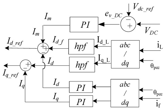
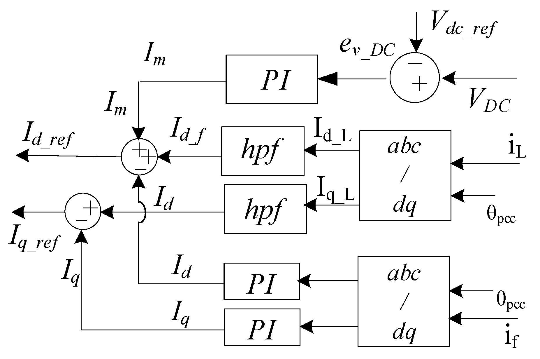
Figure 3.
Harmonic current control of shunt active filter [21].
Figure 3.
Harmonic current control of shunt active filter [21].
The load current (IL) is measured in real time and passed through a high-pass filter to isolate the harmonic components, effectively removing the fundamental frequency component. This filtered current represents the distortion and reactive components that need to be compensated for by the SAF. Concurrently, the current flowing through the SAF (If) is also measured and processed through another PI controller. This controller adjusts the filter current to minimize the error in the desired compensation current, further enhancing the system’s performance. Both the load current and the filter current are then transformed into the synchronous reference frame using a Park transformation. This transformation simplifies the control process by converting the three-phase currents into two orthogonal components. The dq components of the filter current (IFdq) are subtracted from the dq components of the load current (ILdq) to yield the dq components of the reference current that the SAF needs to inject to compensate for the harmonic and reactive components. This resultant dq reference current is then used to generate the modulation signals required for the inverter of the SAF, ensuring that the inverter injects the correct compensating current back into the system. This SAF control strategy dynamically compensates for harmonics.
3. Design of Shunt Active Filter Parameters
The first step in designing an effective SAF is to determine the load current and its harmonic components. This is achieved through fast Fourier transform analysis, which identifies the magnitude and order of the harmonics present in the load current. The harmonics directly influence the rating of the SAF, which must be capable of compensating for these harmonic currents. A safety margin of 25% is added to the calculated rating to ensure robustness and accommodate potential variations in harmonic content. The design assumptions include a voltage ripple of 6% and a current ripple of 10% [22,23,24]. The following calculations are performed for a rated loading condition of 1000 kW, where the power S can be expressed as (19) to get the current and voltage at the output of the load.
The relationship between the DC output current and the RMS value of the input AC current for a three-phase full-wave rectifier is given by:
is the RMS value of the per-phase input current.
The fundamental component of the non-linear load input current can help to find the current harmonic components.
The rating of the SAF can be obtained by (23). To account for dynamic conditions and ensure robustness, add a 25% safety margin to the calculated rating, i.e., 250 kVA.
The next step involves calculating the appropriate DC link voltage, which is determined based on the rated load conditions (24). This voltage must be sufficient to allow the SAF to inject the necessary compensating currents at the peak grid voltage. The modulation index (m) ranges from 0 to 1 and adjusts based on the load conditions. As the load increases, the m also increases, and vice versa. The m is typically considered 1 to accommodate a wide loading range for the SAF. The DC link voltage is calculated to 980 V; however, 1000 volts is considered for safety and adaptability.
VDC is considered 1000 V. The required capacitance for the DC link capacitor is calculated using the energy balance equation for capacitors. It considers the energy storage required to maintain the DC link voltage within the specified ripple limits during operation.
where ΔE represents the energy change, CDC is the DC link capacitance, VDC is the DC link voltage, and ΔVDC is the voltage ripple.
Here, ‘a’ is an overloading factor (a = 1.2), and k is the design coefficient (0.01) that normalizes the factors, t is the time by which DC bus voltage is to be recovered (0.03 s).
The series inductor, which links the SAF to the grid, is then designed. The inductance value is calculated based on the DC link voltage, current ripple, and the inverter’s switching frequency (27). The numerator accounts for the peak voltage across the inductor, which is influenced by the DC link voltage and modulation index. The denominator relates to the peak-to-peak current ripple Icr, which depends on the switching frequency fs. The remaining are the design constants to normalize the factors.
This inductor must be capable of handling the maximum current without saturating and should exhibit low losses to ensure efficient operation. Comprehensive simulation studies are performed to validate the design and ensure the SAF performs well under various operating conditions. Based on the test results, any necessary adjustments to control parameters and components can be made, ensuring the SAF operates optimally.
4. Results and Discussion
Table 1 presents the integrated power system network simulation parameters. The simulation was initially run without the SAF. After 1 s, the SAF was activated. The dynamic non-linear load was applied and varied from 100 kW to 800 kW.

Table 1.
Simulation parameters.
Figure 4 shows the power distribution in a power system over time, focusing on grid, load, inverter power, and the power absorbed by the SAF. The figure emphasizes the system’s response to an increase in load demand and the subsequent stabilization of power flows. Initially, the power flow is observed without the SAF. The SAF power initially showed significant fluctuations at 1 s due to its initial adjustment to the system’s harmonic and power requirements. The power is absorbed by an SAF over time, starting with zero power absorption before being activated. The figure also shows that the filter experiences transient power losses when activated and responding to sudden changes in load, but these losses stabilize over time. However, the SAF power loss is almost insignificant for the studied system. At 1.5 s, the grid is isolated, transitioning the system to GFM operation. From this point onward, the inverter solely supplies the load power and compensates for any additional power losses during the period of grid disconnection. At 2 s, the load was increased by 25%. The GFM successfully meets the load requirements. Despite this substantial increase in the inverter’s power supply to the load, the SAF consumes approximately 1% of the source power, which equates to about 8 kW. This underlines the SAF’s efficiency in managing increased load conditions with minimal additional power consumption.
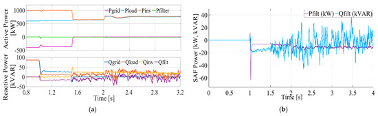
Figure 4.
Active and reactive power at different components of the system. (a) Active and reactive power in the network; (b) Active filter power loss.
The DC link voltage stabilizes near its reference value after the SAF is activated, ensuring the reliable operation of the inverter within the specified ripple band. It is shown in Figure 5a. The current through the DC link remained within acceptable limits, indicating that the inverter and the SAF functioned correctly without overstressing the power electronic components. Frequency variations were noted during the transitions when the SAF was connected. These frequencies quickly settled near the nominal value of 50 Hz, with the transient behavior expected during such transitions, as shown in Figure 5. The quick frequency stabilization indicates effective control within the inverter and SAF systems.
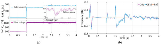
Figure 5.
System frequency and filter voltage and current characteristics. (a) SAF DC link voltage and current; (b) Inverter and grid frequency.
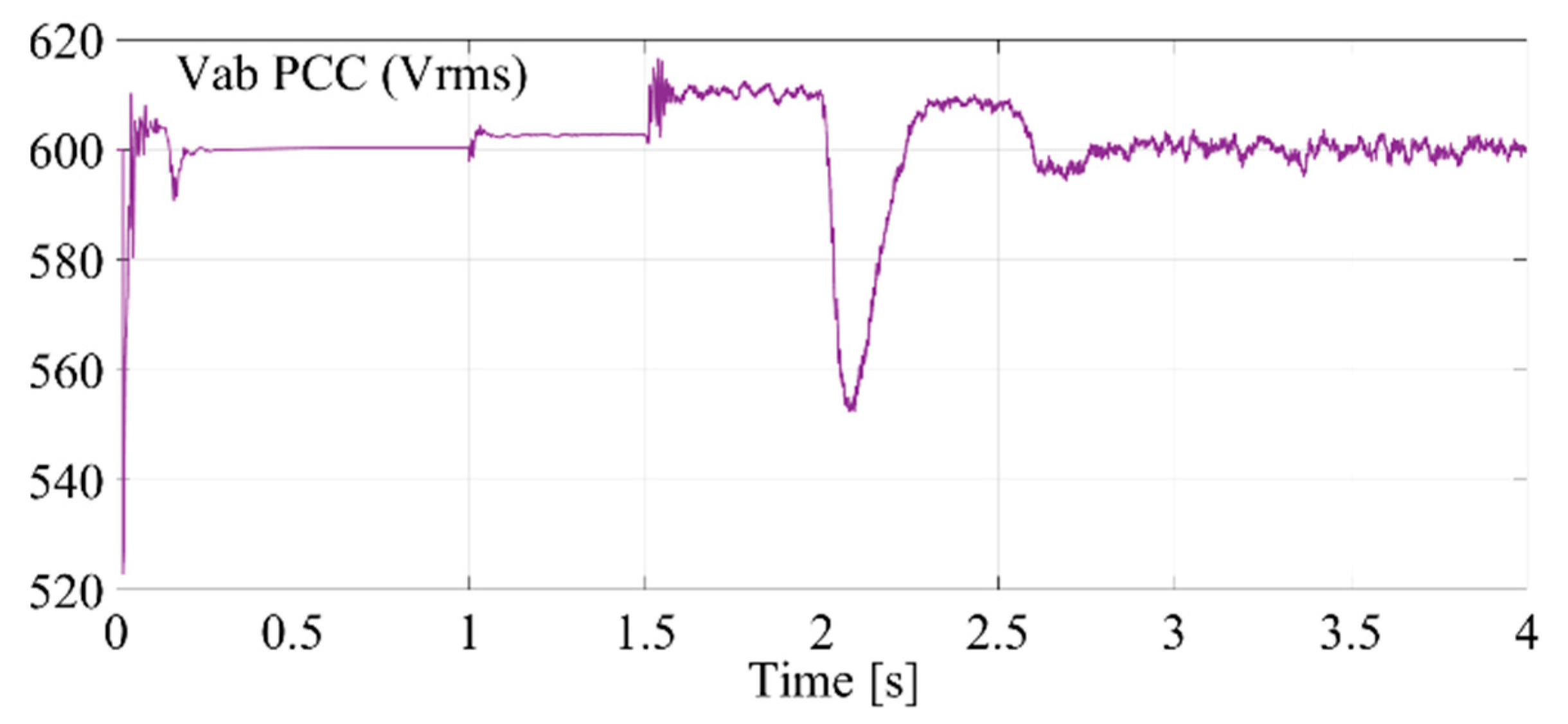
Figure 6 illustrates the voltage at the PCC over time, with key events highlighted. Before 1 s, the system was operating without the SAF, maintaining a stable voltage around 600 Vrms. At 1 s, the SAF activates, causing a slight disturbance but stabilizing the voltage. At 1.5 s, the grid is isolated, and the system switches to GFM, causing a significant disturbance or dip in the PCC voltage. At 2 s, the PCC voltage dips significantly due to an increase in load, and the inverter adjusts to provide additional power. After 2.5 s, the voltage stabilizes again, indicating that the GFM inverter has adapted to the new load conditions.
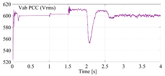
Figure 6.
Voltage at PCC in different operating conditions.
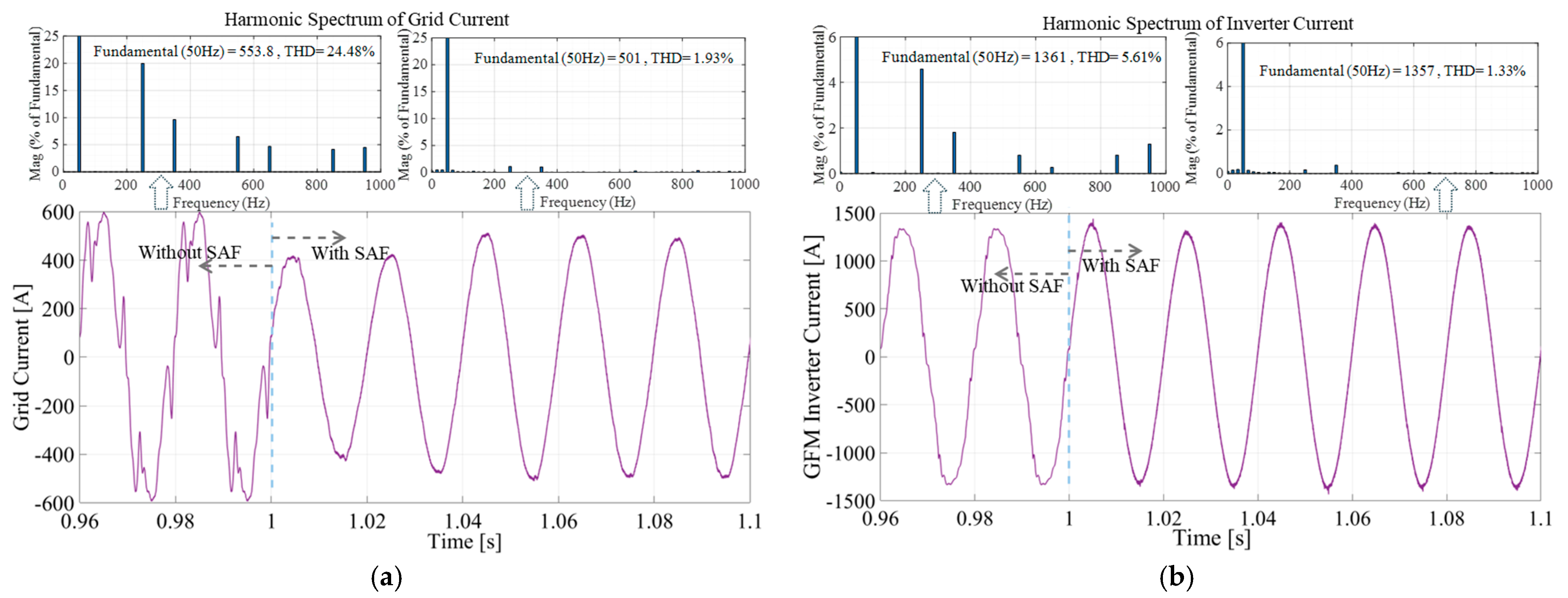
The harmonic spectrum analysis revealed significant improvements in power quality. Before the SAF was connected and the load was 600 kW, the THD in the grid current was 24.4%. After SAF activation, the THD reduced significantly to 1.93%, indicating that the SAF effectively filtered out harmonics from the grid current. Similarly, the THD in the inverter current dropped from 5.61% to 1.33% after the SAF was activated, showing that the inverter in conjunction with the SAF produces a better sinusoidal current adhering to IEEE standards. These results are shown in Figure 7.
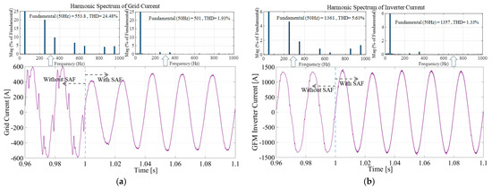
Figure 7.
(a) Grid current with harmonic spectrum without and with SAF; (b) Inverter current with harmonic spectrum without and with SAF.
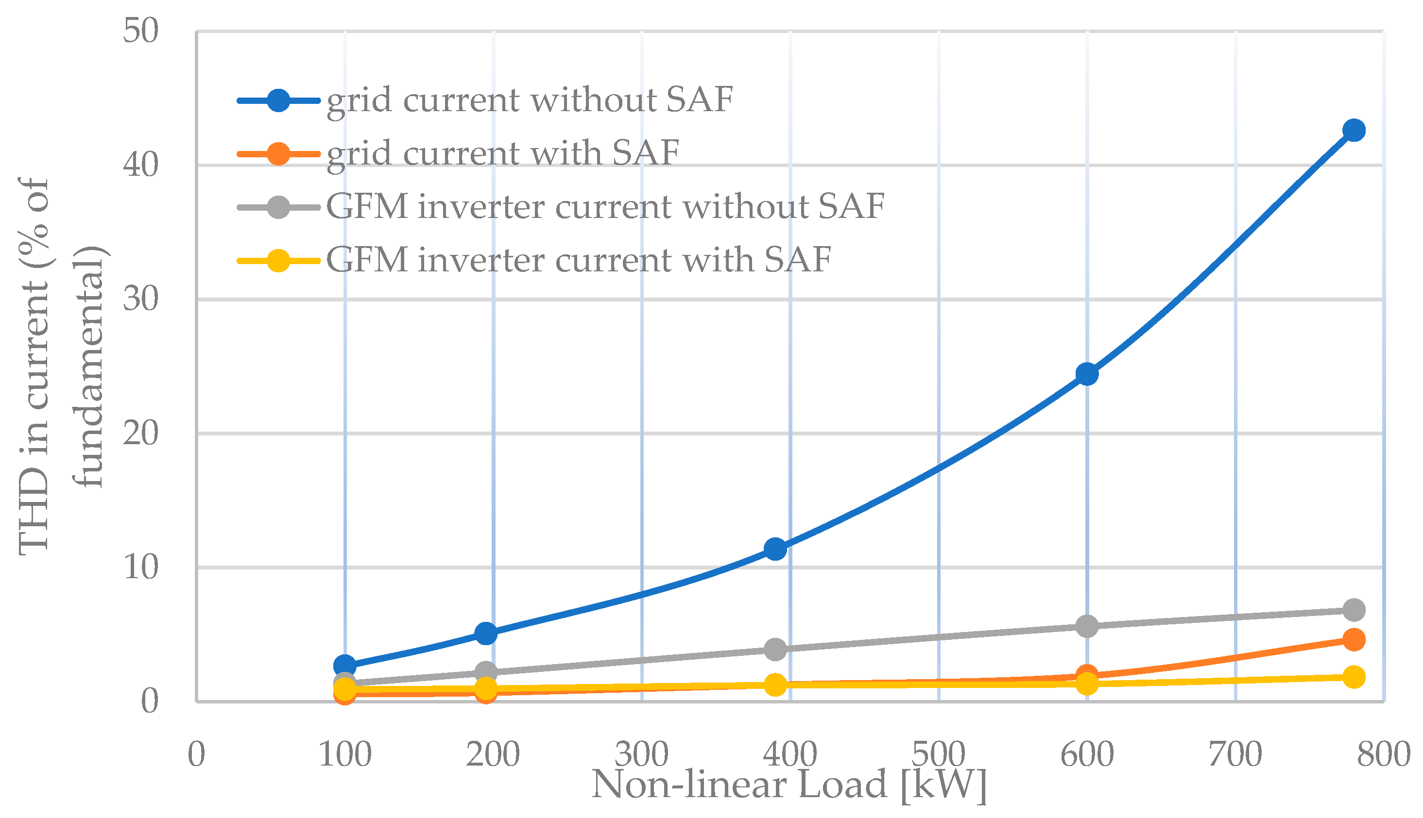
Figure 8 shows THD in the current under different operating conditions, with nonlinear loads ranging from 100 kW to 800 kW. The system’s performance is compared in four scenarios: grid current without an SAF, grid current with an SAF, GFM inverter current without an SAF, and GFM inverter current with an SAF. The first scenario shows a significant increase in THD as the nonlinear load increases, due to the grid’s inability to mitigate harmonics introduced by nonlinear loads. When the SAF is active, THD decreases across the entire load range, effectively compensating for nonlinear load harmonics.
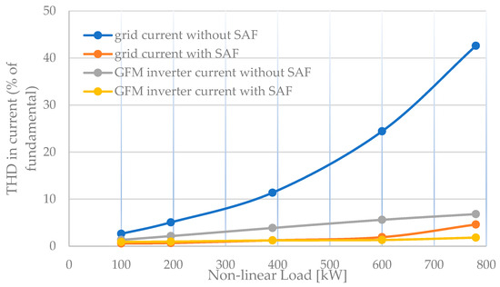
Figure 8.
Total harmonics distortion (THD) at different operating conditions.
For the GFM inverter current without the SAF, the THD is notably lower than the grid current without filtering, demonstrating the inherent ability of the GFM inverter to handle some level of harmonics. The rise in THD with load is more gradual, staying below 10% even at higher loads, reflecting the inverter’s partial compensation of harmonic distortions through its control strategies. Finally, the combination of the GFM inverter and the SAF results in minimal THD, which remains consistently low across the entire range of nonlinear loads, staying below 5%. This demonstrates the synergistic effect of the GFM and SAF in effectively reducing harmonic distortions, leading to optimal current quality.
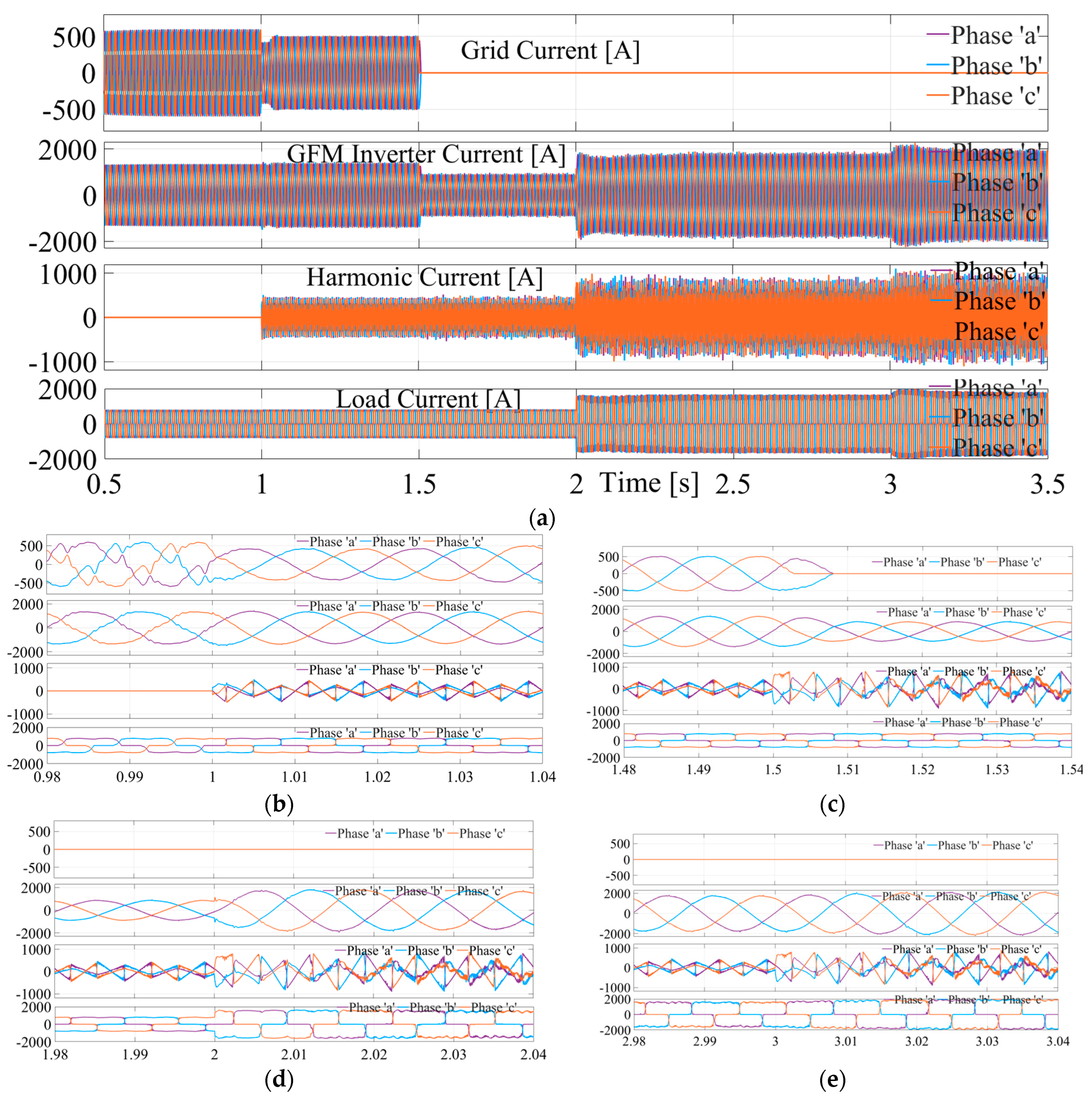
Figure 9 shows current waveforms for various nonlinear loads, sudden large load changes, and power grid failures to assess the performance and adaptability of the control strategy under realistic conditions. The system parameters remained unchanged except for load variations. To simulate a drastic load change, the load was increased by 200%, and a DC machine load was added, introducing another nonlinear element. The sequence of simulation events unfolds as follows: From 0 to 1 s, the inverter runs in grid-following mode, supplying a non-linear load of almost 750 kW. At 1 s, the shunt active filter is connected to mitigate harmonic distortions. At 1.5 s, a fault occurs, the grid isolates and the inverter switches to grid-forming mode. At 2 s, the non-linear load is doubled to reflect a drastic load change.
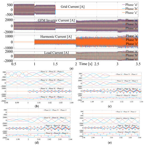
Figure 9.
(a) Power system network currents with and without shunt active filter. (b–e) Zommed-in view of power system network currents at different time.
At 3 s, the load is further increased by connecting a DC motor. This simulation effectively captures diverse operating conditions, including abrupt load changes, multiple non-linear load connections, and the transition to GFM mode following a grid failure. The inverter assumes control as the power source during the disconnection of the grid. The inverter’s current increases upon disconnection, demonstrating its ability to adapt to changing load conditions. The load current remains stable with a proportional increase when the load is doubled at 2 s. At 3 s, the addition of the DC motor causes a further increase in load current, confirming the introduction of additional load into the system. The inverter’s adaptive response to maintain system performance amidst fluctuating loads is demonstrated through the inserted plots. The figure highlights the inverter’s critical role in managing power quality and load demands effectively. Thus, the figure visually supports the description of the system’s response to sudden load changes, grid disconnection, and the involvement of multiple non-linear loads while highlighting the role of the shunt active filter in mitigating harmonic distortion.
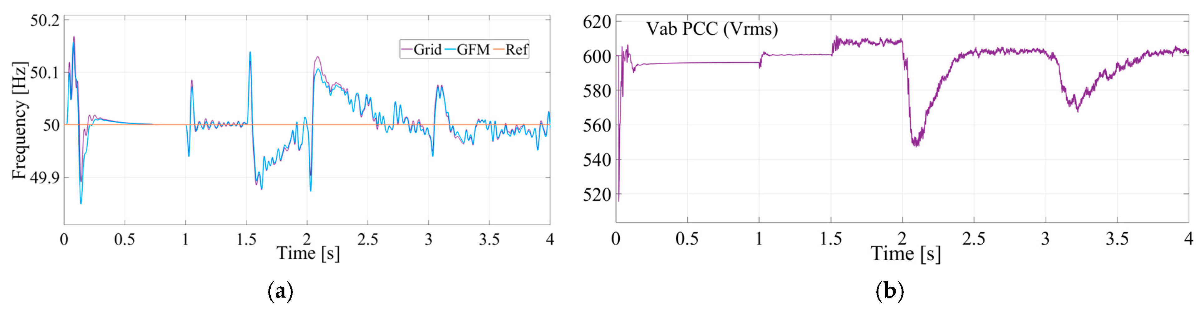
Figure 10 illustrates the system frequency dynamics, depicting how the frequency behaves during the transitions between the grid-connected mode and the grid-forming inverter mode, as well as during load changes. The system frequency response in a grid-connected operation is stable around 50 Hz, with minor oscillations. At 2 s, a temporary deviation from 50 Hz occurs as the load is doubled. After the load change, the system stabilizes again but with increased fluctuations compared to the pre-load change period. At 3 s, a further frequency deviation occurs when a DC motor is powered. Over time, the frequency stabilizes again. The inverter successfully handles frequency regulation in GFM mode, but the frequency is more sensitive to disturbances after grid disconnection, especially during large load changes. Figure 10b shows the voltage at the PCC. A significant drop at 2 s suggests a large disturbance due to a sudden load change. The voltage recovers and gradually returns to 600 Vrms. However, minor fluctuations persist, possibly due to residual system instability.
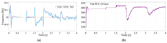
Figure 10.
Characteristics under drastic load change and high harmonic environments. (a) Inverter and grid frequency; (b) Voltage at PCC.
The constraints of control parameters for harmonics in a GFM inverter fed-system with an SAF are critical in ensuring effective harmonic mitigation while maintaining system stability and efficiency. The inductance of the filter is one such parameter with clear boundaries. On the lower end, if the inductance is too low, the filter may fail to sufficiently attenuate harmonic currents, leading to poor harmonic compensation and a higher ripple in the system’s current, which can stress the inverter’s switching components. Conversely, if the inductance is too high, the filter may become large, heavy, and costly, while also limiting its responsiveness to high-order harmonics, which can compromise the system’s ability to adapt to changes in harmonic content quickly. Similarly, a lower value for the DC link voltage would mean that the SAF inverter might not have sufficient voltage to generate the necessary compensating currents, especially for higher-order harmonics, thus reducing the effectiveness of harmonic cancellation. On the other hand, an excessively high DC link voltage can stress the inverter components and lead to higher energy losses, which can reduce the overall efficiency of the system. The switching frequency of the inverter is another key parameter with clear boundaries. A low switching frequency might not provide the necessary resolution for accurate harmonic compensation, leading to residual harmonic distortion in the grid current. However, if the switching frequency is too high, it can increase the losses and thermal stress on the inverter components, potentially leading to reliability issues over time.
Each of these control parameters must be carefully bounded to ensure that the SAF can effectively mitigate harmonics without compromising the overall performance and reliability of the grid-connected inverter system. Balancing these boundaries is key to achieving optimal harmonic compensation, system stability, and operational efficiency.
Limitations of Shunt Active Filters
Despite mitigating harmonics and improving power quality in grid systems, the SAFs face several limitations that impact their effectiveness. One of the primary challenges is their limited harmonic compensation capability in high-impedance grids. Their limited filtering bandwidth restricts the mitigation of higher-order harmonics, leading to residual harmonics that can distort the GFM inverter’s output. GFMs are commonly deployed in environments with weak or high-impedance grids, such as microgrids or remote locations. In these scenarios, the SAF’s ability to mitigate harmonics diminishes because the high grid impedance can lead to voltage distortions that the SAF struggles to compensate for effectively.
SAFs also face challenges with scalability and integration in grid-forming systems. Integrating an SAF can be complex in larger or more complex grid-forming applications, where multiple inverters are operating in parallel or in coordination with other distributed energy resources. The SAF must be carefully tuned to avoid conflicts with the GFM’s control system. Misalignment between the SAF and the GFM can lead to operational issues, such as circulating currents, resonance, or instability in the power network. Moreover, SAFs have constrained power ratings, which may result in overloading and inadequate harmonic compensation when exposed to higher harmonic currents, particularly in high-impedance scenarios. This inadequacy can compromise voltage control and increase sensitivity to load variations.
Furthermore, the inherent reactive power control limitations of SAFs pose challenges in GFM applications. Grid-forming inverters often need to manage both active and reactive power to ensure grid stability, especially in islanded or weak grid scenarios. SAFs, however, are typically designed to focus on harmonic compensation and may have limited capability to contribute to reactive power control. This limitation can be problematic in maintaining voltage stability and managing power flows in grid-forming applications, where reactive power control is crucial. To effectively utilize SAFs in GFM inverter systems, these limitations must be addressed through careful system design, advanced control strategies, and consideration of the specific operating environment.
5. Conclusions
The paper proposes a method for controlling the source current harmonics from integrated grid-forming inverters in modern power systems, offering a promising opportunity to enhance power quality, particularly when addressing the challenges posed by non-linear loads. This study has developed and analyzed harmonious modeling and control for integrated networks, incorporating voltage-source active filters. Shunt active filters effectively reduce harmonics from source current and ensure regulatory compliance by mitigating harmonics to acceptable levels. For instance, at a 600 kW load, the THD in grid current is reduced from 24.4% to 1.93% and remains within the standard despite increasing load in the linear range. The control maintains the power balance at the PCC for different loading and unloading conditions. Despite various transitions and operating conditions, the GFM operation maintains the frequency near the nominal value. These performance improvements support the reliable integration of renewable energy sources, reducing dependence on fossil fuel-based power generation and contributing to lower greenhouse gas emissions. Moreover, the adaptability and robustness of the SAF control system across various operating conditions make it well-suited for modern, dynamic grids, further supporting the transition to sustainable energy systems. The successful harmonic elimination and reliable performance demonstrated in this study highlight the critical role of advanced filtering and control techniques in achieving more efficient, resilient, and environmentally sustainable power networks.
Author Contributions
Conceptualization, J.H., K.R. and T.S.U.; methodology, K.R.; software, K.R. and D.O.; validation, T.S.U., H.K. and K.K.; writing—original draft preparation, K.R. All authors have read and agreed to the published version of the manuscript.
Funding
This paper is based on results obtained from the project, JPNP22003, commissioned by the New Energy and Industrial Technology Development Organization (NEDO).
Institutional Review Board Statement
Not applicable.
Informed Consent Statement
Not applicable.
Data Availability Statement
All relevant data supporting the findings of this study are available within the article.
Conflicts of Interest
The authors declare no conflict of interest.
References
- Benzaquen, J.; Miranbeigi, M.; Kandula, P.; Divan, D. Collaborative Autonomous Grid-Connected Inverters: Flexible grid-forming inverter control for the future grid. IEEE Electrif. Mag. 2022, 10, 22–29. [Google Scholar] [CrossRef]
- Matevosyan, J.; Badrzadeh, B.; Prevost, T.; Quitmann, E.; Ramasubramanian, D.; Urdal, H.; Achilles, S.; MacDowell, J.; Huang, S.H.; Vital, V.; et al. Grid-Forming Inverters: Are They the Key for High Renewable Penetration? IEEE Power Energy Mag. 2023, 21, 77–86. [Google Scholar] [CrossRef]
- Rahman, K.; Hashimoto, J.; Orihara, D.; Ustun, T.S.; Otani, K.; Kikusato, H.; Kodama, Y. Reviewing Control Paradigms and Emerging Trends of Grid-Forming Inverters—A Comparative Study. Energies 2024, 17, 2400. [Google Scholar] [CrossRef]
- D’silva, S.; Zare, A.; Shadmand, M.B.; Bayhan, S.; Abu-Rub, H. Towards Resiliency Enhancement of Network of Grid-Forming and Grid-Following Inverters. IEEE Trans. Ind. Electron. 2024, 71, 1547–1558. [Google Scholar] [CrossRef]
- IEEE Std.519-1992; Recommended Practices and Requirements for Harmonic Control in Electrical Power Systems. IEEE: New York, NY, USA, 1993; pp. 1–112. [CrossRef]
- Singh, B.; Al-Haddad, K.; Chandra, A. A review of active filters for power quality improvement. IEEE Trans. Ind. Electron. 1999, 46, 960–971. [Google Scholar] [CrossRef]
- Akagi, H. New trends in active filters for power conditioning. IEEE Trans. Ind. Appl. 1996, 32, 1312–1322. [Google Scholar] [CrossRef]
- Akagi, H. Active Harmonic Filters. Proc. IEEE 2005, 93, 2128–2141. [Google Scholar] [CrossRef]
- Akagi, H.; Watanabe, E.H.; Aredes, M. Shunt Active Filters. In Instantaneous Power Theory and Applications to Power Conditioning; IEEE: New York, NY, USA, 2017; pp. 111–236. [Google Scholar] [CrossRef]
- Chang, G.W. A new method for determining reference compensating currents of the three-phase shunt active power filter. IEEE Power Eng. Rev. 2001, 21, 63–65. [Google Scholar] [CrossRef]
- Budak, A.; Zeller, E.R. Practical design considerations for a variable center frequency, constant bandwidth, and constant peak-value active filter. IEEE J. Solid-State Circuits 1972, 7, 308–311. [Google Scholar] [CrossRef]
- Rahman, S.; Khan, I.; Rahman, K.; Al Otaibi, S.; Alkhammash, H.I.; Iqbal, A. Scalable Multiport Converter Structure for Easy Grid Integration of Alternate Energy Sources for Generation of Isolated Voltage Sources for MMC. Electronics 2021, 10, 1779. [Google Scholar] [CrossRef]
- EPRI. Grid Forming Inverters: EPRI Tutorial; EPRI: Palo Alto, CA, USA, 2021. [Google Scholar]
- Akagi, H.; Watanabe, E.H.; Aredes, M. Combined Series and Shunt Power Conditioners. In Instantaneous Power Theory and Applications to Power Conditioning; IEEE: New York, NY, USA, 2017; pp. 313–430. [Google Scholar] [CrossRef]
- Corasaniti, V.F.; Barbieri, M.B.; Arnera, P.L.; Valla, M.I. Hybrid Active Filter for Reactive and Harmonics Compensation in a Distribution Network. IEEE Trans. Ind. Electron. 2009, 56, 670–677. [Google Scholar] [CrossRef]
- Li, J.; He, Y.; Xu, L.; Liu, J. Design of Hybrid Power Filters for Harmonics Suppression in Power Electronics Dominated Power Systems. IEEE J. Emerg. Sel. Top. Power Electron. 2024, 12, 2163–2175. [Google Scholar] [CrossRef]
- Pan, Y.; Chen, L.; Lu, X.; Wang, J.; Liu, F.; Mei, S. Stability Region of Droop-Controlled Distributed Generation in Autonomous Microgrids. IEEE Trans. Smart Grid 2019, 10, 2288–2300. [Google Scholar] [CrossRef]
- Hart, P.J.; Goldman, J.; Lasseter, R.H.; Jahns, T.M. Impact of Harmonics and Unbalance on the Dynamics of Grid-Forming, Frequency-Droop-Controlled Inverters. IEEE J. Emerg. Sel. Top. Power Electron. 2020, 8, 976–990. [Google Scholar] [CrossRef]
- EGIS. Grid-Forming Technology in Energy Systems Integration; Energy Systems Integration Group: Reston, VA, USA, 2022. [Google Scholar]
- Xue, L.; Mu, L.; Fang, C.; Zhu, J. Research on Active Protection Method for Microgrids Based on Harmonic Injection. IEEE Trans. Smart Grid 2024. early access. [Google Scholar] [CrossRef]
- Tang, Y.; Loh, P.C.; Wang, P.; Choo, F.H.; Gao, F.; Blaabjerg, F. Generalized Design of High-Performance Shunt Active Power Filter with Output LCL Filter. IEEE Trans. Ind. Electron. 2012, 59, 1443–1452. [Google Scholar] [CrossRef]
- Aredes, M.; Hafner, J.; Heumann, K. Three-phase four-wire shunt active filter control strategies. IEEE Trans. Power Electron. 1997, 12, 311–318. [Google Scholar] [CrossRef]
- Rockhill, A.A.; Liserre, M.; Teodorescu, R.; Rodriguez, P. Grid-Filter Design for a Multimegawatt Medium-Voltage Voltage-Source Inverter. IEEE Trans. Ind. Electron. 2011, 58, 1205–1217. [Google Scholar] [CrossRef]
- Shyu, K.K.; Yang, M.J.; Chen, Y.M.; Lin, Y.F. Model Reference Adaptive Control Design for a Shunt Active-Power-Filter System. IEEE Trans. Ind. Electron. 2008, 55, 97–106. [Google Scholar] [CrossRef]


Disclaimer/Publisher’s Note: The statements, opinions and data contained in all publications are solely those of the individual author(s) and contributor(s) and not of MDPI and/or the editor(s). MDPI and/or the editor(s) disclaim responsibility for any injury to people or property resulting from any ideas, methods, instructions or products referred to in the content. |
© 2024 by the authors. Licensee MDPI, Basel, Switzerland. This article is an open access article distributed under the terms and conditions of the Creative Commons Attribution (CC BY) license (https://creativecommons.org/licenses/by/4.0/).