Abstract
The significance of the transportation sector, notably in terms of the carbon emission factor, is an undeniable fact. Along with this fact, individuals’ transportation preferences depend on their income levels. In this context, when the issue is considered, the income level in the USA pushes people toward cheap air travel. The main reason for this is that it is cheap, accessible, and transports one to their destinations quickly. Thus, from the perspective of road transportation, bus transportation is popular among the public. The reason why both air and road transportation modes are empirically evaluated together through income distribution is due to the preference of the US people. In this context, the effectiveness of active transportation on both air and highways in the USA from 1975 to 2023 is investigated by taking into consideration the income distribution. Empirical findings obtained through the FMOLS, DOLS, CCR, and NARDL models demonstrate that all independent variables, including GDP, energy use, air transportation, and the Gini coefficient, affect carbon dioxide emissions. In addition, wavelet analysis is performed to comprehend the form of and fluctuations in the series, which are vital to monitoring the periodical changes.
1. Introduction
In recent years, a lot of empirical research has been conducted to explain the linkage between environmental degradation and per capita income. The change in the production structure and its mass scale brought environmental destruction through the industrial revolution. Global warming, climate change, environmental pollution, and combating these problems have become important issues on the world’s agenda, with the increase in environmental destruction and the difficulties of controlling it. The interest in environmental problems and their economic effects in the economic literature has increased under the influence of the environmental issues developed by Grossman and Krueger [1].
Transportation, which is in the category of the services sector, has historically been as important as food, nutrition, shelter, security, and similar basic needs for national economies. Transportation can be described as the movement of living and non-living entities from one place to another economic perspective, it can be described as a service that enables all kinds of living and non-living entities to change places in a way that benefits from time and space in order to meet human needs. From this point of view, transportation can also be defined, in general, as a service element that benefits from time and space in the transportation of commodities, services, and people from one point to another. Transportation services consist of road, rail, sea, air, and pipeline transportation [2].
The economic dimension of transportation in terms of environmental issues is related to the use of scarce resources. It is expected that through the orderly distribution of scarce resources, there will be an increase in the consumption of goods and services and support economic growth. For this reason, the environmental dimension focuses on preserving the integrity and flexibility of ecological systems and the systems that support them as well [3].
The increase in greenhouse gas emissions in the world has also led to an increase in concerns about global warming and climate change. The impact of the logistics sector on CO2 emissions, one of the main causes of climate change, has been determined as 13.1%. The logistics sector, which connects the market and clients, acts within the framework of the green logistics approach, producing products with less energy consumption and in a way that makes them easily recyclable and durable. This approach also prevents the release of more waste than the system can handle by consuming less energy during transportation [4]. Zaman and Shamsuddin [5] state that energy consumption continues to pollute and negatively affect the global environment without implementing green policies where cargo is restricted or other logistics services interfere with the process of controlling carbon emissions, which is a crucial cause of climate deterioration and global warming. It is also mentioned that if logistics companies adopt green practices, it is possible to decrease the detrimental influences on the environment by up to 80% during their operation.
The importance of the logistics sector, especially in terms of carbon emissions, is an irrefutable fact when considering the relationship among energy, GDP, and CO2 emissions. Along with this fact, individuals’ transportation preferences depend on their income levels. In this context, when the issue is considered, the income level in the USA pushes people toward cheap air travel. The main reason for this is that it is affordable, accessible, and one transports to their destination quickly. Thus, from the perspective of road transportation, bus transportation is less popular among the public. The reason why both air and bus transportation modes are empirically evaluated together through income distribution is due to this preference of the US people. In this context, the effectiveness of active bus transportation on both air and highways in the USA from 1975 to 2023 is investigated by taking into consideration the income distribution. Empirical findings obtained through the FMOLS, DOLS, CCR, and NARDL models demonstrate that both air transportation and the Gini coefficient affect carbon dioxide emissions as well. The novelty of this study lie in the use of environmental economics literature through the NARDL method in the USA, where air transportation significantly affected the carbon emissions compared to road transport from 1975 to 2023. While working on a similar problem, Hussain et al. [6] investigated whether economic development, transportation, environmental expenditure, and income inequality affect transportation carbon emissions for OECD countries. The panel time-series data period and cross-sectional autoregressive distributed lag method are used with 2000–2020 annual data. As a result of their research, income inequality, environmental expenditures, and green transportation were found to be negatively related to the transportation carbon emission coefficient. Timilsina and Shrestha [7] analyzed the potential factors affecting the growth of transport sector CO2 emissions in Asian countries by decomposing the annual emission growth into components representing changes in the fuel mix, modal change, and GDP per capita. It was found that GDP per capita, population growth, and changes in transportation energy intensity are the main factors driving the growth of transport sector CO2 emissions in the considered countries. Mraihi et al. [8] revealed that vehicle fuel intensity, vehicle density, GDP per capita, urbanized kilometers, and the national road network were the major drivers of changes in energy consumption in the road transport sector in Tunisia during the period 1990–2006. In the first part of this article, the subject is discussed in general terms, and an essential framework is drawn; in the second part, the relevant literature is reviewed; in the third part, analyses are given; and in the last part, empirical findings are interpreted, and some guidelines are provided to the US Government and policymakers.
2. Literature Review
Along with globalization, privatization and commercial activities are important factors in the evolution of the aviation market and the transformation of airports. The increase in air traffic, regional development, and urbanization in the regions where the airport is located, together with the effect of the fuel types used, cause an increase in emissions. Today, the majority of the world’s population lives in cities, and this value will constitute a large portion of the population of developing countries, such as 64%, in 2050. With industrialization, the production of painful industrial products has caused an expeditious rise in the amount of greenhouse gas emissions in developing countries’ economic growth rates. Therefore, it can be stated that there are linear or nonlinear relationships between the rise in per capita income and carbon emissions. The most important source of the problems experienced in the world is energy. This is a problem related to the acquisition and processing of fossil fuels, especially oil and coal. The most determining force of world politics is energy resources. However, powerful countries and the rich segments of these countries that want to access these resources are causing great harm to the poor. As a result of the excessive pollution caused by the use of oil and coal, people are deprived of their right to an unpolluted environment. Poor people and countries, who are not responsible for the pollution of the atmosphere in any way, are the ones who pay the heaviest price for this. When the relevant literature is examined, one of the pioneering studies, Ang [9], tries to explain carbon emissions by using per capita income and the square of per capita income. Within the framework of the empirical analyses conducted, Ang [9] reveals that the rise in per capita income reduces carbon emissions after a particular point. Particularly after the 2000s, the volumes of foreign trade in these countries increased in parallel with the rapid increase in income in developing countries. Accordingly, it is frequently examined in the literature that developments in the transportation and logistics sectors cause increases in carbon emissions. The findings of this paper are clearly parallel with the empirical results of Ang [9].
There are many studies conducted in the USA and other countries using variables such as GDP, energy usage, and CO2 emissions. Various analysis methods are used in the studies to scrutinize whether there is a relationship among certain variables. However, there is no study comparing variables, such as airlines, highways, and income distribution, and integrating them into the existence of the effects of both energy consumption and GDP on CO2 emissions. This study is important in terms of eliminating this deficiency in the academic literature. It is observed that in the environmental economics literature regarding transportation types, authors, such as Bahadir, Egilmez, Dursun, Bahadir, Kayabas, Yazici, Dursun, Kalayci and Yazici, Kalayci and Yanginlar, Ozkan et al., Kalayci and Artekin [10,11,12,13,14,15,16,17,18,19,20], have examined the carbon dioxide emissions by considering air, road and sea transportation, and ecology. In this sense, Kalayci and Koksal [21] employ the linear regression and Johansen cointegration model in order to test both the relationship and effect coefficient among the series from 1980 to 2011 for China.
When other academic studies on the linkage between the transportation sector and carbon emissions are examined, it is seen that there is little research dealing with airway and highway logistics in terms of environmental issues. If it is intended to make an observation on some studies, Manga [22] analyzes the relationship between the total output level of the transport market and the CO2 emissions produced by this sector using the Panel AMG method using the 1995–2016 period data of 22 OECD countries and showed that there is an inverted U-shaped nexus among relevant variables. Hassan et al. [23] examined the air transport market of 21 OECD countries by implementing the GMM method from 1980 to 2018. While an inverted U-shaped linkage is determined in the field of GDP and air travelers, U-shaped empirical findings are discovered in the field of airline freight transportation. In the Dumitrescu–Hurlin panel causality test, a unidirectional causality connection is revealed from economic growth to aviation sectors’ carbon emissions. Gyamfi et al. [24] investigated the air and rail transportation of E7 countries through panel data tests by employing data from 1995 to 2016. They determined that rail transportation and urbanization decrease environmental degradation. Therefore, it is emphasized that rail transportation should be encouraged, notably for a sustainable environment.
Ozkan et al. [19] scrutinized the influence of GDP and energy consumption on CO2 emissions by using data for the period 1980–2013 for eight developing and eight developed countries. The empirical findings obtained for the period 2001–2013 reveal the existence of environmental degradation. Erdogan et al. [25] tested the energy use and GDP on environmental degradation for the period 1995–2014 for the 10 countries with the most airline transportation. The findings demonstrate there is an impact of GDP and energy on CO2 emissions. Ozpolat [26] peruses the relationship between total, production, and transportation sector CO2 emissions and per capita income by controlling the effects of urbanization and energy use on emissions by implementing panel data tests. According to the findings attained from that study, there is an influence of economic growth and energy usage on carbon dioxide emissions. Hassan and Nosheen [27] examined the effect of air transport on greenhouse gas emissions, nitrogen emissions, and methane emissions for Pakistan between 1990 and 2017 by using three separate models. In this context, ARDL, Granger causality, and vector autoregression (VAR) are used by considering three dependent and seven independent variables. As a result, it was determined that there was a substantial and positive linkage among air transportation and carbon dioxide, nitrogen, and methane emission groups. It is also determined that GDP, population density, and energy demand had significant and positive effects on all three emission categories, and it is stated that they significantly affected the environment.
Danish et al. [28] scrutinized the nexus among energy use, economic growth, and CO2 originating from the logistics market in Pakistan from 1990 to 2015 by using ARDL and VECM models. As a result, they found that foreign direct investments contribute to CO2 emissions. They also found that the effect of GDP and urbanization on CO2 emissions originating from the transportation sector is statistically insignificant. Chatti [29] examined the relationship between information communication technologies, transportation (road, railway, and air), and CO2 using data from 43 countries between 2002 and 2014 by using the Generalized Method of Moments. As a result, they found that information communication technologies and freight transportation increase CO2, and the interaction between these two variables can improve environmental quality in terms of reducing carbon emissions. It is also stated that internet use is the most efficient technology in reducing CO2 emissions when interacting with air cargo transportation. Sohail et al. [30] demonstrated the asymmetric impact of air–rail transportation on environmental degradation in Pakistan for the period 1991–2019 using the ARDL model. As a result, they found that the number of airline passengers and the number of railway passengers increased carbon emissions. They stated that this result indicates that a 1% rise in the total number of passengers transported by air in Pakistan increased environmental pollution by 0.21% in the long run.
Law et al. [31] examined the long-run connection among GDP, air transport, and inbound tourism for Myanmar, Cambodia, Vietnam, and Laos (CLMV countries) in Southeast Asia in between 1995 and 2018 by implementing ARDL and Granger causality tests. As a result, they found two-way causality between GDP and air traffic in the long term. Shafique et al. [32] ascertained the link among environmental degradation, transportation, and economic growth in 10 Asian economies through the highest carbon dioxide emissions values for the period 1995–2017 using the ARDL model and the Dumitrescu and Hurlin causality test. As a result of the causality test, they found a one-way causality between transportation and economic growth and between transportation and environmental degradation. In addition, they concluded that there is an internal connection among transportation, CO2 emissions, and economic growth and stated that emissions and environmental degradation are mostly affected by economic growth and the transportation sector. Habib et al. [33] investigated the effect of air transport intensity, air passenger transport, and air cargo transport on carbon emissions from air transport in G20 countries from 1990 to 2016 by performing panel quantile regression model and Dumitrescu and Hurlin causality tests. As a result, they found that the impact of air transport intensity, air passenger transport, and air cargo transport on carbon emissions is positive. They state that GDP, tourism, and urbanization are important contributing elements in increasing CO2 emissions from air transport. In the results of the causality test, they reveal that there is bidirectional causality from air transport intensity, air passenger transport, and air cargo transport to CO2 emissions from air transport.
Wang et al. [34] analyzed the carbon dioxide emissions intensity trends of 51 countries considering the Belt and Road by using the Theil model during 2000–2014. The research findings show that the CO2 emissions of the transport market and output value of several countries considering the Belt and Road have increased, but the CO2 emissions intensity shows an overall decline through a polarization trend. Yin et al. [35], in their study, developed a detailed model using the Global Change Assessment Model (GCAM) to assess the energy use and CO2 emissions of China’s transport market. The analysis predicts that without current policies, transportation energy and carbon dioxide emissions will increase, leaving the sector dependent on fossil fuels. Carbon pricing policies could reduce emissions, but their impact would be limited, they noted. Xu et al. [36] assayed the effects of economic growth and energy usage on carbon dioxide (CO2) emissions in the United States between 1981 and 2018 using the wavelet technique, with evidence from the transportation sector. According to findings, non-renewable energy use has a tremendous effect on CO2 emissions in the short, medium, and long term; renewable energy has a positive effect on CO2 emissions in certain stages in the short term, and economic growth has a substantial effect on CO2 in the long and medium term. In addition, Okanli and Demir [37] stated that the carbon footprint in urban areas in Türkiye may be high depending on factors, such as energy consumption, transportation, consumption habits, and waste management. However, it is possible to reduce the carbon footprint in urban areas with strategies, such as energy efficiency, use of renewable energy sources, sustainable transportation, and recycling. City administrations and individuals can contribute to a more sustainable future by implementing these strategies If a separate issue is considered in terms of the impact of highways on carbon emissions, notably, Onder and Kaya [38] state that technology leadership in sector like electric vehicles will become the transportation technology of the future. The authors demonstrate that a country can achieve sustainability, competitive advantage, and increase export potential in related industries by succeeding in leadership in electric vehicle technology. Policymakers can support sustainable technological transformation by encouraging domestic electric vehicle production. Economic and political reasons are important factors to encourage the transition from fossil fuel use to electric vehicles in the automobile sector. However, supporting policies, such as infrastructure development, financial incentives, regulatory measures, and awareness-raising efforts, to ensure consumer acceptance should also be implemented during this transition process. Moreover, Pradhan et al. [39] demonstrated that there are stable endogenous relationships among the variables in the short and long term in developing economies. Furthermore, CO2 emissions can be reduced by ensuring greater use of renewable energy to power the transport sector. Consequently, a more environmentally friendly transport sector, including the highway, airway, and maritime sectors, will be critical in enabling these countries to transition to sustainable economic growth trajectories.
3. Methodology and Data Analysis
The main objective of this study is to reveal whether highway and air transportation along with income distribution had a positive or negative effect on carbon emissions between 1975 and 2023 in the USA. In this context, whether the long-term impact coefficient is positive or negative is tested through the NARDL method. There is no other research paper in the academic literature on environmental economics that compares transportation types with income distribution. In this respect, this study can be considered to make a noteworthy contribution to the academic literature.
Firstly, datasets related to variables are obtained from official websites in order to perform unit root and NARDL analyses. In this sense, datasets for air transportation, GDP, and Gini coefficient are derived from the official website of the World Bank [40,41,42]. In addition, carbon emissions and energy consumption are gathered from the authorized website of Our World in Data [43,44] and included in the research model as well. Finally, statistics on American highways are collected from the Federal Highway Administration [45] database. Missing datasets of Gini and airline transportation for 2022 and 2023 are obtained from some official websites, such as BTS [46], STATISTA (2024) [47], and United States Census Bureau [48]. The dataset regarding the variables of this article is up to date and in the broadest scope. The beginning year of this study is determined as 1970 in order to cover this period with the acceleration of trade volume in the USA. Datasets related to all variables are determined to be greater than 30 for a parametric test. In addition, all variables’ logarithm and GDP square are taken to perform both unit root and NARDL tests. Additionally, CO2 emissions are designated as the dependent variable, and those remaining are designated as explanatory variables in the research model. In other words, all other variables are determined as exogenous variables.
After the stage of obtaining datasets regarding variables, generalized Dickey Fuller ADF (Augmented Dickey Fuller), PP (Phillips Perron), KPSS (Kwiatkowski–Phillips–Schmidt–Shin), ZA (Zivot-Andrews), and LS break unit root tests, Lee and Strazicich [49], are applied to determine the stationarity levels of the series. Null hypotheses consider that the relevant series is not stationary; in other words, it contains a unit root, which is proved through Dickey and Fuller [50] ADF and Phillips and Perron [51] PP unit root tests. The H0 hypothesis of the Zivot and Andrews [52] ZA test, which takes into account the possibility of structural breaks in the series, states that the relevant series contains a unit root. The H0 hypothesis of the LM break unit root test also claims that the relevant series contains a unit root. If the variance and mean of a time series do not change over time and the common variance between two periods does not depend on the period in which this common variance is calculated but only on the distance between the two periods, then the series is stationary [53]. In empirical analyses using time series, it is first necessary to test the stationarity of the series used in the model or whether there is a unit root. In studies, the Augmented Dickey Fuller (ADF) test is generally used to test the stationarity of variables. The ADF test includes the lagged values of the dependent variable in the model as an independent variable. Thus, in the error term with autocorrelation, the autocorrelation is eliminated with the lagged values of the time series. The number of lags is selected according to the Akaike and Schwarz information criteria. The following equations are used in the ADF test.
Equation with constant and without trend:
Constant-trend equation:
In the equations, “(Δ)” represents the first difference, “(Yt)” t represents the time series in the period, “()” represents the constant term of the series, the error term, the time trend, and (p) the lag length. In the ADF test, if the value of the result of the ordinary least squares method estimates is sufficiently negative or is smaller than the critical values, H0 is rejected, and the series becomes stationary.
The hypotheses of the Augmented Dickey Fuller (ADF) unit root test are as follows:
H0.
or
δ = 0 (There is a unit root, so the series is not stationary).
H1.
δ < 0 (There is no unit root, so the series is stationary).
Perron and Phillips [54] is another unit root test. Phillips and Perron used nonparametric statistical methods to eliminate the autocorrelation problem in the error terms. In this test, the statistics are transformed in order to eliminate the effect of autocorrelation on the asymptotic distribution of the test statistics. The critical values used in the DF test are also used in the PP test. The model developed by Phillips and Peron allows the error terms to be weakly dependent and heterogeneously distributed. Phillips Perron, unlike the ADF test, does not include the lagged values of the dependent variable in any equation. In unit root tests, a stationary series subject to a structural break may appear to be non-stationary. This situation may cause the null hypothesis to be falsely rejected in unit root tests where the structural break is not taken into account. For this reason, Perron [55] developed a unit root test that can be applied under the assumption of a single structural break known to be external. The Perron unit root test is based on the addition of the correction factor suggested by Perron [55] to the ADF process.
The Hypotheses H0 and H1 are used in the PP test.
The equations of the PP are demonstrated below. The PP test differs from the ADF test in that the error terms are not statistically independent, have a weak dependence between them, and show a heterogeneous distribution rather than a homogeneous distribution.
Equations (4) and (5) above show the fixed and fixed trend models, respectively. is the tested variable, is the constant term, t is the trend indicating the error term and the aggregate observations. The value calculated in the PP method is compared by the “MacKinnon” critical table to determine whether the series is stationary or not. It also indicates the value coefficient to be tested in this method.
Zivot and Andrews [52] criticized Perron’s [55] assumption of an exogenous breakpoint and developed a new unit root testing procedure that allows for an estimated break in the trend function under the alternative hypothesis. In the Zivot–Andrews (ZA) unit root test, three models are implemented: Model A permits a single break at the level, Model B permits a single break at the slope, and Model C permits a single break at both the level and the slope.
“DU” in the models is dummy variables representing the break in level and “DT” in slope.
Here, t = 1, 2, …, T is the time, represents the break date, and λ = TB/T gives the breakpoint.
First of all, for each series, Equations (6)–(8) are estimated by using the least squares method with the breakpoint “j = 2/T” and “j = (T − 1)/T” in the interval “λ = Tb/T”. For each “λ” value, the number of additional variables k is determined by the same procedure as Perron tests and is calculated for the test of “δ”. The break date is selected as the date with the smallest t statistic [52]. After the break date is determined, if the designated t statistic is smaller than the critical value calculated by Zivot and Andrews [52], the basic hypothesis expressing that there is a unit root is accepted as well. In the application of the ZA unit root test, the first model is estimated, and the appropriate model is selected according to the significance of the parameters of the dummy variables DU and DT. If both dummy variables, DU and DT, are statistically significant, Model C is appropriate; if only DU is significant, Model A is appropriate; and, finally, if only DT is significant, Model B is appropriate. There is no consensus on which of these three models is superior, but in practice, the first model and Model C are generally used. As in other unit root tests, this test is also sensitive to lag length. In the ZA unit root test, the rejection of the basic hypothesis indicates that CO2 is not stationary.
On the other hand, when Equations (9)–(11) below are examined in depth, the intercept dummy represents a change in the level; if (t > TB) and zero otherwise; the slope dummy (also refers to a change in the slope of the trend function; DT* = t − TB or () and zero otherwise; the crash dummy (DTB) = 1 if t = TB + 1 and zero otherwise; and TB is the break date. Each of the three models has a unit root through a break under the null hypothesis, as the dummy variables are incorporated in the regression under the null.
In this study, the NARDL (Nonlinear Distributed Lag Autoregressive Model), which was developed by Pesaran et al. [56] and is based on the ARDL bounds test, is employed to determine the asymmetric effect of the types of transportation and Gini coefficients on CO2 emissions. However, this model differs from the ARDL test by using the cumulative sums of both positive and negative shocks of the independent variables, and the long-term asymmetric relationship in the model is expressed as in Equation (12):
Here, β+ and β− are the long-term asymmetric parameters. + and are the positive and negative changes and are shown as follows:
The asymmetric effects of exchange rate ( and ) on CO2 emissions are estimated with the NARDL (p, q) model as in Equation (13):
Thus, η+ = −ρβ+, η− = −ρβ−, πi+ = −βφi+ + ψ2i, πi− = −βφi− + ψ2i i = 1, 2, …, p, q = p + 1.
4. Stages of NARDL Model
The Nonlinear ARDL model stages are as follows:
The main advantage of using NARDL compared to the other econometric models is that it allows the underlying variables of the study to shift over the period. It also includes an error correction process or mechanism that takes into account the asymmetries in the long-run cointegration. Moreover, it allows for asymmetric observations in both positive and negative responses to changes in carbon emissions. Therefore, NARDL is compatible with preserving the variables considered in developing a new structural analysis. As a result, this research closes the gap and provides concrete evidence for the USA. An important advantage of the NARDL model is that it can be applied regardless of whether the variables in the analysis are I(0) or I(1) [56,57]. At the same time, the NARDL method, which takes into account asymmetric effects, allows for cointegration analysis, regardless of whether the variables are zero or first-degree integrated [58]. Therefore, the ARDL method can be performed without the need for any stationarity test. However, if the variables in question become stationary in their second differences, since there are no critical table values for this situation, a unit root test must be performed to prove that the variables in the analysis are not I(2). Based on this, the first stage in the NARDL model is to perform a unit root test to determine the integrated degrees of the variables. In the second stage, Equation (13), which takes into account the asymmetric relationship in the short and long term, is estimated by the least squares method. Then, the long-run cointegration relationship between CO2, transportation t+ and transportation t+ is tested. For this, the alternative hypothesis H1 = p < 0 against the null hypothesis H0 = p = 0 is tested through the t-test (tBDM) put forward by Banerjee et al. [59] or the alternative hypothesis (H1: p ≠ η+ ≠ η− ≠ 0) against the null hypothesis (H0: p = η+ = η− = 0) is tested with the F test (FPSS) developed by Pesaran et al. [56]. Afterwards, the test statistics obtained as a result of these tests are performed according to Pesaran et al. [56], which are compared with the table values, and, finally, it is determined whether the series are cointegrated or not.
Finally, the existence of a symmetric relationship in the short and long term is tested using the Wald test. The existence of a long-term symmetric relationship is tested through the hypothesis H0: η+ = η− or (WLR: L+lntrns = L−lntrns) and the existence of a short-term symmetric relationship is tested with the hypothesis H0: πi + = πi− or (WSR: Σip = 0 = πi+ = Σpi=0π−i) (i = 0, …, p). Alternative hypotheses corresponding to the null hypotheses express the asymmetric relationship.
In addition to Equation (14) (Model 1), which assumes an asymmetric relationship in both the long and short term, there are three different equations depending on whether a symmetric relationship is accepted in the short and/or long term as a result of the Wald test:
It is assumed that there is an asymmetrical relationship for the long term and a symmetrical relationship for the short term with the equation in Model 2 above, a symmetrical relationship for the long term and an asymmetric relationship for the short term with the equation in Model 3, and, finally, a symmetrical relationship for both the long and short term with the equation in Model 5, which is the traditional linear ARDL model.
According to the approach developed by Shin et al. [58], when short-term and long-term asymmetries are added, the following NARDL models can be shown: In Equation (17), shown above, it can also be tested whether the exchange rate has an asymmetric effect on consumer prices in the long and short term. In Equation (17), as in the ARDL model, the λi parameters represent the short-term coefficients of the relevant variables and the αi parameters represent the long-term coefficients of the relevant variable. Short-term analysis aims to evaluate the short-term effects of changes in external variables on CO2 emissions.
5. Empirical Results
Examining the asymmetric effects of transportation types (air, highway), Gini coefficients, GDP, and energy consumption on carbon emissions, ADF, PP, KPSS, ZA, and LS unit root tests are used to test the variables in question, and the results of the relevant tests are shown in Table 1.

Table 1.
ADF, PP, KPSS, ZA, and LS unit root test results for the USA.
Based on the unit root test results in Table 1, it is concluded that there is a unit root problem in all variables due to the fact that the probability values in the ZA, ADF, PP, and LS test outputs regarding the level values of the variables are above 5%, and the test statistics in the KPSS test outputs are above the critical values. However, when the first difference of the series in analysis is assumed, it is seen that the probability values for the PP test are below 5%, and the KPSS test statistics are below the critical values. Therefore, the stationarity of the series after the difference taking process made it possible to perform the NARDL analysis. In other words, it has been observed that all the series in Table 1 above are stationary at the I(1) level and that the t-statistic values are at least higher than 5 percent.
Table 2 demonstrates the short- and long-term coefficient estimates of positive and negative shocks occurring in the asymmetric determinants of CO2 emissions. First of all, it is seen that the long-term elasticity coefficients (lnAR+ and lnAR−) associated with the positive and negative shocks occurring in air transportation are statistically significant at the 1% and 5% levels, respectively. Accordingly, irregular changes in Gini (negative shocks) and real value gains (positive shocks) create significant asymmetric effects on CO2 emissions in the long term. When the signs of the coefficients are examined, it can be said that the increase in air transportation causes environmental pollution by affecting it both positively and negatively. In fact, when energy consumption is considered, (lnEC+) and (lnEC−) affect it both negatively and positively. (lnGDP+), (lnGDP−) and (lnGINI+) also indicate that (lnGINI−) significantly affects the dependent variable, carbon dioxide emissions.
Table 2.
NARDL analysis of USA 1975–2023.
According to the NARDL long-term test results in Table 3, a 1-unit increase in energy consumption causes a 0.76-unit increase in carbon emissions, while a 1-unit decrease reduces carbon emissions by 0.95 units. A 1% increase in economic growth causes a 0.44-unit increase in carbon emissions. In addition, Cusum and Cusum’s graphs indicate how stable the model shown in Figure 1 and Figure 2 is. According to the Cusum and Cusum’s graphs in Figure 1 and Figure 2, it is seen that the model is stable, and no structural break is observed in the period subject to analysis. Asymmetry graphs of the variables used in the analysis are given in Figure 1 and Figure 2. In other words, in both graphs, the blue lines move between the two red lines without overflowing, which confirms the models.
Table 3.
Long-run NARDL forecast outcome of USA.
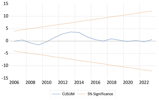
Figure 1.
CUSUM test of USA.
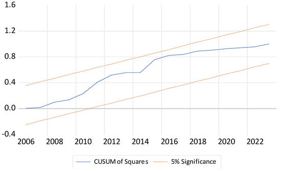
Figure 2.
CUSUMS test of USA.
The existence of an asymmetric cointegration relationship between variables is tested using the asymmetric bounds test in the first stage in the NARDL approach. Table 4 and Table 5 show the results of the asymmetric cointegration test conducted on the existence of a long-term asymmetric relationship between variables. According to Table 4 and Table 5, the F statistic is “14.0236”, which is above the upper critical limit of 3.680 at the 1% significance level. According to these results, the null hypothesis is strongly rejected for the model, and the existence of a long-term asymmetric and nonlinear relationship between variables is accepted, which verifies the model. Table 6 and Table 7, below, reveal the results of diagnostic tests for the NARDL model. Breusch–Pagan–Godfrey test results indicate that there is no autocorrelation and heteroscedasticity problem in the model, and Ramsey–Reset test results demonstrate that there is no error in the model specification. Finally, when viewing the FMOLS, DOLS, and CCR models in Table 8, below, it is seen that GDP, energy consumption, and air transportation affect carbon emissions. These empirical findings have contributed to the academic literature by overlapping with the results obtained in the NARDL model. Additionally, according to these models, there is a long-term relationship between the variables.
Table 4.
F and t statistics test of USA.
Table 5.
F bound test of USA.
Table 6.
Godfrey–Pagan–Breusch test for USA.
Table 7.
Ramsey reset test of USA.
Table 8.
FMOLS, DOLS and CCR of USA.
6. Wavelet Analyses: Application of Discrete Wavelet Transform Technique and Wavelet Outlier Detection for USA
The USA’s CO2 caused by air transport and energy use, GDP, and Gini fluctuates periodically. Wavelet analysis is applied to reveal them separately and interpret them empirically in terms of the USA’s CO2 emissions and air transportation, which are two major variables between 1975 and 2023 in Figure 3. Seasonality exists if fluctuations are of a constant frequency (that is, the frequency of fluctuations does not change) and are related to some aspect of time. If the fluctuations are not at a constant frequency, there is cyclicity.
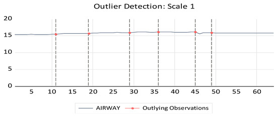
Figure 3.
Outlier detection of air transport for USA from 1975 to 2023.
In general, the average length of cyclical fluctuations is longer than the length of a seasonal pattern. The magnitude of cyclical fluctuations tends to be more variable than the magnitude of a seasonal pattern. That is, in cyclical fluctuations, the wavelength varies from period to period, whereas, in seasonal patterns, the wavelength is always more or less the same. In this context, wavelet outlier analysis can be employed for high-frequency and relatively more dynamic data. As a matter of fact, fluctuations in the natural gas needs have developed in countries such as the USA and are inevitable as well. When the wavelet outlier detection through scale two is applied to air transport, it is comprehended that the changes and fluctuations in this variable are much higher, notably in the earlier years (1978–2009). When the last ten years of air transport are examined in Figure 3, it is indicated that there is a relative stability. The most obvious reason why natural gas imports have become stagnant, especially in the last decade, is the increase in general conjuncture and costs. Thus, it has become inevitable for people in some suburban districts to turn to poor alternatives instead of expensive transportation modes, especially during the urbanization process. As shown in Table 2, the NARD model indicates that the impact coefficient of air transport is negative and positive on the CO2 and can be explained using the stagnant term in air transport, notably during the last 10 years.
The USA’s CO2 emissions were analyzed by using the discrete wavelet transform test (Figure 4). There were no major changes in terms of CO2 emissions in the 1980s. However, exceeding the threshold limit, which is a relative extremely sharp red line in the millennium and a sharp red line in the mid-2010s, can be explained by the radical increase in CO2 emissions. Notably, a decrease in the population growth rate and fertility rates has enabled the CO2 emissions to remain more stable and the recent periods in Figure 4 to remain stable in the USA during the last ten years.
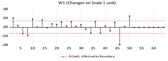
Figure 4.
Discrete wavelet transform analysis in terms of USA’s CO2 emissions (1975–2023).
7. Conclusions
In this study, empirical findings obtained through the FMOLS, DOLS, CCR, and NARDL models demonstrate that air transportation, GDP, energy use, and Gini affect carbon dioxide emissions. These results are consistent with the studies of Bozma [60], Hassan and Nosheen [61], and Hassan et al. [62]. Carbon emissions are of great importance in terms of environmental pollution and, most importantly, climate change. Within the scope of the Kyoto Protocol, countries are taking steps to reduce carbon emissions. In terms of the aviation sector, Switzerland, in particular, is implementing policies that will impose carbon emissions on consumers. In this context, carbon tax has taken its place in the first place in the country. In the USA, after the 1950s, there was a massive migration from rural to urban areas and rapid population growth, and the use of transportation vehicles has also increased rapidly. Urbanization disrupts the balance of ecosystems, and increased carbon dioxide emissions accelerate climate change and global warming. This situation reveals the necessity for the USA to adopt similarly stricter emission control policies in order to reduce environmental impacts. According to the findings obtained from this study, it is seen as essential for the USA to take steps to reduce carbon emissions originating from the aviation sector. The aviation sector is a major contributor to energy consumption and emissions. Aircraft fuel consumption and increased air traffic are significantly increasing the amount of carbon dioxide in the atmosphere. The US needs to invest in green technologies, promote clean energy alternatives, and develop carbon control strategies to reduce emissions. It is realized that the way to minimize the amount of energy use and maximize energy efficiency is widening the production of electric vehicles. Although internal combustion engines come to the fore when it comes to range, they will no longer be a preferred choice in the future due to their inefficient operation. Particularly, with the development of battery technology, the range issue, which is a problem for EVs, will be overcome. Therefore, it is comprehended that many major brands are accelerating the transition from fossil fuel vehicles to electric vehicles. The USA government also aims to make a move in this transition and mass produce its domestic and national electric vehicles in the near future. Electric motors can be defined as one of the most important elements of drive systems. In line with these expectations, a choice should be made that can provide the highest values that are reasonable for both starting torque and nominal efficiency in an electric motor to be selected for electric vehicles in a balanced manner. The sustainability of electric vehicle technologies has changed transportation preferences today and will constitute the largest share in this transportation sector in the future. It is important to prefer electric vehicle technologies in order not to fall behind in international competition, to contribute to the current account deficit, to reduce greenhouse gas emissions, and to adapt to smart transportation system applications that will become more important in the future.
8. Policy Recommendations
Traditional logistics activities are one of the main sectors that cause an increase in CO2 emissions. In this context, various firms and companies have started to take some steps, especially with increasing environmental awareness. As Satrovic and Adedoyin [63] point out, southeastern European countries will manage to neutralize the negative environmental impact of transport-related tourism activities by shifting from fossil fuels to renewable green energy. The most important of these is the adoption of the low-carbon economy concept and green logistics practices. These practices have led to the emergence of determined and stable policies in this regard as the green concept has started to appear more frequently. The responsibility of logistics companies should not be limited to only successfully managing distribution processes because companies need to be innovation-oriented in order to achieve global competitiveness. In this context, the green logistics approach, which aims to make logistics activities more sustainable, especially for the USA, focuses on environmental and ecological balance issues. On the other hand, in order to increase energy efficiency and support economic growth, the use of renewable energy sources and the integration of sustainable technologies within the framework of green logistics applications are important. In order to support economic growth, green logistics applications will make business processes more efficient and reduce operating costs, thus accelerating competition and development. Therefore, developing policies that create energy efficiency and encourage economic growth will be an important step for a sustainable and environmentally friendly logistics sector. As a result, logistics is generally among the most important sectors in the world. Logistics can be seen in almost every part of the process of meeting human needs. Its rise continues with its high economic input. Countries and businesses operating in these countries that are aware of this are trying to improve themselves. Increasing logistics performance, which measures the success of logistics activities, will primarily provide a competitive advantage to both countries and businesses. The logistics sector, which has a high economic contribution, also causes high damage to the environment. It is especially among the top sectors in carbon emissions. The most basic reason for this is the high amount of fossil fuel used while carrying out logistics activities. This is followed by reasons such as the inefficient use of energy, inadequate level of logistics performance, and inability to use production factors at full capacity. Environmental pressures to reduce the damage to the environment are increasing. International organizations and the public make countries and businesses feel this pressure. As a result of this pressure, environmental regulation activities are increasing in both countries and businesses. Various policies, strategies, and incentives are implemented for sectors and businesses with high carbon emissions to reduce the amount. Logistics is certainly affected by these practices as one of the sectors that cause the most carbon emissions. In this context, the USA can cooperate with other countries along with the strategic decisions of civil society organizations and its own policymakers to realize zero-emission policies. Carbon-free logistics means that carbon emissions are zero or close to zero. Reducing carbon emissions in logistics cannot be achieved quickly under today’s conditions. This is caused by very important issues such as technological inadequacy and insufficient infrastructure. However, businesses and countries can gradually reduce them by developing or improving themselves in many areas in terms of technological inadequacy. To do this, they should first use more environmentally friendly energy instead of limited fossil fuel energy that causes serious damage to nature. Then, it can reduce carbon emissions with strategies and policies, such as energy efficiency, quota and taxation, certification, using green vehicles, increasing reverse logistics, turning to applications that increase logistics performance, and integrating technological products.
9. Limitations and Future Research
This study is limited to analyses covering only GDP, energy use, CO2, transportation modes (air transport and highway), and Gini variables in the US from 1975 to 2023. In future studies, a more comprehensive analysis can be conducted by comparing different countries among similar variables. In addition, in future studies, the effects of new and developing technologies can be evaluated, and research can be conducted on their integration with the current system. In particular, interdisciplinary studies on carbon reduction technologies and environmentally friendly solutions will provide more comprehensive results.
Author Contributions
Conceptualization, A.Ö.A.; Methodology, A.Ö.A. and S.K.; Formal analysis, S.K.; Investigation, A.Ö.A. and S.K.; Data curation, A.Ö.A.; Writing—review & editing, A.Ö.A. All authors have read and agreed to the published version of the manuscript.
Funding
This research received no external funding.
Institutional Review Board Statement
Not applicable.
Informed Consent Statement
Not applicable.
Data Availability Statement
The data presented in this study are available on request from the corresponding author.
Conflicts of Interest
The authors declare no conflicts of interest.
References
- Grossman, G.M.; Krueger, A.B. Economic growth and the environment. Q. J. Econ. 1995, 110, 353–377. [Google Scholar] [CrossRef]
- Aytekin, I. Türkiye’de karayolu ve demiryolu ulaştırma hizmetleri ile kalkınma arasındaki nedensellik ilişkisinin analizi. Anadolu İktisat İşletme Derg. 2022, 6, 17–35. [Google Scholar]
- Munasinghe, M. Sustainable development and climate change: Applying the sustainomics transdisciplinary meta-framework. Int. J. Glob. Environ. Issues 2001, 1, 13–55. [Google Scholar] [CrossRef]
- Gulmez, Y.S.; Tuzun Rad, S. Green logistics for sustainability. Uluslararası Yönetim İktisat İşletme Derg. 2017, 13, 603–614. [Google Scholar] [CrossRef]
- Zaman, K.; Shamsuddin, S. Green logistics and national scale economic indicators: Evidence from a panel of selected European countries. J. Clean. Prod. 2017, 143, 51–63. [Google Scholar] [CrossRef]
- Hussain, Z.; Marcel, B.; Majeed, A.; Tsimisaraka, R. Effects of transport–carbon intensity, transportation, and economic complexity on environmental and health expenditures. Environ. Dev. Sustain. 2024, 26, 16523–16553. [Google Scholar] [CrossRef]
- Timilsina, G.R.; Shrestha, A. Transport sector CO2 emissions growth in Asia: Underlying factors and policy options. Energy Policy 2009, 37, 4523–4539. [Google Scholar] [CrossRef]
- Mraihi, R.; ben Abdallah, K.; Abid, M. Road transport-related energy consumption: Analysis of driving factors in Tunisia. Energy Policy 2013, 62, 247–253. [Google Scholar] [CrossRef]
- Ang, J.B. CO2 emissions, research and technology transfer in China. Ecol. Econ. 2009, 68, 2658–2665. [Google Scholar] [CrossRef]
- Bahadır, S. The Interactions among air freight, GDP, energy usage and ecological footprint: An empirical investigation from Turkey. Int. J. Energy Econ. Policy 2022, 12, 332–339. [Google Scholar] [CrossRef]
- Egilmez, F. The long-run relationship between airline transport, export volume and economic growth: Evidence from USA. Acad. Rev. Humanit. Soc. Sci. 2020, 3, 466–482. [Google Scholar]
- Dursun, E. The Nexus among civil aviation, energy performance efficiency and GDP in terms of ecological footprint: Evidence from France and Finland. Int. J. Energy Econ. Policy 2022, 12, 243–251. [Google Scholar] [CrossRef]
- Bahadır, S. Analyzing the environmental Kuznets curve hypothesis in terms of airplane transport: Empirical examination for baltic states. Int. J. Energy Econ. Policy 2022, 12, 252–259. [Google Scholar] [CrossRef]
- Kayabas, Y.E. The relationship between trade liberalization, sea freight, and carbon-dioxide emissions within the perspective of EKC: The case of Mexico. Int. J. Energy Econ. Policy 2023, 13, 364–372. [Google Scholar] [CrossRef]
- Yazici, S. Investigating the Maritime Freight-Induced EKC Hypothesis: The Case of Scandinavian Countries. Front. Environ. Sci. 2022, 289, 1–18. [Google Scholar] [CrossRef]
- Dursun, E. Investigating the air transport-induced EKC hypothesis: Evidence from NAFTA countries. Int. J. Energy Econ. Policy 2022, 12, 494–500. [Google Scholar] [CrossRef]
- Kalayci, S.; Yazici, S. The Impact of Export Volume and GDP on USA’s Civil Aviation in between 1980–2012. Int. J. Econ. Financ. 2016, 8, 229–235. [Google Scholar] [CrossRef]
- Kalayci, S.; Yanginlar, G. The effects of economic growth and foreign direct investment on air transportation: Evidence from Turkey. Int. Bus. Res. 2016, 9, 154–162. [Google Scholar] [CrossRef]
- Ozkan, T.; Yanginlar, G.; Kalayci, S. Testing the transportation induced environmental Kuznets curve hypothesis: Evidence from eight developed and developing countries. Int. J. Energy Econ. Policy 2019, 9, 174–183. [Google Scholar]
- Kalayci, S.; Artekin, A.Ö. The Linkage between Truck Transport, Trade Openness, Economic Growth, and CO2 Emissions within the Scope of Green Deal Action Plan: An Empirical Investigation from Türkiye. Pol. J. Environ. Stud. 2024, 33, 3231–3245. [Google Scholar] [CrossRef]
- Kalayci, S.; Koksal, C. The Relationship between China’s Airway Freight in Terms of Carbon-Dioxide Emission and Export Volume. Int. J. Econ. Perspect. 2015, 9, 60–68. [Google Scholar]
- Manga, M. Taşımacılık Sektöründe Çevresel Kuznets Eğrisi Hipotezinin Geçerliliği: Seçilmiş OECD Ülkeleri Örneği. Atatürk Üniversitesi İktisadi İdari Bilim. Derg. 2021, 35, 203–218. [Google Scholar]
- Hassan, S.A.; Nosheen, M.; Rafaz, N.; Haq, I. Exploring the existence of aviation Kuznets curve in the context of environmental pollution for OECD nations. Environ. Dev. Sustain. 2021, 23, 15266–15289. [Google Scholar] [CrossRef]
- Gyamfi, B.A.; Bekun, F.V.; Balsalobre-Lorente, D.; Onifade, S.T.; Ampomah, A.B. Beyond the environmental Kuznets curve: Do combined impacts of air transport and rail transport matter for environmental sustainability amidst energy use in E7 economies? Environ. Dev. Sustain. 2022, 24, 11852–11870. [Google Scholar] [CrossRef]
- Erdogan, S.; Adedoyin, F.; Bekun, F.; Sarkodie, S. Testing the transport-induced environmental Kuznets curve hypothesis: The role of air and railway transport. J. Air Transp. Manag. 2020, 89, 101935. [Google Scholar] [CrossRef]
- Ozpolat, A. Sektörel CO2 Emisyonlarini Etkileyen Faktörlerin Belirlenmesi: Gelecek-11 Ülkeleri Örnegi. Finans Polit. Ekon. Yorumlar 2020, 57, 115–136. [Google Scholar]
- Hassan, S.; Nosheen, M. The impact of air transportation on carbon dioxide, methane, and nitrous oxide emissions in Pakistan: Evidence from ARDL modelling approach. Int. J. Innov. Econ. Dev. 2018, 3, 7–32. [Google Scholar] [CrossRef]
- Danish, M.; Awais, B.; Shah, S. Modeling the impact of transport energy consumption on CO2 emission in Pakistan: Evidence from ARDL approach. Environ. Sci. Pollut. Res. 2018, 25, 9461–9473. [Google Scholar] [CrossRef]
- Chatti, W. Moving towards environmental sustainability: Information and communication technology (ICT), freight transport, and CO2 emissions. Heliyon 2021, 10, e08190. [Google Scholar] [CrossRef]
- Sohail, M.T.; Ullah, S.; Majeed, M.T.; Usman, A. Pakistan management of green transportation and environmental pollution: A nonlinear ARDL analysis. Environ. Sci. Pollut. Res. 2021, 28, 29046–29055. [Google Scholar] [CrossRef]
- Law, C.C.; Zhang, Y.; Gow, J.; Vu, X.B. Dynamic relationship between air transport, economic growth and inbound tourism in Cambodia, Laos, Myanmar and Vietnam. J. Air Transp. Manag. 2022, 98, 102161. [Google Scholar] [CrossRef]
- Shafique, M.; Azam, A.; Rafiq, M.; Luo, X. Investigating the nexus among transport, economic growth and environmental degradation: Evidence from panel ARDL approach. Transp. Policy 2021, 109, 61–71. [Google Scholar] [CrossRef]
- Habib, Y.; Xia, E.; Hashmi, S.H.; Yousaf, A.U. Testing the heterogeneous effect of air transport intensity on CO2 emissions in G20 countries: An advanced empirical analysis. Environ. Sci. Pollut. Res. 2022, 29, 44020–44041. [Google Scholar] [CrossRef] [PubMed]
- Wang, C.; Wood, J.; Geng, X.; Wang, Y.; Qiao, C.; Long, X. Transportation CO2 emission decoupling: Empirical evidence from countries along the belt and road. J. Clean. Prod. 2020, 263, 121450. [Google Scholar] [CrossRef]
- Yin, X.; Chen, W.; Eom, J.; Clarke, L.E.; Kim, S.H.; Patel, P.L. China’s transportation energy consumption and CO2 emissions from a global perspective. Energy Policy 2015, 82, 233–248. [Google Scholar] [CrossRef]
- Xu, Q.; Umar, M.; Ji, X. Time-frequency analysis between renewable and nonrenewable energy consumption, economic growth, and CO2 emissions in the United States: Evidence from the transportation sector. In Proceedings of the 20th COTA International Conference of Transportation Professionals, Xi’an, China, 14–16 August 2020; pp. 2964–2974. [Google Scholar]
- Okanli, G.; Demir, O. Karbon ayak izi, türleri, oluşum sebepleri ve azaltma stratejileri. Toprak Alti Hazinesi 2024, 1, 47–65. [Google Scholar]
- Onder, H.; Kaya, O.C. Elektrikli araçların satışı üzerinde sosyo-ekonomik faktörlerin etkisi: Bir panel veri analizi. Anemon Muş Alparslan Üniversitesi Sos. Bilim. Derg. 2019, 7, 17–21. [Google Scholar]
- Pradhan, B.; Maharana, S.; Patra, S.; Nayak, R.; Behera, C.; Bhuyan, P.P.; Jena, M. Biosorption of Heavy Metal by Algae to Meet Clean Environment: The Need of the Hour for a Sustainable Future. In Algal Biotechnology; CRC Press: Boca Raton, FL, USA, 2024; Volume 1, pp. 125–138. [Google Scholar]
- World Bank. Air Transport, Registered Carrier Departures Worldwide. 2024. Available online: https://data.worldbank.org/indicator/IS.AIR.DPRT (accessed on 14 August 2024).
- World Bank. Gross Domestic Product (GDP)—(Constant LCU). 2024. Available online: https://data.worldbank.org/indicator/NY.GDP.MKTP.KN (accessed on 14 August 2024).
- World Bank. Gini Index—United States (Poverty and Inequality Platform). 2024. Available online: https://data.worldbank.org/indicator/SI.POV.GINI?locations=US (accessed on 14 August 2024).
- Our World in Data. CO2 Emissions from Fossil Fuels. 2024. Available online: https://ourworldindata.org/co2-emissions (accessed on 14 August 2024).
- Our World in Data. Energy Usage of United States of America. 2024. Available online: https://ourworldindata.org/explorers/energy?tab=chart&facet=none&country=~USA&Total+or+Breakdown=Total&Energy+or+Electricity=Primary+energy&Metric=Per+capita+consumption (accessed on 14 August 2024).
- Federal Highway Administration. Highway Statistics of United States of America. 2024. Available online: https://www.fhwa.dot.gov/policyinformation/hsspubsarc.cfm (accessed on 14 August 2024).
- BTS. Bureau of Transportation Statistics of United States (BTS). 2024. Available online: https://www.bts.gov/newsroom/november-2023-us-airline-traffic-data-81-same-month-2022 (accessed on 14 August 2024).
- STATISTA. Household Income Distribution of United States of America. 2024. Available online: https://www.statista.com/statistics/219643/gini-coefficient-for-us-individuals-families-and-households/ (accessed on 14 August 2024).
- United States Census Bureau. United States of America Gini Index of Income Inequality. 2024. Available online: https://data.census.gov/table/ACSDT1Y2019.B19083?q=Gini&g=040XX00US51,50,11,12,53,54,10,15,16,13,19,17,18,40,41,44,01,45,42,04,48,49,05,02,46,47,08,09,06,30,33,34,31,32,37,38,35,36,39,22,23,20,21,26,27,24,25,28,29,72,55,56_010XX00US&moe=false&tp=true&tid=ACSDT1Y2019.B19083 (accessed on 14 August 2024).
- Lee, J.; Strazicich, M.C. Minimum Lagrange multiplier unit root test with two structural breaks. Rev. Econ. Stat. 2003, 85, 1082–1089. [Google Scholar] [CrossRef]
- Dickey, D.A.; Fuller, W.A. Distribution of the estimators for autoregressive time series with a unit root. J. Am. Stat. Assoc. 1979, 74, 427–431. [Google Scholar]
- Phillips, P.C.; Perron, P. Testing for a unit root in time series regression. Biometrika 1988, 75, 335–346. [Google Scholar] [CrossRef]
- Zivot, E.; Andrews, D.W.K. Further evidence on the great crash, the oil-price shock, and the unit-root hypothesis. J. Bus. Econ. Stat. 2002, 20, 25–44. [Google Scholar] [CrossRef]
- Gujarati, D.N. Essentials of Econometrics; Sage Publications: Thousand Oaks, CA, USA, 2021. [Google Scholar]
- Perron, P.; Phillips, P.C. Does GNP have a unit root?: A re-evaluation. Econ. Lett. 1987, 23, 139–145. [Google Scholar] [CrossRef]
- Perron, P. The great crash, the oil price shock, and the unit root hypothesis. Econom. J. Econom. Soc. 1989, 57, 1361–1401. [Google Scholar] [CrossRef]
- Pesaran, M.H.; Shin, Y.; Smith, R.J. Bounds testing approaches to the analysis of level relationships. J. Appl. Econom. 2001, 16, 289–326. [Google Scholar] [CrossRef]
- Narayan, P.K. The saving and investment nexus for China: Evidence from cointegration tests. Appl. Econ. 2005, 37, 1979–1990. [Google Scholar] [CrossRef]
- Shin, Y.; Yu, B.; Greenwood-Nimmo, M. Modelling asymmetric cointegration and dynamic multipliers in a nonlinear ARDL framework. In Festschrift in Honor of Peter Schmidt: Econometric Methods and Applications; Springer: New York, NY, USA, 2014; pp. 281–314. [Google Scholar]
- Banerjee, A.; Dolado, J.; Mestre, R. Error-correction mechanism tests for cointegration in a single- equation framework. J. Time Ser. Anal. 1998, 19, 267–283. [Google Scholar] [CrossRef]
- Bozma, G. Havacılık sektöründe çevre yönetimi, ekonomik büyüme ve kentleşme ilişkisi: Çevresel Kuznets Eğrisi üzerine bir inceleme. Turan-Sam 2020, 12, 132–146. [Google Scholar]
- Hassan, S.A.; Nosheen, M. Estimating the Railways Kuznets Curve for high income nations A GMM approach for three pollution indicators. Energy Rep. 2019, 5, 170–186. [Google Scholar] [CrossRef]
- Hassan, S.; Nosheen, M.; Rafaz, N. Revealing the environmental pollution in nexus of aviation transportation in SAARC region. Environ. Sci. Pollut. Res. 2019, 26, 25092–25106. [Google Scholar] [CrossRef]
- Satrovic, E.; Adedoyin, F.F. The role of energy transition and international tourism in mitigating environmental degradation: Evidence from SEE countries. Energies 2023, 16, 1002. [Google Scholar] [CrossRef]
Disclaimer/Publisher’s Note: The statements, opinions and data contained in all publications are solely those of the individual author(s) and contributor(s) and not of MDPI and/or the editor(s). MDPI and/or the editor(s) disclaim responsibility for any injury to people or property resulting from any ideas, methods, instructions or products referred to in the content. |
© 2024 by the authors. Licensee MDPI, Basel, Switzerland. This article is an open access article distributed under the terms and conditions of the Creative Commons Attribution (CC BY) license (https://creativecommons.org/licenses/by/4.0/).