Article

Coupling and Coordination Analysis of High-Quality Agricultural Development and Rural Revitalization: Spatio-Temporal Evolution, Spatial Disparities, and Convergence

by
Yaoyao Wang
*,
Yifan Lei
and
Muhammad Haroon Shah
*
Bangor College, Central South University of Forestry and Technology, Changsha 410004, China
*
Authors to whom correspondence should be addressed.
Sustainability 2024, 16(20), 9007; https://doi.org/10.3390/su16209007
Submission received: 25 August 2024 / Revised: 27 September 2024 / Accepted: 15 October 2024 / Published: 17 October 2024

Abstract

:
The coupling and coordination of high-quality agricultural development (HQAD) and rural revitalization is an inevitable choice to accelerate the realization of Chinese-style agricultural and rural modernization. Based on system theory, this study reconstructs the indicator systems of both and conducts measurements by applying the improved AHP–entropy weight method. This study has extended the analytical methods of kernel density estimation, Dagum Gini coefficient, σ convergence, and spatial β convergence to further investigate the spatio-temporal evolution, regional disparities, and convergence effect of the coupling coordination degree (CCD) of HQAD and rural revitalization in China from 2010 to 2020. The results show that the CCD has a tendency to increase year by year, presenting the characteristics of ‘high coupling degree–low comprehensive development level–low coupling coordination degree’, and also has the spatial distribution pattern of ‘high in the east and low in the west’. In addition, most of the provinces have a tendency to jump to a higher stage of coupling coordination; the overall trend of the kernel density curves is favorable; the results of Dagum’s Gini coefficient show that inter-regional disparities contribute the most to regional spatial disparities; and there is a significant tendency towards σ convergence and spatial β convergence of the CCD in China and the four regions. This study stimulates a broader discussion of rural revitalization, with potential implications for decision making in practice.

1. Introduction

The global occurrence of rural decline is intimately linked to the impacts of the polycrisis resulting from the process of industrialization [1]. There is a huge scissor discrepancy between the lagging development of rural spaces and rapid urbanization, which poses a serious test for the harmonious development of the global economy and society. Agricultural development and rural revitalization have been intensively discussed as a topical issue in recent years, not only in academic contexts but above all in practice [2,3,4]. In 2017, the 19th National Congress of the Communist Party of China explicitly proposed the implementation of the rural revitalization strategy, with the overarching goal of achieving ‘prosperous industries, livable ecology, civilized rural customs, effective governance, and affluent life’, addressing the dilemmas in agricultural and rural modernization. In 2020, the ‘No. 1 Central Document’ emphasized the need to maintain stable agricultural production and supply and increase farmers’ incomes, thereby promoting high-quality agricultural development.
In the context of implementing the rural revitalization strategy, studying the patterns of high-quality agricultural development (HQAD) and analyzing the interactive relationship between the two most important current rural and agricultural strategies in China are of great significance. Thus, the challenge at this stage is to understand the interactive relationship between HQAD and rural revitalization. In practice, can HQAD and rural revitalization truly advance in the same direction and develop in a coordinated manner? What is the level of coupling and coordination development between them? How does the spatiotemporal dynamic distribution of coupling and coordination development manifest? Are the regional differences in coupling and coordination development levels due to intra-regional or inter-regional factors? Addressing these questions will not only enrich research on the external coupling coordination of rural revitalization, but also contribute to promoting global agricultural and rural modernization, resolving significant urban–rural and agricultural–industrial development disparities, and supporting the Chinese solution.
Current academic research on HQAD mainly focuses on its concept, issues, countermeasures, measurement, and analysis, with qualitative analysis far exceeding quantitative research. Scholars agree on the connotation of HQAD, systematically discussing it in relation to keywords like ‘high’, ‘quality’, ‘multi-dimensional’, and ‘new functions’ [5,6]. Recent quantitative research has enriched the measurement and evaluation of HQAD, with scholars constructing multi-dimensional evaluation index systems based on its comprehensive connotation [7,8,9]. Although these measurement indices show slight differences, they share common characteristics in green development and production efficiency [10,11], providing a reference for further in-depth research and index construction for HQAD. The rural revitalization strategy, as one of China’s major current strategies, has garnered widespread academic attention, with extensive theoretical and empirical research [12,13]. Scholars have conducted comprehensive evaluations at the provincial [14,15], county, and village levels [16], using methods such as the Dagum Gini coefficient, QAP, kernel density estimation [17], and polarization index to study the spatiotemporal dynamic evolution and regional differences in rural revitalization [18,19]. In order to solve rural economic development dilemmas, like the deterioration of arable land quality and the ecological environment [20], the hollowing out phenomenon with imperfect rural governance system [21], and lagging public services hindering the quality of life of rural residents, more scholars have put forward various paths based on social capital [22], new rural industries [23], and sustainable ecosystems [24].
However, research on coupling and coordination between rural revitalization and HQAD remains scarce, primarily focusing on theoretical analysis, exploring theoretical logic, challenges, and implementation paths. Some scholars consider high-quality agricultural development as a goal within rural revitalization [25], exploring the challenges and difficulties faced by agricultural development on the path to rural revitalization, and proposing suggestions for promoting urban–rural integration and correctly handling the relationship between efficiency and fairness [26]. Others believe that rural revitalization and high-quality agricultural development have a synergistic relationship, with consistent goals, principles, and paths, and strong internal logical connections, indicating a harmonious and symbiotic relationship [27]. Empirical studies directly based on this relationship are few [28,29,30], with more literature focusing on coupling and coordination between rural revitalization and new urbanization [31,32], new industrialization [33], digital economy [34], and rural tourism [35].
The literature review shows that existing research mostly focuses on either rural revitalization or HQAD, lacking a comprehensive and systematic exploration of the cointegrated linkage between the two. Empirical research on their coupling coordination is particularly scarce, with even fewer studies exploring the regional non-equilibrium evolution of their coupling coordination. Therefore, this study contributes to the existing literature in two ways. First, it extends the literature on the external coupling coordination of rural revitalization. This paper constructs an analytical framework and mechanism of action for the interrelationship between rural revitalization and HQAD, revealing their dynamic distribution characteristics and regional differences based on scientifically measuring their coupling coordination degree, thereby enriching the research on the coupling coordination of rural revitalization. Second, in terms of research methods, it expands the econometric methods for characterizing the evolution of coupling coordination. Utilizing Kernel density estimation and the Dagum Gini coefficient reveals the spatiotemporal dynamic distribution and regional difference sources of the coupling coordination degree, extending the research methods for depicting the evolution of coupling coordination degree, and providing decision-making references for practical situations.
The rest of the paper consists of Section 2, which provides the theoretical analysis; Section 3, which explains the methods; Section 4, Section 5, Section 6 and Section 7, which discusses the empirical results; and Section 8, which provides the conclusion for the study.

2. Theoretical Analysis

2.1. Connotations and Composition of Rural Revitalization

Rural revitalization aims to build a modern economic system in the new era of China and promote coordinated urban–rural development [36]. Its main tasks include enhancing rural industrial economic benefits, ensuring a friendly production and living environment, optimizing regional urban–rural structural coordination, and achieving the modernization goals of ‘strong agriculture, beautiful countryside, and wealthy farmers’ [37]. Based on system theory, the rural revitalization strategy can be seen as a complex system characterized by openness and nonlinearity; and driven by multi-level, multi-element comprehensive actions. Its core is to follow the rural development law, construct a coupling pattern and innovation system of rural people, land, and industry, and promote the organic coordination and sustainable development of economic, social, cultural, ecological, and social subsystems.
According to the Guidelines for the Construction of Beautiful Rural Areas, the National Rural Revitalization Strategic Plan (2018–2022), and the National Agricultural Modernization Plan (2016–2020) in China, a pre-selected set of indicators and a set of target values are composed. Considering the continuity and accessibility of data, an evaluation index system is constructed from five dimensions: industrial prosperity, livable ecology, civilized civilization, effective governance, and p life (see Table 1), including 25 basic indicators with representativeness and independence [38,39,40].

2.2. Connotations and Composition of HQAD

High-quality agricultural development is based on the qualitative changes in economic, social, and environmental subsystems caused by the increase in agricultural economic aggregate. It is driven by innovation to achieve regional industrial coordination, sustainable competitiveness, and the high efficiency and quality of industries, balancing ecological and social benefits, thereby enhancing rural endogenous development momentum. HQAD involves multi-dimensional development, including industries, talents, culture, ecology, and society. Specifically, it manifests in the high-quality unity of ‘efficiency, sustainability, and balance’, ultimately achieving urban–rural coordination, equal rights, and common prosperity [41] (see Figure 1). It is a key step in promoting the rural reformation and modernization of the agricultural sector, as well as a core component and important pathway for rural industrial revitalization.
We followed Wang et al., 2023 [41], applying new development concepts and the connotation of high-quality agricultural development where they deconstructed the HQAD into six dimensions to established an evaluation index system.

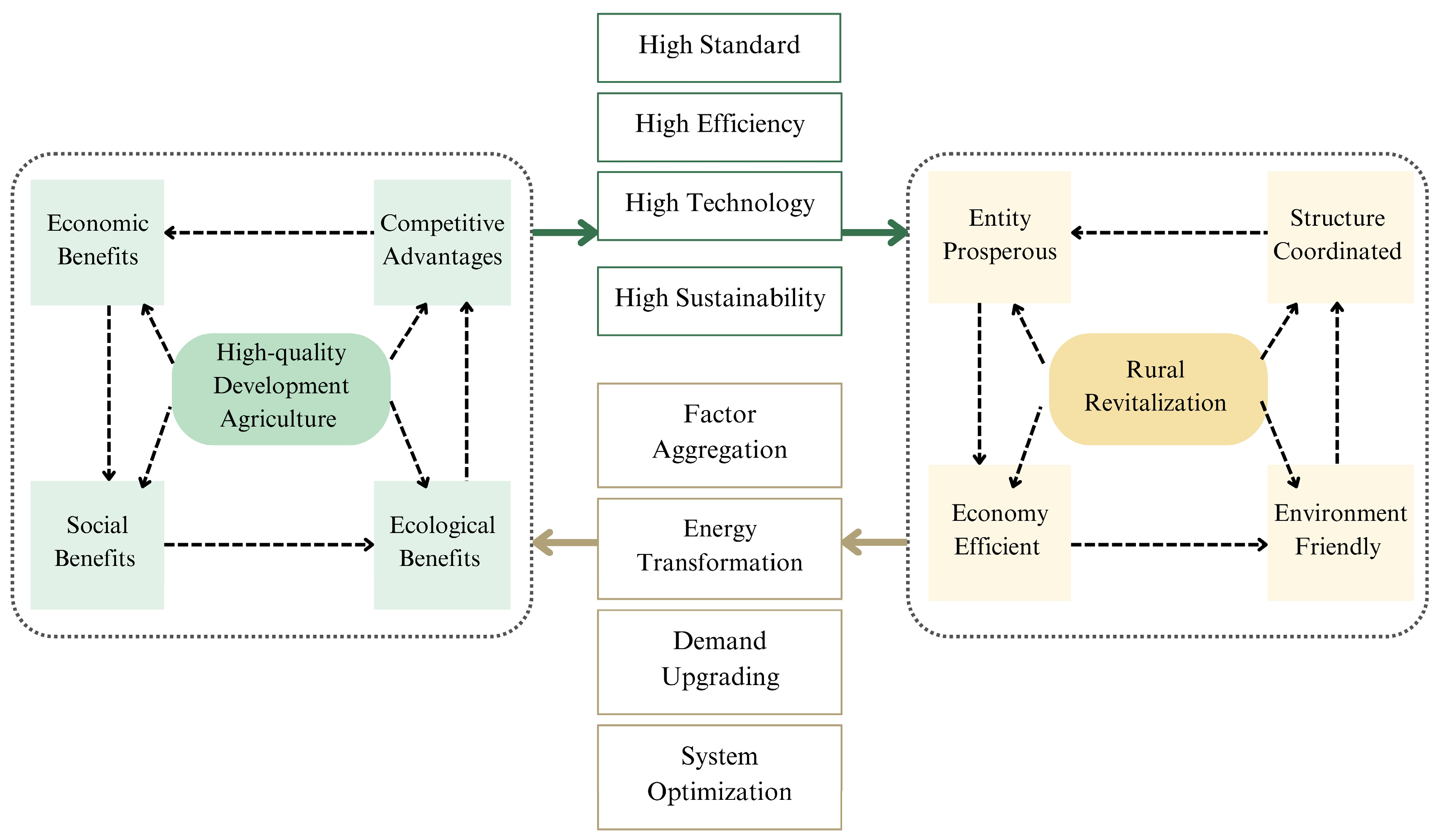
2.3. Mechanism of Mutual Reinforcement between HQAD and Rural Revitalization

The relationship between the rural revitalization system and the HQAD system is characterized by development dynamics and interlinkages. While each has its own focus, both fundamentally construct and form an understanding of multiple functions of agriculture, multiple attributes of farmers, and multiple values of rural areas. They share similar driving forces, endogenous construction subjects, and common resource bases, and both encompass industrial upgrading, ecological sustainability, and income increase in their construction content. Overall, the ultimate goal is to address the ‘three new rural issues’, and to achieve China’s supply side structural reform and modernization of rural agriculture.
The improvement in agricultural modernization is directly linked to industrial prosperity, which is an essential component of rural revitalization. Also, high-quality development places more dimensions, higher requirements, and richer connotations on agriculture. Through high-quality development, agriculture achieves economic, social, ecological benefits, and core competitive advantage optimization. Therefore, it aligns high-standard products, high-efficiency industrial systems, advanced technological means, and energy-saving green sustainable production and operation methods with livable ecology, civilized civilization, effective governance, and prosperous life in rural revitalization, achieving their coordinated advancement.
Also, the realization of rural revitalization can attract various factors to converge in rural areas and agricultural sector. The increasing consumption demand of residents driving the improvement in production efficiency and quality, facilitated by factors acting on the production–supply system in agriculture. The optimization of finance, law, land, and other systems, and the establishment of comprehensive development platforms for rural areas, provide assurance and impetus for the priority of agricultural quality, therefore promoting the HQAD system and its six secondary subsystems.
Based on system theory, this study constructs a ‘combined, function-induced, dual-linkage’ mechanism for the interaction between HQAD and rural revitalization, which is a bidirectional, cyclic dynamic feedback system (see Figure 2). The relationship between high-quality agricultural development and rural revitalization is coordinated and mutually promoted, exhibiting a systematic, complex, multi-dimensional linkage, and bidirectional interaction. The elements within the system restrict and influence each other, showcasing multiple correlations based on functional differences.

3. Methodology

3.1. Improved AHP–Entropy Weight Method

Drawing from existing literature, this study ultimately adopts a combined subjective and objective weighting method, using the analytic hierarchy process (AHP) and an improved entropy method [42] for the index weight determination.

3.1.1. Analytical Hierarchy Process (AHP)

The analytic hierarchy process (AHP) is a multi-objective problem-solving method which is a hybrid of qualitative and quantitative approaches [43]. It uses the decision maker’s experience to measure the relative importance of each goal and reasonably assigns weights to each standard for each solution, using these weights to derive the priority of each solution.
Steps of AHP to obtain subjective weights are as follows:
Step 1: Construct the comparison judgment matrix.
According to the indicator system of high-quality agricultural development and rural revitalization, shown in Table 1 and Table 2, 30 experts in the field of agricultural economics were invited to summarize their opinions. Using the AHP method, from the subsystem level to the criterion level and the indicator level, a weight-scoring matrix R is established by the pairwise comparison of the relative importance of indicators within the same level:
R = r 11 r 12 r 1 i r 21 r 22 r 2 i r j 1 r j 2 r j i   ( w h e r e   i   a n d   j   a r e   p o s i t i v e   i n t e g e r s )
Constructing the judgment matrix using a 1–9 scale method [44] (see Table 2), the importance of each evaluation indicator in the evaluation layer is judged. The maximum eigenvalue λ m a x and the corresponding eigenvector W of the judgment matrix A are calculated using the eigenvalue method, and consistency is tested. Suppose there are n indicators, the judgment matrix is A = ( a i j ) n × n , where a i j indicates the importance of indicator i compared to indicator j . If factor i is compared to j and judged as   A i j , then the judgment of factor j to i is   A j i = 1   A j i . The geometric mean of the scoring matrices from multiple experts is taken to perform an AHP analysis on the resulting summary matrix.
Step 2: Calculate the consistency index (CI).
The judgment matrix requires consistency and transitivity. This study tests the consistency of the eigenvalues and eigenvectors of the judgment matrix to ensure its logical rationality. CI measures the level of deviation of the matrix from complete consistency, and its calculation formula is:
C I = λ m a x n n 1
Step 3: Calculate the consistency ratio (CR).
The consistency test is passed when CR < 0.1, or it indicates logical inconsistencies in the judgment matrix, which need to be appropriately corrected or re-evaluated. The calculation formula is:
C R = C I R I
where RI is the average random consistency index of the same order, and n represents the matrix order (see Table 3).

3.1.2. Improved Entropy Method

The entropy method is an objective weighting method based on the variability of the evaluation indicator data information. To ensure the comparability of results across different years, an improved entropy method [41] with a time variable is used in the indicator-weighting procedure.
Step 1: Data standardization.
Standardize each indicator, where x θ i j is the initial value of province i for indicator j in year θ, and y θ i j is the standardized value of each indicator.
y θ i j = x θ i j x j m i n x j m a x x j m i n ,   Benefit   indicator   x j m a x x θ i j x j m a x x j m i n ,   Cost   indicator  
Step 2: Matrix normalization.
Normalize the standardized matrix and calculate the probability matrix of the indicator values for province i under indicator j in year θ .
P θ i j = y θ i j θ = 1 r i = 1 n y θ i j
Step 3: Calculate the information entropy.
Following the definition, the information entropy of indicator j is:
e j = k θ = 1 r i = 1 n P θ i j ln ( P θ i j )
where k > 0, k = 1 / l n ( r × n ) , and 0 e j 1 .
Step 4: Calculate the weight of each indicator j .
w j = ( 1 e j ) / j = 1 n ( 1 e j )

3.1.3. Combined Weighted Model Based on the AHP and Improved Entropy

Using the combined weighting of the analytic hierarchy process (AHP) and the improved entropy method, the formula for the calculation of the comprehensive weight is:
λ j = θ j W j j = 1 n θ j W j
where λ j is the comprehensive weight of indicator j , n is the number of indicators, θ j is the subjective weight determined by the AHP, and W j is the objective weight obtained through the entropy method.

3.2. Coupling Coordination Degree Model

The coupling coordination evaluation model [45,46] is selected to empirically test whether HQAD and rural revitalization can achieve coordinated development.
Step 1: Obtain the coupling degree of HQAD and rural revitalization.
The formula is as follows:
C = u 1 × u 2 / u 1 + u 2 2 1 2
where   u 1 represents the HQAD evaluation function, and u 2 represents the rural revitalization evaluation function. C represents the coupling degree value, ranging from [0, 1], with higher values indicating better conditions.
Step 2: Compute the coupling coordination degree (CCD) of HQAD and rural revitalization.
The CCD model is constructed as follows:
C C D = C × T
T = α u 1 + β u 2
where C C D is the coupling coordination degree, T is the system’s comprehensive coordination index, and α and β are undetermined coefficients. Considering the status and importance of the two systems, the common practice and expert scoring were referenced to determine the undetermined coefficients for the HQAD and rural revitalization systems, with both α and β set to 0.5. The CCD ranges from [0, 1], with higher values indicating better coupling coordination [47].
To ensure comprehensiveness and clarity, this study adopts the ‘six-division method’ based on the research results of several scholars [48,49,50] to classify the CCD into different intervals. The classifications of CCD are shown in the following Table 4.

3.3. Kernel Density Estimation

The kernel density estimation (KDE) method is commonly used to depict the evolution trajectory of the CCD between HQAD and rural revitalization, referencing existing research [51,52,53]. The calculation formula is:
f x = 1 N h i = 1 N K D i D ¯ h
where f x is the probability density function of the coupling coordination degree, N is the size of the sample, h is the bandwidth, K is the KDE function, D i is the CCD, and D ¯ is the average value of the CCD. The Gaussian kernel density function is mainly used for estimation:
K D ¯   = 1 2 π exp D 2 ¯   2

3.4. Dagum Gini Coefficient

The Dagum Gini coefficient method is used to the reveal regional disparities and sources of the CCD between HQAD and rural revitalization. The higher the value, the greater the regional disparities, and vice versa. The detailed calculation process is based on existing research [54,55].
Step 1: Calculate the overall Gini coefficient G .
G = j = 1 k h = 1 k i = 1 n j r = 1 n h y j i y h r   2 n 2 μ
where y ji and y hr are the CCDs of any province in region j (h); respectively, μ is the mean of CCD, n (equal to 30) is the number of provinces, k (equal to 4) is the number of regions nationwide, and n j and n h are the numbers of provinces in regions j (h), respectively. G is the aggregate Gini coefficient,   G w is the contribution values of intra-regional differences, G nb is the inter-regional differences [56], and G t is the hyper variable density, which satisfies G =   G w + G nb +   G t .
Step 2: Calculate the contribution value of intra-regional differences G w .
G j j = i = 1 n j r = 1 n j y j i y j r 2 n j 2 y j ¯
G w = j = 1 k G j j p j s j
where p j = n j / n , s j = n j y j ¯ / n y ¯ , G j j represents the intra-regional Gini coefficient, n j is the number of provinces in region j , y j ¯ is the average CCD of region j , and y j i and y j r are the CCD of provinces i and r within region j .
Step 3: Calculate the contribution value of the inter-regional differences.
G j h i = 1 n j r = 1 n h y j i y h r n j n h Y j ¯ + Y h ¯
G n b = j = 2 k h = 1 j 1 G j h p j s h + p h s j D j h
D j h = d j h p j h d j h + p j h
d j h = 0 d F j ( y ) 0 y y x d F h ( x )
p j h = 0 d F h   ( y ) 0 y y x d F j ( y )
where p h = n h / n , s h = n h y h ¯ / n y ¯ , G j h represents the inter-regional Gini coefficient, y j ¯ and y h ¯ are the average CCDs of the regions j(h), D j i is the relative influence of the CCDs between regions j and h , d j h is the difference in CCDs, and p j h is the hypervariable first-order distance. F j and F h are the cumulative density distribution functions of regions j and h , respectively.
Step 4: Calculate the contribution value of hyper variable density.
G t = j = 2 k h = 1 j 1 G j h p j s h + p h s j ( 1 D j h )

3.5. Convergence Model

A convergence model is employed to analyze the convergence of the CCD between HQAD and rural revitalization. The commonly used convergence models include σ convergence [57] and β convergence [58,59].

3.5.1. σ Convergence Method

σ convergence measures the regional disparity using the standard deviation and coefficient of variation of the CCD, reflecting the pattern of intra-regional differences. The formula is as follows:
σ = i = 1 n j ( D i j D ¯ j ) 2 / n j / D ¯ j
where D i j represents the CCD of province i in region j , D ¯ j represents the mean CCD of region j , and n j represents the number of provinces in region j .

3.5.2. Spatial β Convergence Method

Building upon the traditional β convergence method, spatial econometric models are introduced, which primarily include three types: spatial Durbin model (SDM), spatial error model (SEM), and spatial autoregressive model (SAR). Additionally, the inverse of the square of the geographical distance is mainly used as the spatial weight matrix. If β < 0 and is significant, it indicates a convergence trend in CCD; otherwise, it suggests the existence of a diffusion phenomenon. The specific model formulas are:
SDM:
ln D i ,   t + 1 D i , t = α + β ln D i , t + θ j n ω i j ln D i , t + ρ j n ω i j ln D i , t + 1 D i , t + u i + υ t + ε i t
SEM:
ln D i ,   t + 1 D i , t = α + β ln D i , t + θ j n ω i j ln D i , t + u i + υ t + ε i t
SAR:
ln D i ,   t + 1 D i , t = α + β ln D i , t + ρ j n ω i j ln D i , t + 1 D i , t + u i + υ t + ε i t
where α is the constant term, β is the spatial regression coefficient, θ is the spatial error coefficient, and ρ is the spatial lag coefficient, reflecting the influence of the CCD’s development level and growth rate in neighboring regions on the local region’s coupling coordination development level. ω i j is the spatial weight matrix, u i represents regional effects, v t represents time effects, and ε i t is the random disturbance term.

4. Spatiotemporal Evolutionary Characteristics of CCD

4.1. Temporal Evolution Characteristics of CCD

By inputting the evaluation results of HQAD and rural revitalization of provinces and municipalities into coupling coordination degree models, the aggregate results exhibit the characteristics of a ‘high coupling degree, low comprehensive development level, and low coupling coordination degree’. As shown in Table 5, from 2010 to 2020, the national coupling degree remained above 0.99, indicating a favorable level of quality coupling. The CCD shows a steady growing trend, although the classification type remains relatively low, persistently in a “barely coordinated” group, far from achieving favorable coordination. Specifically, 2012 and 2016 marked the lowest and highest points within this period, with the coordination degree fluctuating around 0.58 from 2013 to 2019, and a slight decline observed in 2020.

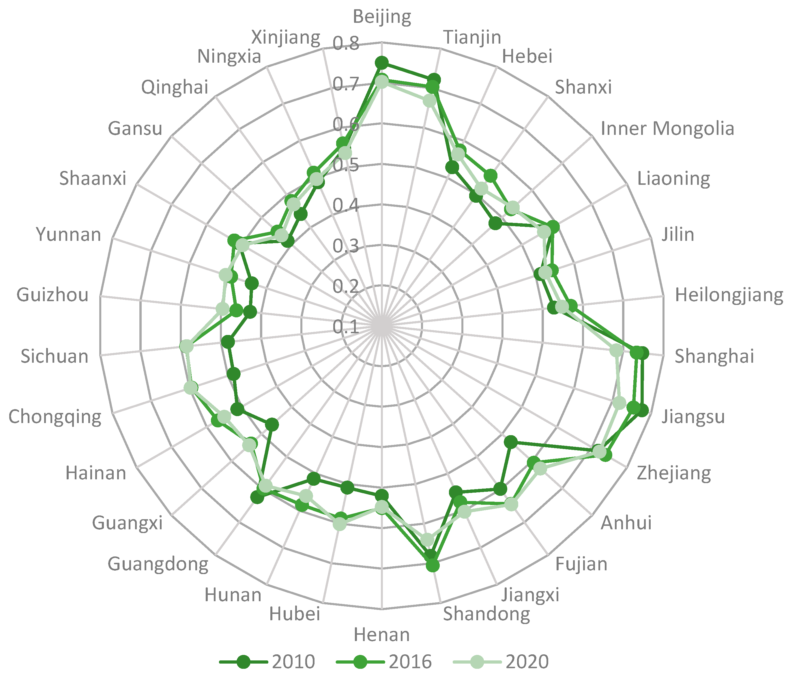
4.2. Spatial Evolutionary Characteristics of CCD

4.2.1. Evolutionary Trends of CCD

Figure 3 reports the dynamic evolution trends of the CCD of HQAD and rural revitalization systems in provinces and municipalities across China in 2010, 2016, and 2020.
The overall results indicate a stable upward trend in CCD across the regions, with a spatial distribution pattern of ‘high in the east and low in the west’. Specifically, in 2010, the CCD in most provinces fluctuated within the range of [0.4, 0.75], followed by a significant increase, reaching the highest level in 2016; and followed by a slight decline observed in 2020, fluctuating within the range of [0.43, 0.73]. In 2010, the CCD ranking of the four major regions was as follows: east (0.6827) > northeast (0.5431) > central (0.5201) > west (0.4738). By 2020, the ranking from highest to lowest was as follows: east (0.6590) > central (0.5764) > northeast (0.5456) > west (0.5203).

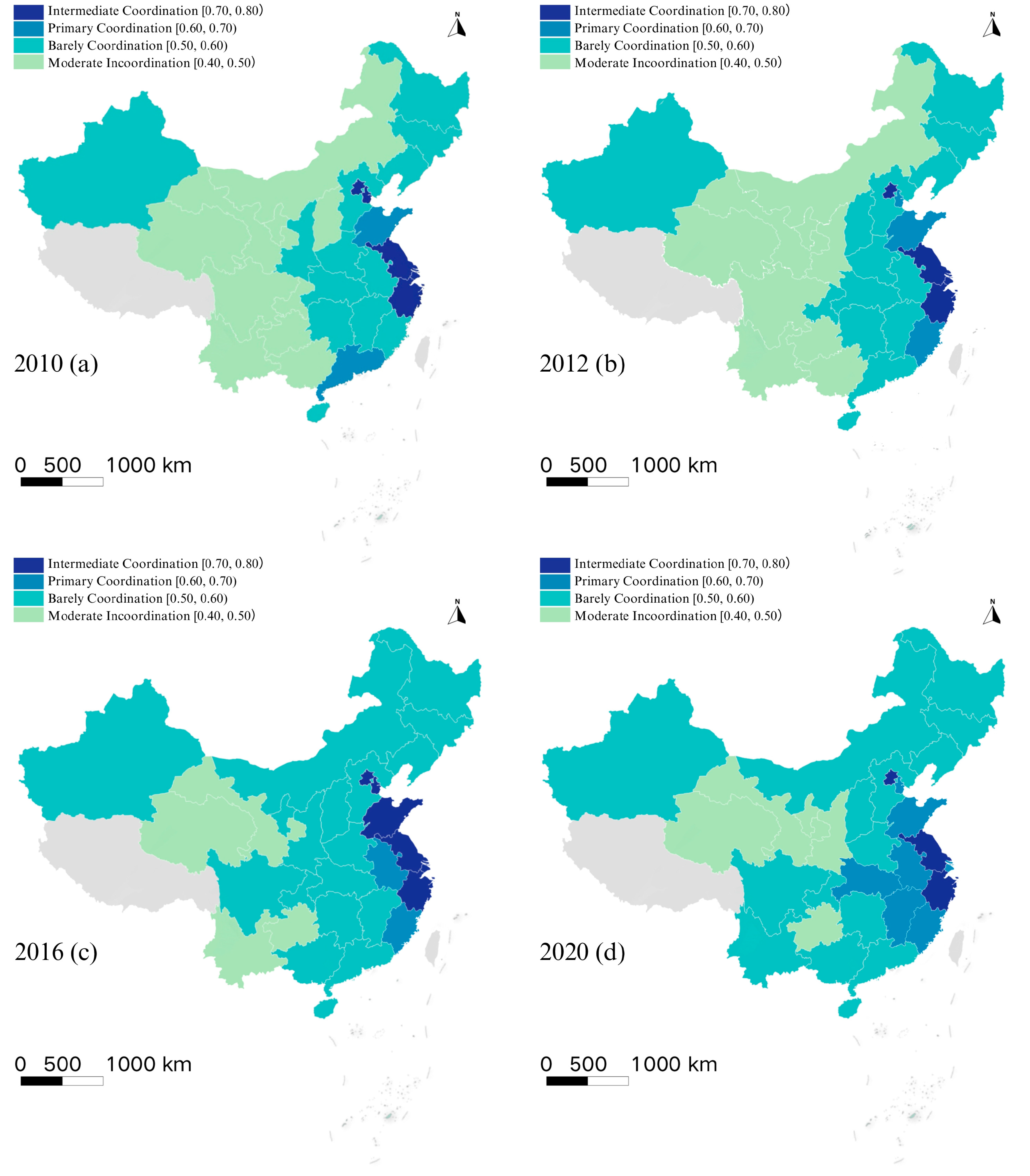
4.2.2. Spatial Differentiation of CCD

According to the classification in Figure 4, during the sample period, no breakthroughs were made in achieving the optimal category of quality coordination. Around four and six provinces located in the current highest level of intermediate coordination group; the number of provinces in the primary coordination group increased annually, from two in 2010 to seven in 2020, while the number of provinces in lower coordination groups continued to decrease.
The overall change in CCD in 2012 compared to 2010 was not significant. A marked improvement was observed since 2016, with more than 83.3% of provinces entering the coordination stage of HQAD and rural revitalization. Specifically, only four provinces have been in a group of moderate incoordination (2016), almost halving the number from nine (2010). The number of provinces categorized as “barely coordinated” increased from 13 in 2010 to 18 in 2016, with a slight decrease to 15 in 2020. Some western provinces remain in a low-value structure or unbalanced development state regarding agricultural development and rural reformation, but the overall CCD is continuously improving. In brief, the CCD of each province shows an increasing trend year by year, with a tendency moving towards higher stages, and there exists a spatial distribution characteristic of ‘high in the east and low in the west’.

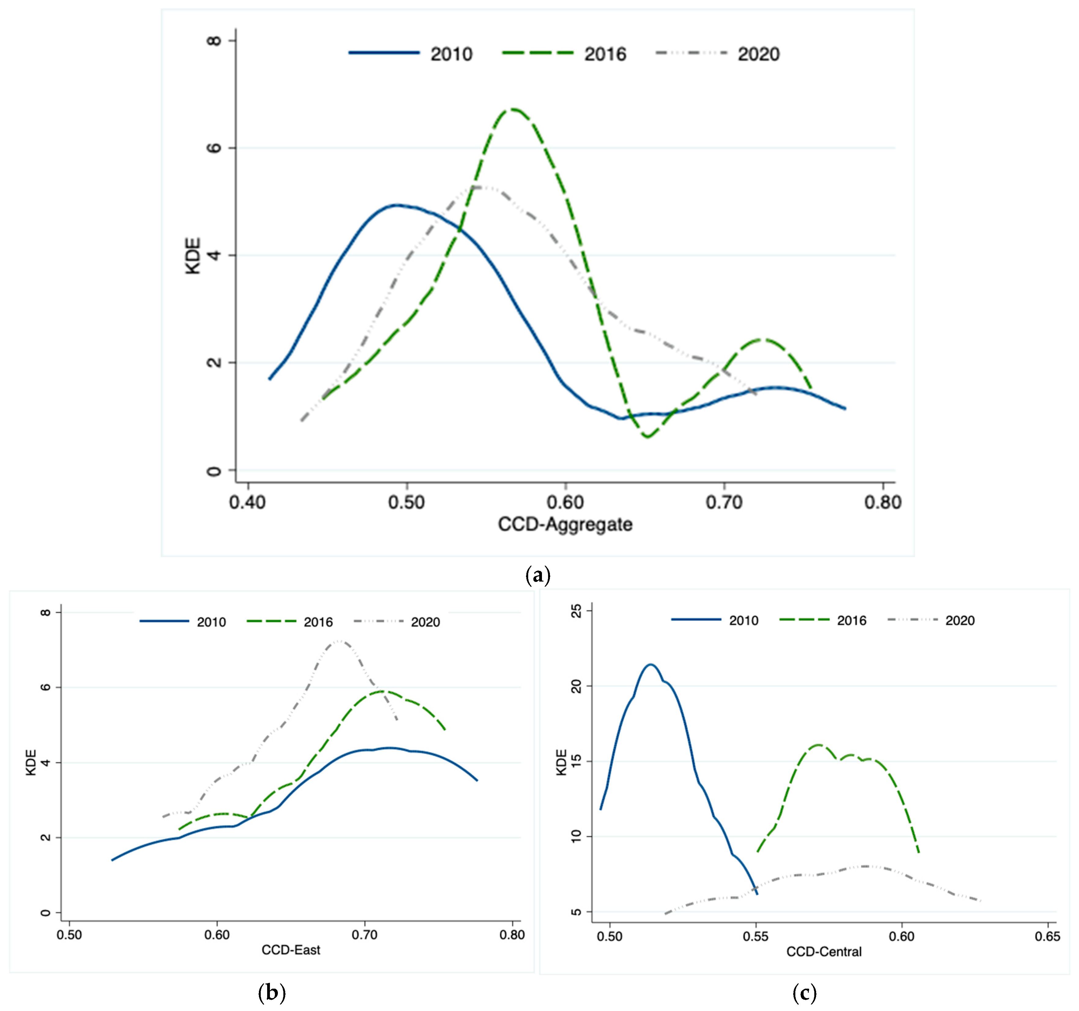
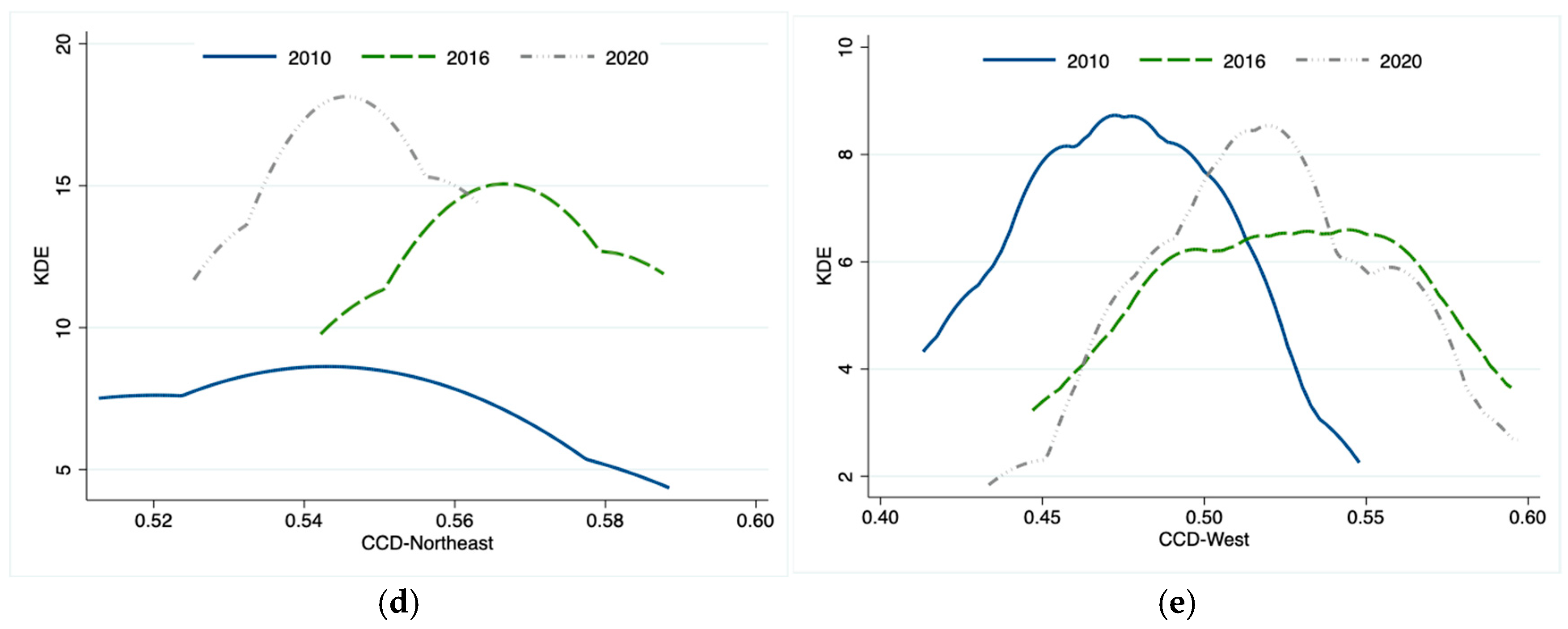
5. Kernel Density Analysis of CCD

Figure 5 depicts the distribution position, shape, extensibility, and polarization of the kernel density estimation (KDE) curves across the nation and the four major regions, further analyzing the dynamic evolution trajectory of the CCD. The analysis primarily presents the changes in the KDE of the CCD between two systems in 2010, 2016, and 2020.
At the national level, the KDE curve displays the evolutionary characteristics of ‘gradually shifting to the right with slight retraction, peak values first increasing then decreasing, narrowing the width, and diminishing the tail phenomena’. The curve shows that although there were short-term regressions, the overall trend towards higher stages of CCD remains unchanged; the peak values climb first and then drop, with the bandwidth slightly narrowing. This indicates the presence of aggregation phenomena across regions, reducing regional disparities and showing a positive adjustment towards favorable coordination. In 2010 and 2016, the KDE curves displayed varying degrees of ‘bimodal’ patterns, then successfully transformed into a ‘unimodal’ pattern in 2020 with diminishing tail phenomena, which indicates that polarization and strong core phenomena among regions are gradually disappearing, and the overall trend is moving towards balanced development.
At the regional level, the KDE curves in the eastern and northeastern regions both show the evolutionary characteristics of ‘gradually shifting to the right with significant retraction’, with CCDs fluctuating but still improving, and the overall trend showing good coordination from the perspectives of peak values, bandwidth, peak numbers, and tail situations. The northeastern region shows a process of ‘diffusion–aggregation’, with regional disparities first widening and then narrowing; the curves are essentially uncrossed, indicating small differences in CCDs, with no regions lagging. The central and western regions have a similar distribution, shape, and extensibility characteristics, with the CCDs gradually increasing and concentrating, mainly showing a ‘unimodal’ pattern with insignificant polarization. However, in 2020, the central region saw rapid expansion in width and significant tail phenomena, indicating that the CCD disparity has increased, with strong core characteristic regions emerging.

6. Regional Disparities and Sources of CCD

The Dagum Gini coefficient is used to decompose the CCD in China and the four regions in detail, revealing the spatial disparities and the sources (Table 6 and Table 7).

6.1. Aggregate Regional Disparities and Intra-Region Disparities of CCD

As shown in Table 7, the aggregate Gini coefficient fluctuates within the range of [0.07, 0.09], showing a declining trend, with a decrease of 28%, except for slight rebounds in 2011 and 2018, indicating that regional disparities in CCD are gradually narrowing nationwide.
Referring to the four major regions in China (see Table 6), the average Gini coefficient during the sample period ranks as follows: east (0.507) > west (0.469) > central (0.0232) > northeast (0.0188). Among them, the Gini coefficient in the eastern region fluctuated within the range of [0.04, 0.06], showing a continuous decline from 2010 to 2017, followed by a slight rebound after 2018. The western and northeastern regions show similar trends in the Gini coefficient, but with significant differences in values, fluctuating and declining within the ranges of [0.04, 0.05] and [0.01, 0.03], respectively, with frequent but small fluctuations. For the central region, the Gini coefficient shows a ‘W’ shaped fluctuation, with an increasing trend in regional disparities. Overall, compared to the initial values in 2010, the aggregate disparities in CCD, as well as in eastern, and northeastern regions, show a declining trend, with little change in the western region and an increase in the central region.

6.2. Inter-Regional Disparities of CCD

As shown in Table 6, the ranking of the average inter-regional disparities in CCD from largest to smallest is: east–west (0.1473) > east–central (0.1017) > east–northeast (0.0976) > west–northeast (0.0576) > central–west (0.0542) > central–northeast (0.0287). Overall, the disparity in CCD values between the eastern region and other regions is higher than the disparity among non-eastern regions. The non-equilibrium between the western region and other regions is particularly prominent. Among them, the Gini coefficients between the east–west regions, east–central regions, and west–northeast regions all show a stable downward trend, while the results between the east–northeast regions fluctuates frequently, with a small overall decline. However, the disparities in CCD between the central–western regions and central–northeastern regions show an expanding trend, with inter-regional non-equilibrium issues needing urgent resolution.

6.3. Sources of Regional Disparities and Contributions of CCD

As shown in Table 7, from 2010 to 2020, the contribution rates of the aggregate regional disparities rank as follows: inter-regional disparities > intra-regional disparities > hyper variance density. The contribution rates of inter-regional disparities fluctuate within the range of 75.77–84.58%, showing a slight decline, while the contribution rates of intra-regional disparities and hyper variance density show an increasing trend. Overall, the fluctuations are small and relatively stable, with inter-regional disparities consistently dominating, indicating that the inter-regional unbalance is still significant.

7. Convergence Analysis of CCD

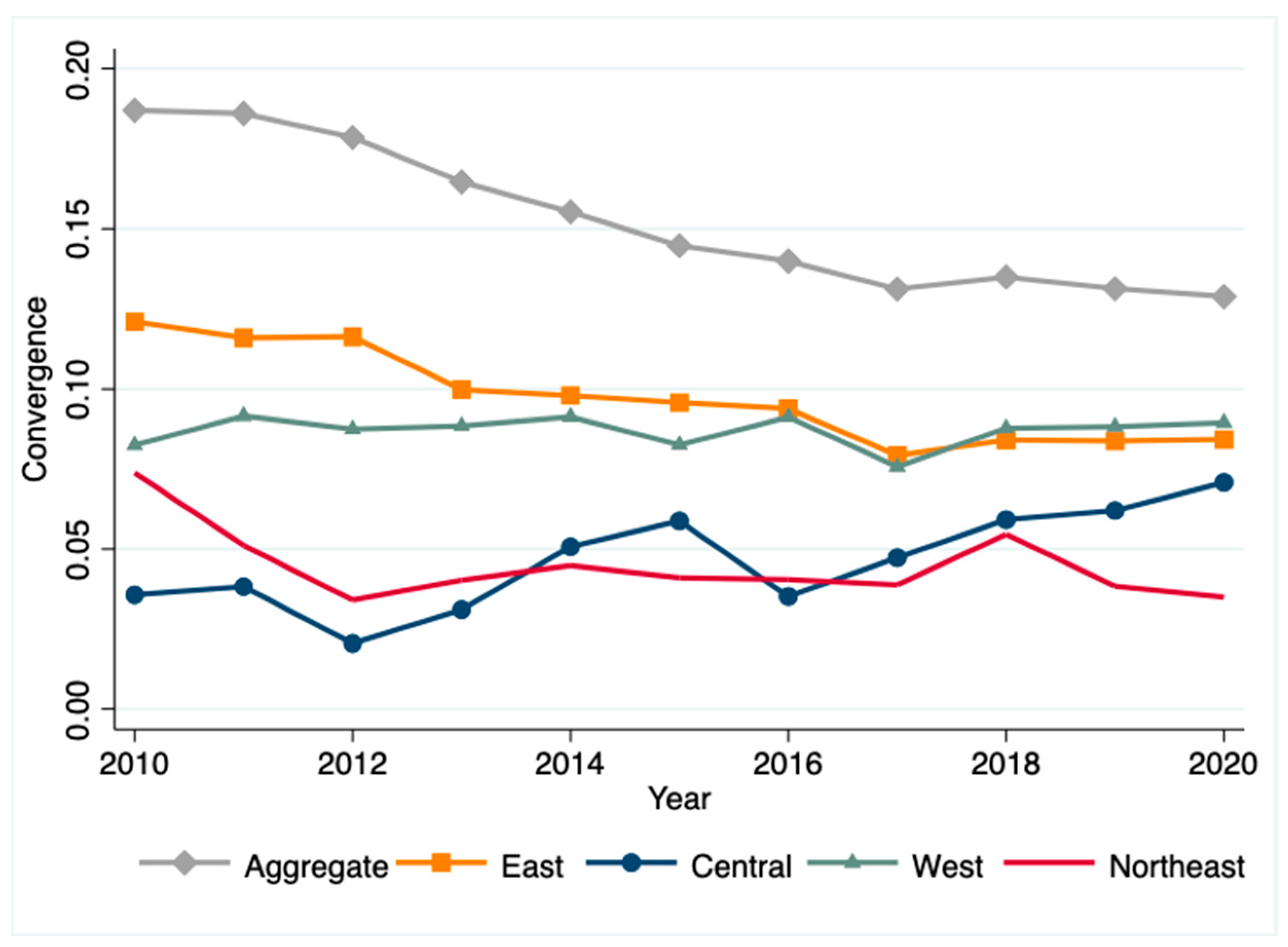
7.1. σ Convergence Test

Using the σ convergence method, the convergence characteristics of the CCD in China and four regions from 2010 to 2020 are analyzed. As shown in Figure 6, the convergence coefficient in China shows a clear convergence trend. Specifically, the curve in the eastern region is similar in shape to that of in China; while the curves in the western and northeastern regions are similar, with small fluctuations and a slight downward trend. The central region’s convergence coefficient shows a ‘W’-shaped fluctuation. Overall, except for the central region, the CCD in other regions shows a certain degree of convergence.

7.2. Spatial β Convergence Test

The spatial β convergence method is employed to explore the convergence effects of the CCD in China and four regions, with the Hausman, LM, LR, and Wald tests used to select appropriate spatial econometric models to improve the accuracy of the research conclusions. The spatial fixed SDM model is selected for China, Central, and Western regions, while the OLS model is used for the eastern and northeastern regions due to the failure to pass the LM test.
As shown in Table 8, the spatial regression coefficients β are significantly negative at the 1% level, indicating the presence of β convergence, where regions with lower CCDs catch up with higher-level regions over time, ultimately achieving steady-state equilibrium. Based on the absolute values of the convergence coefficients, the central region has the fastest convergence speed, followed by the western and northeastern regions, with the northeast having the slowest. The error coefficient θ and lag coefficient ρ in the China, Central, and Western regions are significantly positive at the 1% level, indicating positive spatial correlation, which means that changes in CCDs are positively influenced by other regions, and external spillover effects effectively promote the improvement in CCD in the local region.

8. Conclusions and Recommendations

By employing the panel data from China and 30 provinces from 2010 to 2020, an analysis was conducted on the measurement and CCD evaluation between HQAD and rural revitalization. The results show the following: (1) The CCDs in regions generally shows a stable upward trend, with a spatial distribution pattern of ‘higher in the east and lower in the west’. The coordination type also has the potential to rise to a higher group, but there is still a significant gap to reach optimal coordination. The overall trend in the KDE curve indicates a well-balanced development, with short-term adjustments and fluctuations. (2) The aggregate regional disparity in the Gini coefficient continues to decline, but regional disparities in the central and western regions warrant attention. The gap between the eastern region and other regions is relatively significant, with regional disparities mainly originating from inter-regional differences. (3) The results of σ convergence and spatial β convergence reflect that the CCD between two systems exhibits a certain degree of convergence. Regional development imbalances resulting from variations in economic and social development foundations and factor endowments inevitably affect the sustainable development of rural areas and the agricultural sector under the broader socio-economic system [60].
According to the above results, the following recommendations are provided: (1) Comprehensively constructing a high-quality development framework for agriculture and rural areas will promote the implementation of rural revitalization. Macro-coordination from the perspective of ‘big industry’, and building a rural industrial development system of ‘agriculture +’ insisting agriculture will be at the core of this framework. The government should always pay attention to the key role and interlinked mechanism of HQAD in achieving comprehensive rural revitalization. (2) Addressing the issues of unbalanced development and narrowing the regional gaps should be the focus of the government’s economic development efforts. Through the radiating and leading role of the dominant regions, the coordinated development of the neighboring regions will be driven and the overall level of regional development will be enhanced. (3) Adopting differentiated development strategies according to local conditions and building a spatial layout structure will provide complementary advantages. Fully utilizing the spatial diffusion effect, the efficient and orderly flow of resource elements can be guided, the resource endowments of the region can be tapped into, and collaboration with neighboring regions will yield complementary advantages and strengthen inter-regional cooperation.

Author Contributions

Conceptualization, Y.W.; methodology, Y.W. and M.H.S.; software, Y.W. and Y.L.; validation, Y.W. and Y.L.; formal analysis, Y.W. and M.H.S.; data curation, Y.W. and Y.L.; writing—original draft preparation, Y.W.; writing—review and editing, Y.W. and M.H.S.; visualization, Y.W. and Y.L.; supervision, M.H.S.; funding acquisition, Y.W. All authors have read and agreed to the published version of the manuscript.

Funding

This research was funded by the Scientific Research Project of Hunan Provincial Department of Education in China, grant number: 23B0281.

Data Availability Statement

The original report data come from the China Rural Statistical Yearbook, China Agricultural Yearbook, China Rural Management Statistical Annual Report, China Agricultural Machinery Industry Yearbook, China Leisure Agriculture Yearbook. All the aforementioned data were purchased by Central South University of Forestry and Technology, where the authors work or study.

Conflicts of Interest

The authors declare no conflicts of interest.

References

  1. Matlovič, R.; Matlovičová, K. Polycrisis in the Anthropocene as a Key Research Agenda for Geography: Ontological Delineation and the Shift to a Postdisciplinary Approach. Folia Geogr. 2024, 66, 5–33. [Google Scholar]
  2. Onitsuka, K.; Hoshino, S. Inter-community Networks of Rural Leaders and Key People: Case Study on a Rural Revitalization Program in Kyoto Prefecture, Japan. J. Rural Stud. 2018, 61, 123–136. [Google Scholar] [CrossRef]
  3. Bai, X.; Shi, P.; Liu, Y. Society: Realizing China’s Urban Dream. Nature 2014, 509, 158–160. [Google Scholar] [CrossRef]
  4. Rigg, J.; Ritchie, M. Production, Consumption, and Imagination in Rural Thailand. J. Rural Stud. 2002, 18, 359–371. [Google Scholar] [CrossRef]
  5. Zhang, J.; Zeng, Z.; Li, G. Theoretical Interpretation and Logical Mechanism of High-Quality Agricultural Economic Development in the New Era. Agric. Econ. 2023, 4, 3–5. [Google Scholar]
  6. Li, K.; Yang, N.; Feng, L. Problems and Development Strategies in the Process of High-Quality Agricultural Development in China. Agric. Econ. 2023, 3, 32–33. [Google Scholar]
  7. Xin, L.; An, X. Construction and Empirical Analysis of Agricultural High-quality Development Evaluation System in China. Econ. Rev. 2019, 5, 109–118. [Google Scholar]
  8. Feng, L.; Chen, Z.; Ma, Y. Research on the Impact of Land Transfer Policy on High-Quality Agricultural Development. Stat. Decis. 2022, 19, 76–79. [Google Scholar]
  9. Wang, H.; Tang, Y. Spatiotemporal Distribution and Influencing Factors of Coupling Coordination between Digital Village and Green and High-Quality Agricultural Development—Evidence from China. Sustainability 2023, 15, 8079. [Google Scholar] [CrossRef]
  10. Wang, Y.; Xie, L.; Zhang, Y.; Wang, C.; Yu, K. Does FDI Promote or Inhibit the High-Quality Development of Agriculture in China? An Agricultural GTFP Perspective. Sustainability 2019, 11, 4620. [Google Scholar] [CrossRef]
  11. Cui, X.C.; Cai, T.; Deng, W.; Zheng, R.; Jiang, Y.; Bao, H. Indicators for Evaluating High-Quality Agricultural Development: Empirical Study from Yangtze River Economic Belt, China. Soc. Indic Res. 2022, 164, 1101–1127. [Google Scholar] [CrossRef]
  12. Ye, X. Enhancing the Inclusiveness of Rural Revitalization to Promote Common Prosperity among Farmers and Rural Areas. China Rural Econ. 2022, 2, 2–14. [Google Scholar]
  13. Chen, M.; Zhou, Y.; Huang, X.; Ye, C. The Integration of New-Type Urbanization and Rural Revitalization Strategies in China: Origin, Reality, and Future Trends. Land 2021, 10, 207. [Google Scholar] [CrossRef]
  14. Chen, J.; Shi, H.; Lin, Y. Research on the Evaluation System and Method of Rural Revitalization Level: A Case Study of Six Provinces in East China. East China Econ. Manag. 2021, 35, 91–99. [Google Scholar]
  15. Mao, J.; Wang, L. Construction of the Evaluation Index System of Rural Revitalization: An Empirical Study Based on the Provincial Level. Stat. Decis. 2020, 19, 181–184. [Google Scholar]
  16. Zhang, T.; Li, M.; Xu, Y. Construction and Empirical Research on the Evaluation Index System of Rural Revitalization. Manag. World 2018, 34, 99–105. [Google Scholar]
  17. Zha, Q.; Liu, Z.; Song, Z.; Wang, J. A Study on Dynamic Evolution, Regional Differences, and Convergence of High-Quality Economic Development in Urban Agglomerations: A Case Study of Three Major Urban Agglomerations in the Yangtze River Economic Belt. Front. Environ. Sci. 2022, 10, 1012304. [Google Scholar] [CrossRef]
  18. Lu, F.; Pang, Z.; Deng, G. Measurement of Regional Differences and Formation Mechanisms of Rural Revitalization Development in China. Explor. Econ. Issues 2022, 4, 19–36. [Google Scholar]
  19. Haiyirete, X.; Xu, Q.; Wang, J.; Liu, X.; Zeng, K. Comprehensive Evaluation of the Development Level of China’s Characteristic Towns under the Perspective of an Urban–Rural Integration Development Strategy. Land 2024, 13, 1069. [Google Scholar] [CrossRef]
  20. Chen, D.; Hu, W. Temporal and Spatial Effects of Heavy Metal-Contaminated Cultivated Land Treatment on Agricultural Development Resilience. Land 2023, 12, 945. [Google Scholar] [CrossRef]
  21. Sun, P.; Ge, D.; Yuan, Z.; Lu, Y. Rural Revitalization Mechanism Based on Spatial Governance in China: A Perspective on Development Rights. Habitat Int. 2024, 147, 103068. [Google Scholar] [CrossRef]
  22. Diedrich, A.; Benham, C.; Pandihau, L.; Sheaves, M. Social Capital Plays a Central Role in Transitions to Sportfishing Tourism in Small-Scale Fishing Communities in Papua New Guinea. Ambio 2019, 48, 385–396. [Google Scholar] [CrossRef]
  23. Jing, Z.; Yu, Y.; Wang, Y.; Su, X.; Qiu, X.; Yang, X.; Xu, Y. Study on the Mechanism of Livelihood Behavior Decision of Rural Residents in Ethnic Tourism Villages in Western Sichuan. Ecol. Indic. 2024, 166, 112250. [Google Scholar] [CrossRef]
  24. Jia, X. Digital Economy Factor Allocation and Sustainable Agricultural Development: The Perspective of Labor and Capital Misallocation. Sustainability 2023, 15, 4418. [Google Scholar] [CrossRef]
  25. Dong, Z.; Zhao, C. Path Selection for High-Quality Agricultural and Rural Development under the Background of Rural Revitalization. J. Party Sch. Cent. Comm. CPC 2022, 26, 80–88. [Google Scholar]
  26. Yang, X.; Liang, Y. The Logical Foundation, Restrictive Factors, and Institutional Supply of High-Quality Industrial Development from the Perspective of Rural Revitalization. Hubei Soc. Sci. 2023, 4, 87–93. [Google Scholar]
  27. Xie, Y.; Qi, C. Mechanism and Countermeasures for the Linkage between High-Quality Agricultural Development and Rural Revitalization. Zhongzhou Acad. J. 2020, 2, 33–37. [Google Scholar]
  28. Yang, S.; Jiang, L. Study on the Spatial and Temporal Effects of High-Quality Agricultural Development on Rural Revitalization. Stat. Decis. 2023, 39, 116–120. [Google Scholar]
  29. Meng, F.; Ding, S. Research on the Coupling and Coordination Relationship between Rural Revitalization and High-Quality Agricultural Development. Stat. Decis. 2024, 40, 79–83. [Google Scholar]
  30. Qi, C.; Liu, X.; Wu, W.; Yuan, J. Spatial Correlation and Coupling Coordination Evaluation between High-Quality Development and Rural Revitalization in the Yellow River Basin. Stat. Decis. 2024, 40, 124–128. [Google Scholar]
  31. Lu, P.; Yu, S. Research on the Coordinated Development Trend of New Urbanization and Rural Revitalization in China. Econ. Perspect. 2021, 11, 76–82. [Google Scholar]
  32. Wei, C.; Zhang, Z.; Ye, S.; Hong, M.; Wang, W. Spatial-Temporal Divergence and Driving Mechanisms of Urban-Rural Sustainable Development: An Empirical Study Based on Provincial Panel Data in China. Land 2021, 10, 1027. [Google Scholar] [CrossRef]
  33. Ding, C.; Yang, F.; Guo, Q. Research on the Coupling and Coordinated Development of New Industrialization, New Urbanization, and Rural Revitalization. Stat. Decis. 2020, 36, 71–75. [Google Scholar]
  34. Du, M.; Huang, Y.; Dong, H.; Zhou, X.; Wang, Y. The Measurement, Sources of Variation, and Factors Influencing the Coupled and Coordinated Development of Rural Revitalization and Digital Economy in China. PLoS ONE 2022, 17, e0277910. [Google Scholar] [CrossRef]
  35. Wu, R. Measurement Evolution and Spatial Effect of Coupling Coordination between Tourism High-Quality Development and Rural Revitalization. Ph.D. Thesis, Jiangxi University of Finance and Economics, Nanchang, China, 2022. [Google Scholar]
  36. Lu, Y. Issues of Agricultural and Rural Modernization in Rural Revitalization. J. China Agric. Univ. (Soc. Sci. Ed.) 2018, 3, 48–56. [Google Scholar]
  37. Yang, J.; Yang, R.; Chen, M.H.; Su, C.H.J.; Zhi, Y.; Xi, J. Effects of Rural Revitalization on Rural Tourism. J. Hosp. Tour. Manag. 2021, 47, 35–45. [Google Scholar] [CrossRef]
  38. Yang, X.; Li, W.; Zhang, P.; Chen, H.; Lai, M.; Zhao, S. The Dynamics and Driving Mechanisms of Rural Revitalization in Western China. Agriculture 2023, 13, 1448. [Google Scholar] [CrossRef]
  39. Rao, Y.; Zou, Y.; Yi, C.; Luo, F.; Song, Y.; Wu, P. Optimization of Rural Settlements Based on Rural Revitalization Elements and Rural Residents’ Social Mobility: A Case Study of a Township in Western China. Habitat Int. 2023, 137, 102851. [Google Scholar] [CrossRef]
  40. Ma, M.; Tang, J.; Dombrosky, J.M. Coupling Relationship of Tourism Urbanization and Rural Revitalization: A Case Study of Zhangjiajie, China. Asia Pac. J. Tour. Res. 2022, 27, 673–691. [Google Scholar] [CrossRef]
  41. Wang, Y.; Kuang, Y. Evaluation, Regional Disparities, and Driving Mechanisms of High-Quality Agricultural Development in China. Sustainability 2023, 15, 6328. [Google Scholar] [CrossRef]
  42. Xie, C.; Dong, D.; Hua, S.; Xin, X.; Chen, Y. Safety Evaluation of Smart Grid Based on AHP-Entropy Method. Syst. Eng. Procedia 2012, 4, 203–209. [Google Scholar]
  43. Bai, L.; Wang, H.; Huang, N.; Du, Q.; Huang, Y. An Environmental Management Maturity Model of Construction Programs Using the AHP-Entropy Approach. Int. J. Environ. Res. Public Health 2018, 15, 1317. [Google Scholar] [CrossRef]
  44. Wu, G.; Duan, K.; Zuo, J.; Zhao, X.; Tang, D. Integrated Sustainability Assessment of Public Rental Housing Community Based on a Hybrid Method of AHP-Entropy Weight and Cloud Model. Sustainability 2017, 9, 603. [Google Scholar] [CrossRef]
  45. Yang, C.; Zeng, W.; Yang, X. Coupling Coordination Evaluation and Sustainable Development Pattern of Geo-Ecological Environment and Urbanization in Chongqing Municipality, China. Sustain. Cities Soc. 2020, 61, 102271. [Google Scholar] [CrossRef]
  46. Shi, T.; Yang, S.; Zhang, W.; Zhou, Q. Coupling Coordination Degree Measurement and Spatiotemporal Heterogeneity between Economic Development and Ecological Environment—Empirical Evidence from Tropical and Subtropical Regions of China. J. Clean. Prod. 2020, 244, 118739. [Google Scholar] [CrossRef]
  47. Yang, H.; Xu, X. Coupling and Coordination Analysis of Digital Economy and Green Agricultural Development: Evidence from Major Grain Producing Areas in China. Sustainability 2024, 16, 4533. [Google Scholar] [CrossRef]
  48. Zhang, Y.; Khan, S.U.; Swallow, B.; Liu, W.; Zhao, M. Coupling Coordination Analysis of China’s Water Resources Utilization Efficiency and Economic Development Level. J. Clean. Prod. 2022, 373, 133874. [Google Scholar] [CrossRef]
  49. Deng, M.; Chen, J.; Tao, F.; Zhu, J.; Wang, M. On the Coupling and Coordination Development between Environment and Economy: A Case Study in the Yangtze River Delta of China. Int. J. Environ. Res. Public Health 2022, 19, 586. [Google Scholar] [CrossRef]
  50. Liu, J.; Ma, Y. Research on the Coupled Growth Evolution and Driving Mechanisms of Tourism Flow and Destination Supply and Demand Based on Phylogenetics and System Theory: A Case Study of Xi’an City. Geogr. Res. 2017, 36, 1583–1600. [Google Scholar]
  51. Zhong, S.; Shao, J. Research on the Distribution Dynamics, Spatial Differences, and Convergence of Innovation Development in the Yellow River Basin. J. Quant. Tech. Econ. 2022, 39, 25–46. [Google Scholar]
  52. Senga Kiesse, T.; Corson, M.S. The Utility of Less-Common Statistical Methods for Analyzing Agricultural Systems: Focus on Kernel Density Estimation, Copula Modeling, and Extreme Value Theory. Behaviormetrika 2023, 50, 491–508. [Google Scholar] [CrossRef]
  53. Yang, Y.D.; Sun, C.Z. Assessment of Land–Sea Coordination in the Bohai Sea Ring Area and Spatial–Temporal Differences. Resour. Sci. 2014, 36, 691–701. [Google Scholar]
  54. Zhou, R.; Jin, J.; Cui, Y.; Ning, S.; Zhou, L.; Zhang, L.; Wu, C.; Zhou, Y. Spatial Equilibrium Evaluation of Regional Water Resources Carrying Capacity Based on Dynamic Weight Method and Dagum Gini Coefficient. Front. Earth Sci. 2022, 9, 1342. [Google Scholar] [CrossRef]
  55. Xiao, W.; He, M. Characteristics, Regional Differences, and Influencing Factors of China’s Water-Energy-Food (WEF) Pressure: Evidence from Dagum Gini Coefficient Decomposition and PGTWR Model. Environ. Sci. Pollut. Res. 2023, 30, 66062–66079. [Google Scholar] [CrossRef]
  56. Dagum, C. A New Approach to the Decomposition of the Gini Income Inequality Ratio. Empir. Econ. 1997, 22, 515–531. [Google Scholar] [CrossRef]
  57. Bao, H.; Liu, X.; Xu, X.; Shan, L.; Ma, Y.; Qu, X.; He, X. Spatial-Temporal Evolution and Convergence Analysis of Agricultural Green Total Factor Productivity—Evidence from the Yangtze River Delta Region of China. PLoS ONE 2023, 18, e0271642. [Google Scholar] [CrossRef]
  58. Liu, Y.; Wang, Y.; Zhu, X. Balanced Growth of Sustainable Economic Welfare Structure under the Goal of Common Prosperity. Quant. Econ. Tech. Econ. Res. 2022, 39, 3–24. [Google Scholar]
  59. Zhang, Z.; Zhang, T.; Feng, D. Research on Regional Differences, Dynamic Evolution, and Convergence of Carbon Emission Intensity in China. J. Quant. Tech. Econ. 2022, 39, 67–87. [Google Scholar]
  60. Avdic, A.; Avdic, B. Center and Periphery in Bosnia and Herzegovina—Social and Spatial Indicators of Regional Disparities. Folia Geogr. 2023, 65, 103–126. [Google Scholar]
Figure 1. Connotation and concept of HQAD.
Sustainability 16 09007 g001
Figure 2. Mechanism of mutual reinforcement between HQAD and rural revitalization.
Sustainability 16 09007 g002
Figure 3. Evolution trends of the CCDs across provinces in 2010, 2016, and 2020.
Sustainability 16 09007 g003
Figure 4. Evolution trends of CCD classification of provinces in 2010, 2012, 2016, and 2020.
Sustainability 16 09007 g004
Figure 5. Evolution trends of the CCDs in China and four regions in 2010, 2016, and 2020. Aggregate (a); east (b); central (c); northeast (d); west (e).
Sustainability 16 09007 g005aSustainability 16 09007 g005b
Figure 6. σ convergence coefficient of CCD in China and four regions.
Sustainability 16 09007 g006
Table 1. Evaluation framework of rural revitalization.
Dimension
Index
Factor IndexBasic IndexAttributeWeight
Rural RevitalizationIndustrial ProsperityLand Productivity+0.0526
Labor Productivity+0.0416
Per Capita Agricultural Output Value+0.0441
Level of Agricultural Mechanization+0.0316
Ratio of Agricultural Product Processing Industry Value+0.0673
Ratio of Effective Irrigated Area to Cultivated Land Area+0.0417
Ratio of Leisure Agriculture to Agricultural Output Value+0.0548
Ecological LivabilityDensity of Rural Drainage Channels+0.0315
Rural Greening Coverage Rate+0.0340
Proportion of Villages with Centralized Garbage Disposal+0.0441
Penetration Rate of Harmless Sanitary Toilets+0.0382
Number of National Beautiful Village Demonstration Sites+0.0778
Civilized CivilizationCoverage Rate of Rural Cultural Institutions+0.0291
Number of National Civilized Villages and Towns+0.0302
Proportion of Full-time Teachers in Rural Compulsory Education Schools with Bachelor’s Degree or Above+0.0324
Proportion of Rural Residents’ Education, Culture, and Entertainment Expenditure+0.0313
Effective GovernanceVoter Turnout in Village Elections+0.0229
Proportion of Village Committee Chairpersons and Secretaries with Dual Roles+0.0312
Proportion of Village Committee Chairpersons with University Degree or Above+0.0462
Proportion of Rural Population Receiving Minimum Living Security0.0231
Prosperous LifeRural Residents’ Income Level+0.0508
Rural Tap Water Penetration Rate+0.0311
Gas Penetration Rate+0.0371
Per Capita Rural Road Area+0.0362
Per Capita Rural Housing Level+0.0390
Table 2. Relative importance scale.
Level of
Importance
Same
Importance
Slightly More
Important
Obviously More
Important
Strongly
More
Important
Extremely More
Important
Middle
Values
Scale ( A i j )135792, 4, 6, 8
Table 3. Values of the random consistency index RI.
Matrix Order (n)123456789
RI000.580.901.121.241.321.411.45
Table 4. Classification of the coupling and coordination degrees.
Index LevelsCoupling (C)Coupling Coordination (CCD)
0.00~0.39Extremely DecouplingExtremely Incoordination
0.40~0.49Moderate DecouplingModerate Incoordination
0.50~0.59Barely CouplingBarely Coordination
060~0.69Primary CouplingPrimary Coordination
0.70~0.79Intermediate CouplingIntermediate Coordination
0.80~0.90Favorable CouplingFavorable Coordination
0.90~1.0Quality CouplingQuality Coordination
Table 5. Mean values of CCD between two systems (2010–2020).
YearCoupling (C)CDL *CCDCoordination Types
20100.99250.31790.5526Barely Coordinated
20110.99340.31660.5519Barely Coordinated
20120.99110.30930.5453Barely Coordinated
20130.99220.34680.5795Barely Coordinated
20140.99280.34800.5813Barely Coordinated
20150.99330.34650.5810Barely Coordinated
20160.99310.35330.5870Barely Coordinated
20170.99360.35040.5853Barely Coordinated
20180.99290.34870.5835Barely Coordinated
20190.99390.34890.5842Barely Coordinated
20200.99430.33860.5757Barely Coordinated
* CDLI = comprehensive development level.
Table 6. Results of Gini coefficients in four regions from 2010 to 2020.
YearEastCentralWestNortheastEast–CentralEast–WestNortheast–EastNortheast–CentralWest–CentralNortheast–West
20100.06270.01800.04440.03100.1360.1810.1170.03080.05210.0712
20110.06150.01930.04950.02150.1340.1810.1080.03140.05350.0769
20120.06150.00940.04670.01380.1320.1720.1050.02850.04540.0691
20130.05240.01520.04760.01610.1190.1620.09170.03110.04850.0732
20140.05030.02480.04910.01730.1000.1510.09320.02360.05650.0613
20150.04980.02910.04470.01710.09590.1390.09410.02580.05380.0521
20160.04790.01790.05000.01790.08690.1330.09490.02020.05400.0485
20170.04070.02410.04100.01540.08590.1290.09220.02330.05140.0455
20180.04270.02950.04760.02420.08030.1290.08940.03040.06020.0512
20190.04340.03180.04760.01700.07590.1240.09390.03320.06050.0439
20200.04440.03610.04780.01540.07320.1190.09410.03730.06080.0412
Mean0.05070.02320.04690.01880.10170.14730.09760.02870.05420.0576
Table 7. Source decomposition results of the national overall Gini coefficient from 2010 to 2020.
Intra-Regional DisparityInter-Regional DisparitiesHyper Variance
YearAggregateContribution
Value
Contribution
Rate %
Contribution
Value
Contribution
Rate %
Contribution
Value
Contribution
Rate %
20100.09900.014014.190.083184.010.00181.80
20110.09920.014514.660.083784.350.00100.99
20120.09380.013714.630.079484.580.00070.79
20130.08850.013014.740.074684.240.00091.02
20140.08370.013415.990.068882.190.00151.81
20150.07860.012916.450.062579.550.00314.00
20160.07570.013017.240.060279.520.00243.24
20170.07200.011215.60.058280.820.00263.58
20180.07460.012716.970.058778.660.00334.37
20190.07270.012817.570.056477.640.00354.79
20200.07130.013118.330.054075.770.00425.90
Mean0.08260.013116.030.067281.030.00232.93
Table 8. Test results of spatial Β convergence of CCD in China and four major regions.
ChinaEastCentralWestNortheast
(Space-Fixed SDM)(OLS)(Space-Fixed SDM)(Space-Fixed SDM)(OLS)
β−0.370 ***−0.074 ***−0.682 ***−0.493 ***−0.314 ***
(−8.966)(−2.766)(−5.998)(−6.766)(−3.005)
θ0.273 *** 0.593 ***0.373 ***
(4.845) (4.774)(4.828)
ρ0.625 *** 0.588 ***0.546 ***
(11.823) (6.680)(7.233)
N300906012030
r20.0720.0710.0340.0310.209
Spatial EffectYESNOYESYESNO
Time EffectYESNOYESYESNO
Hausman43.46 *** 10.48 **20.72 ***
LM Spatial Error2.801 *1.2900.1550.3910.763
Robust LM Spatial Error13.368 ***0.8935.278 **7.318 ***0.864
LM Spatial Lag6.094 ***0.6291.0381.2213.486 *
Robust LM Spatial Lag16.661 ***0.2336.161 **8.148 ***3.587 *
Wald Test Spatial Error3.33 * 3.49 *2.13
LR Test Spatial Error2.91 * 6.95 ***4.43 **
Wald Test Spatial Lag12.79 *** 21.29 ***21.17 ***
LR Test Spatial Lag9.68 *** 18.22 ***20.65 ***
z statistics in parentheses * p < 0.1, ** p < 0.05, *** p < 0.01.
Disclaimer/Publisher’s Note: The statements, opinions and data contained in all publications are solely those of the individual author(s) and contributor(s) and not of MDPI and/or the editor(s). MDPI and/or the editor(s) disclaim responsibility for any injury to people or property resulting from any ideas, methods, instructions or products referred to in the content.

