Article

Modeling Urban Temperature Using Measurements from Mobile and Stationary Monitoring Stations

Department of Environmental Engineering, Pusan National University, Busan 46241, Republic of Korea
*
Author to whom correspondence should be addressed.
Sustainability 2024, 16(20), 8897; https://doi.org/10.3390/su16208897
Submission received: 10 September 2024 / Revised: 9 October 2024 / Accepted: 10 October 2024 / Published: 14 October 2024

Abstract

:
Heat waves are occurring more frequently worldwide as global warming continues, and urban heat islands can threaten conventional life in cities. Measuring, analyzing, and simulating weather data at fine spatial and temporal scales are essential to prevent and reduce the damage caused by extreme heat waves. In urban environments, handling complex micrometeorological situations using current meteorological stations and global simulation models (e.g., weather research forecasting models) is challenging. In this study, the thermal environments of urban areas were measured using a mobile meteorological measurement platform. Both mobile and stationary datasets were incorporated into the meteorological modeling process to simulate the spatial and temporal distribution of temperature. Additionally, various mobile observation implementation scenarios for temperature modeling were examined. We compared simulation combinations with the temperature field generated from the total dataset to obtain a better sampling campaign and properly incorporate mobile data scenarios. When collecting mobile data, it is important to consider spatial features to improve the efficiency of sampling programs. This can substantially reduce the cost of mobile data collection, together with the sensor error bound.

1. Introduction

Extreme weather events, including droughts and floods that threaten life, occur worldwide, as well as events that affect daily lives (e.g., heat waves or particulate matter). The number of heat waves has increased, adversely affecting urban residents’ health [1]. Urban heat waves are becoming increasingly common owing to climate change and urbanization. To prevent and reduce the damage caused by heat waves, measuring, analyzing, and simulating weather data from various regions are necessary. Mitigating their impacts on health, infrastructure, and the environment by implementing effective countermeasures is possible, and predicting urban heat waves is important to implement countermeasures (such as establishing air-conditioned public spaces where people can find refuge during extreme heat), conduct public awareness campaigns, and monitor health.
Urban heat islands (UHIs) are the primary causes of heat waves in urban areas. To predict the UHI effect, various models and tools have been developed to simulate and analyze the contribution of urbanization and other factors to higher temperatures in urban areas. The collection and analysis of relevant data, such as remote sensing, meteorological data, and land use and cover data, are essential for predicting UHI [2,3,4]. Meteorological modeling based on mathematical models, statistical modeling, and machine-learning-based modeling are three types of modeling techniques [5,6,7]. Obtaining field measurements is essential to quantifying, predicting, and understanding UHIs. They provide the ground truth required to validate models, study UHI spatial variability, and develop mitigation strategies. Temperature data have been collected from meteorological stations, and satellite-based land surface temperature data are used. However, the resolution required for temperature data is much higher than that required for remote sensing.
Many meteorological stations are located worldwide and provide a database for UHI studies. However, there are limitations. For example, there are few meteorological stations for fine-scale modeling; therefore, observation gaps always exist [8]. Moreover, maintaining these stations requires expert management and support. Studies have been conducted on alternative measurement systems such as low-cost stationary and mobile measurement systems. Because there is no agreed measurement protocol for these systems, each study used its own measurement method. Additionally, there is no unified validation method; therefore, each study validated and calibrated the system according to its own procedures [9,10,11,12].
Simulations such as weather research forecasting (WRF), the Penn State/NCAR Mesoscale Model 5 (MM5), and other regression models have been used to compare modeling results with measurements from meteorological stations and mobile observation systems. The Netherlands bicycling data were used by Bransma and Wolters [9] to develop profiles of UHI intensity. Merbitz et al. [13] developed a regression model using mobile measurements of particulate matter. Moreover, satellite and mobile data were compared based on previously developed heat maps [14]. UHIs and urban cold islands were identified and associated with land use and physical characteristics using advanced meteorological models and a mobile observation system [15]. A physics-based model can be used to input different types of data, including meteorological and satellite data, and determine the results based on local characteristics. Meteorological models are reliable and stable, as they have been used for a long time. Using data from mobile observation systems, integrated results can be generated by simulating blank areas that are not covered by existing meteorological data.
By combining weather data and weather simulation models, observation gaps can be minimized. We used the California Meteorological Model (CALMET) for spatial and temporal temperature modeling, which can incorporate mobile weather data into simulations [16]. It is a three-dimensional, physics-based meteorological diagnostic model developed by the United States Environmental Protection Agency. Climate models can be used to provide spatially and temporally distributed information on temperature and wind speed on a microscale, as well as air quality information on a domestic scale. Owing to its accessibility in open-source code, this model makes incorporating various types of measurements (e.g., mobile meteorological data) feasible. The modeling results can also be used to predict non-steady-state Gaussian–Lagrangian weather and air quality models. Models using mesoscale wind fields, such as MM5 [17] and WRF [18], have been used in most previous studies. Mesoscale models cover a larger area than micrometeorological models cover. The CALMET has been found to be useful for simulating air pollution through dispersion or wind fields [19,20].
To integrate mobile data surveys into temperature modeling, collecting high-resolution spatial temperature data throughout urban areas is necessary. In addition to providing detailed insights into the UHI effect, this method can aid in the calibration and validation of temperature models. Actually, most urban measurement studies have used statistical models to obtain the spatial and temporal distribution of temperature, which cannot provide process-based explanations [9,10,11,12]. For the simulation of UHIs using mathematical temperature modeling with mobile datasets, two major problems need to be considered. The primary concern is how effectively mobile data can be incorporated into meteorological models. This study extended the existing data import structure of the model to incorporate mobile meteorological data. Moreover, mobile data implementation in simulations should be optimized to minimize sampling costs while maintaining acceptable accuracy levels.
In this study, the Korean Meteorological Administration (KMA)’s Application Programming Interface (API) data were used, instead of WRF and MM5, in order to better consider the temperature field for the boundary conditions of meteorological modeling. Using the results as input data, additional simulations were performed using mobile observational data to integrate the meteorological data. By setting the error as the limit of the error range of a mobile measurement system sensor, we compared the prediction accuracy between the simulation results using the complete dataset and those of other models using a partial dataset.

2. Methods

2.1. Study Area

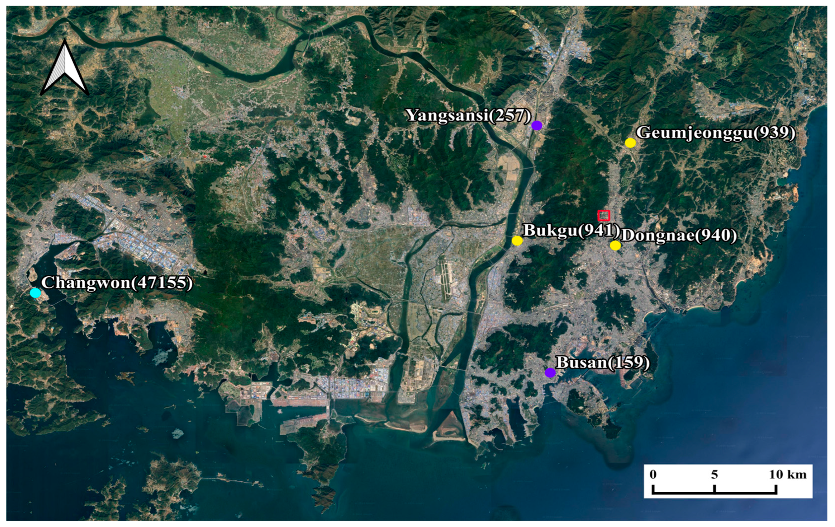
A research area was selected at the Pusan National University (PNU) campus in Geumjeong-gu, Busan, South Korea, based on the feasibility of data acquisition, as well as terrain and land use complexity. The valley-shaped topography of this site made it more vulnerable to UHI effects than other areas of Busan (Figure 1). Busan is a coastal city surrounded by Geumjeong Mountain, but its urban areas cover 94.7% of its land, resulting in higher surface temperatures than those in other suburban areas. Because the PNU campus is located on the hillside of Geumjeong Mountain, mountain breezes strongly influence the local climate. It consists of uplifted granite bodies containing minerals such as granodiorite, biotite granite, adamellites, and tonalite. The study area is 0.81 km2, composed of buildings, forests, ground, and roads (Figure 1). The annual mean temperature was 14.6 °C, with maximum and minimum temperatures of 36.4 °C and −11.6 °C, respectively. The annual precipitation was 2203.5 mm in 2023, and rainfall events were mostly concentrated in July and August.

2.2. Topographic and Meteorological Data

To simulate local climate variations, we divided our study area into 30 × 30 grid cells spaced 30 m apart. This increased the computation speed, allowing for the intensification of analyses and increasing the efficiency of analyses when implementing various observations in temperature modeling. Digital elevation model data were obtained from the one-arc-second Shuttle Radar Topography Mission of the United States Geological Survey [21]. Land use data were retrieved from the land-cover map of the Environmental Geographic Information Service [22].
Surface condition data were obtained from the KMA Weather Data Service using automatic weather stations (AWSs) and automated synoptic observation system (ASOSs). Rawinsonde data on upper-air meteorological conditions were obtained from the KMA website [23]. The measurements from stationary meteorological stations were represented by five meteorological stations. The AWS sites at Geumjeonggu (939), Dongnae (940), and Bukgu (941) were located near the study area. An ASOS point at Busan (159) was chosen to assess the impact of urban and coastal climates, and an ASOS point in Yangsansi (159) was used to model mountainous climate. Data from the Changwon (47155) station were used to calculate upper-air meteorological parameters (Figure 2).

2.3. Heat Balance Considerations

The heat balance equation for the meteorological model is as follows [24]:
Q * + Q f = Q h + Q e + Q g
Q * is the net radiation flux (W/m2), Q f is the anthropogenic heat flux (W/m2), Q h is the sensible heat flux (W/m2), Q e is the latent heat flux (W/m2), and Q g is the storage/soil heat flux (W/m2).
To estimate Q * , the temperature (T) was used for the net radiation flux as follows [24]:
Q * = 1 A Q s w + c 1 T 6 σ T 4 + c 2 N 1 + c 3
Q s w = a 1 sin φ + a 2 1 + b 1 N b 2
where Q s w is the incoming short-wave radiation (W/m2), T is the measured air temperature (deg. K), A is the surface albedo, σ is the Stefan–Boltzman constant (5.67 × 10⁻⁸ W m−2 K−4), N is the fraction of the sky covered by clouds, and φ is the solar elevation angle (deg.). Net radiation constants ( a 1 ,   a 2 ,   b 1 ,   b 2 ,   c 1 ,   c 2 ,   c 3 ) can be found in [24]. a constants mean the turbidity coefficient; a 1 is 990 W/m2 and a 2 is −30 W/m2. b constants are empirical coefficients which depend on the climate of the site; b 1 is 0.75 and b 2 is 3.4. c constants are empirical coefficients that are related to radiation; c 1 is 5.31 × 10⁻¹³ W/m2/deg K6, c 2 is 60 W/m2, and c 3 is 0.12.
To compute meteorological variables, obtaining the spatial distribution of T from measurements is important to consider the spatial distribution of Q * . A combination of temperature measurements from meteorological stations and simulations from KMA were used to estimate the spatial distribution of T or a specific point of T, using inverse distance weighting interpolation. Q * in Equation (2) is a critical variable because it can be used to estimate Q g , Q h , and Q e using the Bowen ratio and constant c g representing the properties of a surface [25].
The wind velocity field effects were estimated using the terrain slope flow, kinematic terrain effects, and terrain blocking effects. Divergence minimization combined with kinematic terrain effects and terrain blocking effects resulted in the generation of three-dimensional wind velocity components (u, v, and w). Model parameters, such as surface friction velocity, convective velocity scale, Monin–Obukhov length, and mixing height, were computed using a revised two-dimensional wind velocity field (u and v). A two-dimensional wind velocity field was used to redistribute the temperature distribution. To conduct this study, we used five meteorological stations and ten boundary points obtained from the Fusion Weather Application Programming Interface (FWAPI) [26,27].

2.4. Mobile Data Implementation

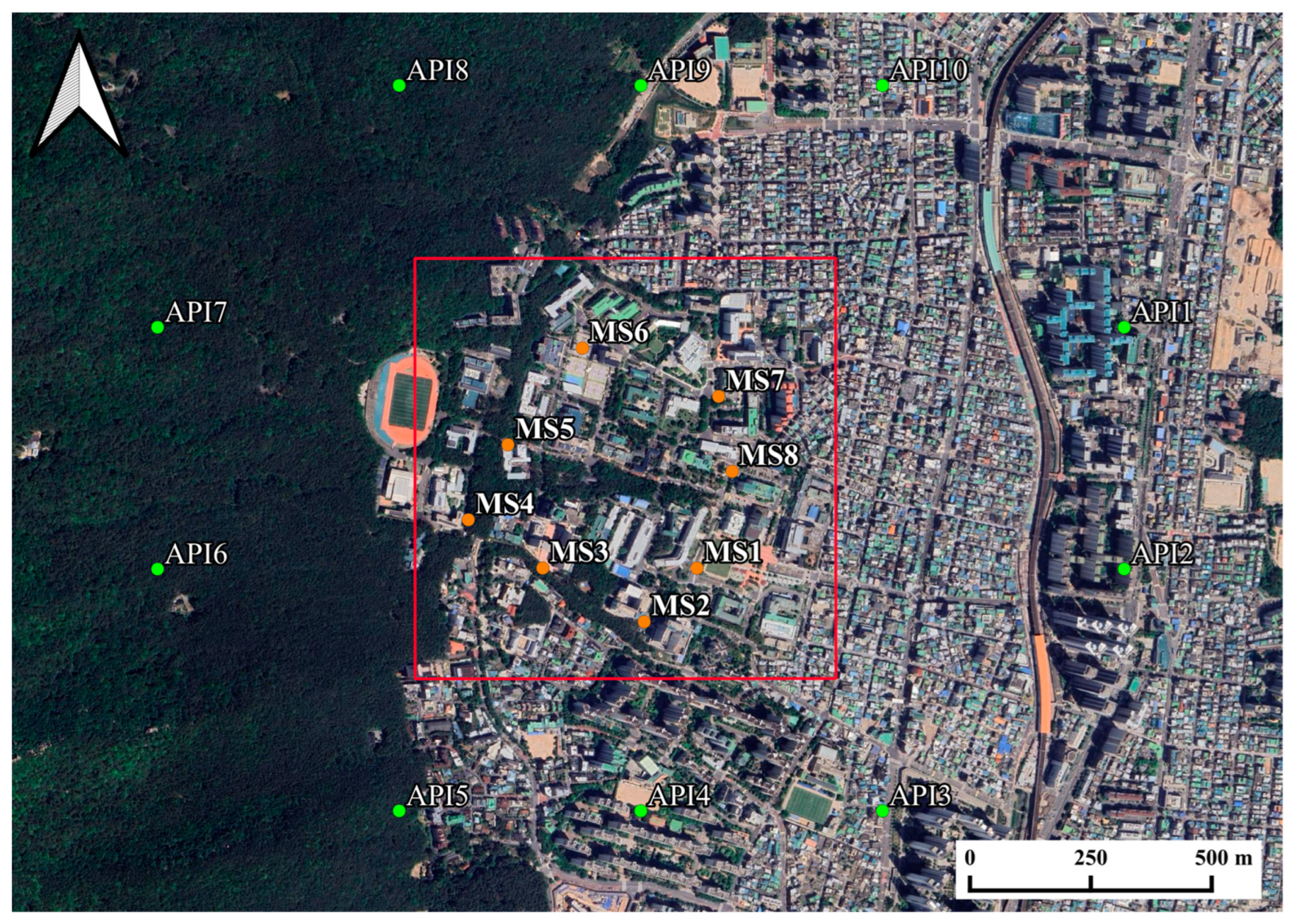
Data were collected from the study area using a mobile weather observation system (MWOS) provided by the KMA (Figure 3). As shown in Figure 4, temperature variation was measured along the mobile route (MS1 to MS8). Mobile routes have slopes ranging from 0° to 15°. MWOS temperature data can be incorporated into a model that evaluates the time series of two-dimensional temperature fields. Treating MWOS data properly (such as through interpolation or extrapolation) is necessary to fit the temperature modeling time step. However, it can be challenging to implement MWOS measurements because of the nonstationary nature of mobile data collection. Mobile and stationary measurements cannot always be precisely matched because field conditions are unpredictable [11].
In this study, the mobile measurement route and sampling locations corresponded to the spatial and temporal coordinates of the modeling and measurement. The MWOS’s unstable data feature was addressed by developing a simple mobile data implementation protocol. Meteorological data were collected by the MWOS at 0.1 Hz and were produced every minute based on the moving averages of six series of temperatures, humidity, precipitation, pressure, wind direction, and wind speed. Field data collection was conducted between 14:30 and 17:30 on 2 February 2024 in the study area. In temperature fields, an error bound of 0.3 °C can be used as a measure of accuracy.
Dataset matching between the modeling and measurement values was achieved by both adjusting the sampling locations on mobile routes and scheduling in MWOS operations. Mobile-collected data had to be converted to fit a designated grid and the corresponding time in the modeling cycle because most meteorological models rely on grid-based platforms. Data matching between the modeling and actual field data collection was achieved by adjusting the sampling locations on mobile routes and scheduling in MWOS operations. There are various possible mobile data implementation scenarios, depending on the location and timing of the data collection. On 2 February 2024, mobile data collection using the MWOS was performed for the route shown in Figure 4 between 14:30 and 17:30. To consider the concentration of buildings at lower elevations, we selected points MS1, MS2, MS3, MS7, and MS8 along the route. Mountainous and high-elevation regions were represented by MS4, MS5, and MS6. A wide, open area of sunlight dominated point MS1, whereas dense foliage covered point MS5. For stations MS1 and MS8, the MWOS stopped for six minutes after traveling at 20–25 km/h [12]. Data collection was performed hourly, with three to four observations per point.
Twenty-three field data implementation points were identified, including five meteorological data points from meteorological stations, ten FWAPI points for outer boundary impacts, and eight mobile data points using the MWOS. Modeling was performed using all 23 datasets, which were defined as the Modeling Result with Total dataset (MRT). Each combination of possible data consideration cases was converted into its corresponding data structure, which was then used as an input for modeling. Mobile data implementations can be created based on a dataset of 15 measurements (five from the AWS and ASOS, and ten from the API). A point mobile dataset was designed using fifteen measurement datasets, and one of the eight mobile datasets was used to indicate the modeling using 16 field measurement datapoints. In addition, 255 possible data implementation scenarios could be delineated (Table 1).
The integration of meteorological stations and mobile devices has not yet been explored in meteorological modeling. Mobile data scenarios are often considerably affected by mobile data implementation. Therefore, we compared the MRT and 255 combinations in terms of modeling performance. The modeling differences between the MRT and one of the two hundred and fifty-five combinations were evaluated in terms of the mean, maximum, minimum, standard deviation, and root mean square error (RMSE). By considering the monitoring device error bound, this procedure can provide results for an efficient measurement campaign when integrating mobile data into existing meteorological modeling platforms (model + meteorological stations). It is possible to minimize the redundancy of mobile data collection campaigns by considering the spatial and temporal distributions of temperature and its measurement error bound.

3. Results

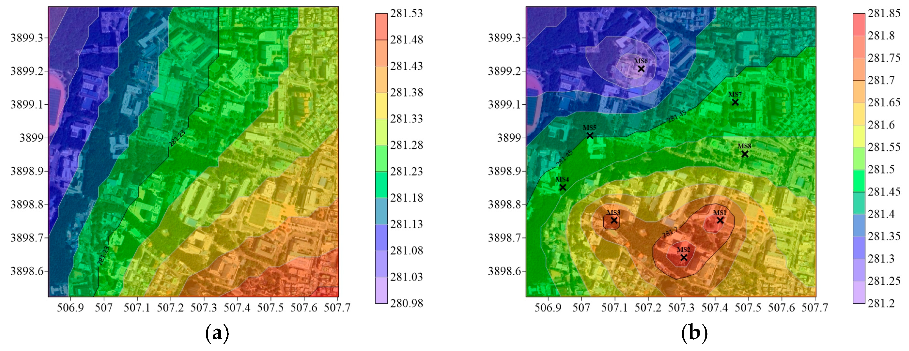
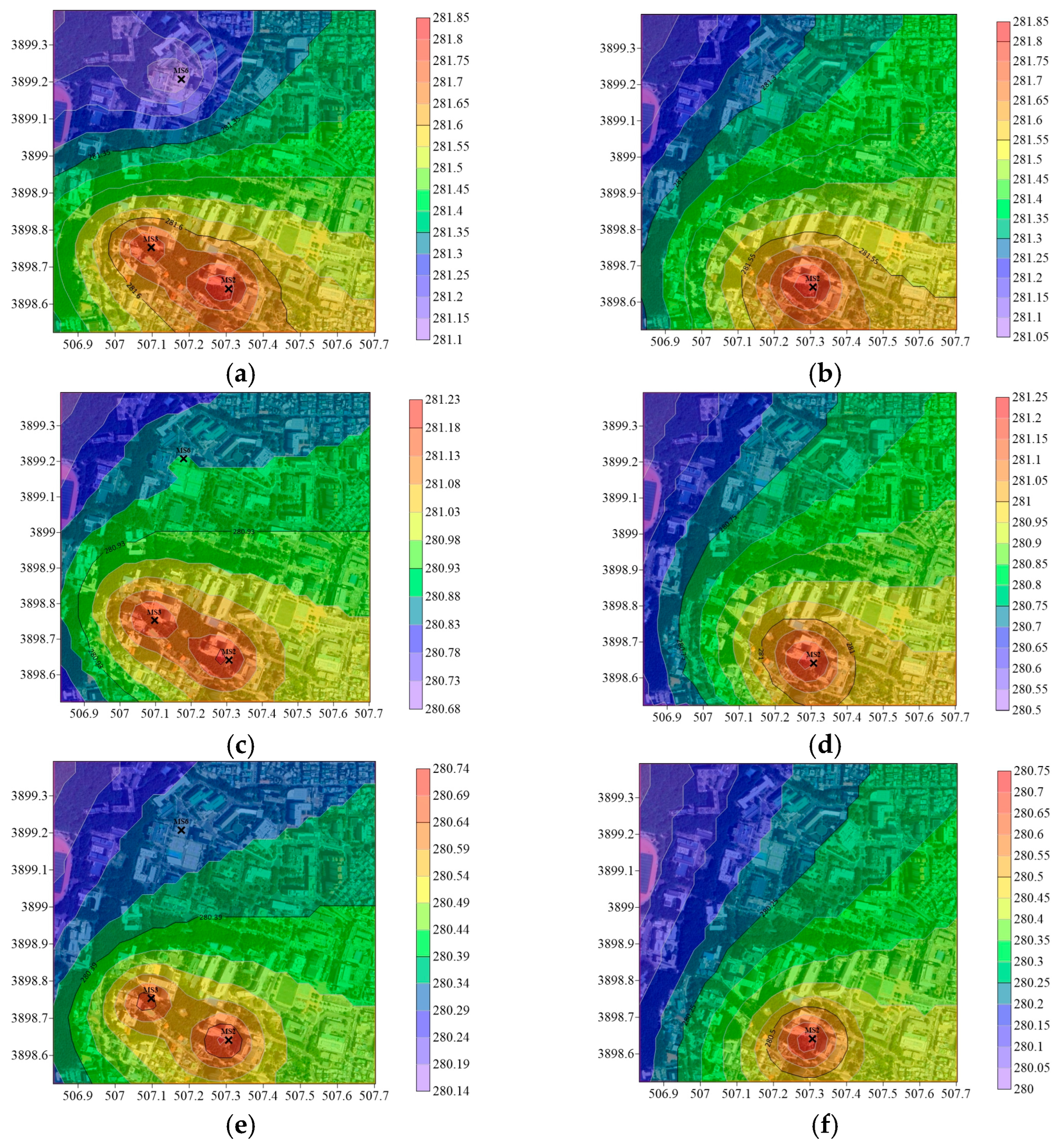
Figure 5a shows the meteorological modeling of temperature at 15:00 on 2 February 2024. This was based on measurements from five meteorological stations and ten FWAPI stations. MS_0 in Figure 5a indicates that no mobile data were included in the modeling results. Figure 5a shows temperatures ranging from 280.98 to 281.52 K, with a downslope gradient from northwest to southeast. The role of FWAPI as a boundary condition contributed to the smooth curvature of the temperature variation. Figure 5c shows that the temperature distribution at 16:00 on 2 February 2024 had less variation than that in Figure 5a, and the downslope gradient shifted in the east–west direction. As shown in Figure 5e, the temperature distribution was even narrower at 17:00 than one hour prior (Figure 5c). Figure 5a,c,e consecutively show that the mountainous terrain from the western boundary had a stronger impact, while temperature disturbances (higher temperatures), which caused the concentration of buildings in the southeast corner, tended to disappear later. Mountain breezes blowing on Geumjeong Mountain’s eastern side during the late afternoon may explain this phenomenon [28].
Temperature models using the MRT for 15:00, 16:00, and 17:00 are shown in Figure 5b,d,f, and the positions of MS1–MS8 are marked with x. Figure 5a,b show the differences between the cases without and with mobile measurements. The temperature distribution in Figure 5b shows that the highest-temperature region lay in the southern part, and the lowest-temperature region lay in the northern part. As shown in Figure 5b, the maximum temperature was approximately 0.3 K higher than that in Figure 5a, and a saddle-shaped contour in temperature was observed at mobile observation points MS1, MS2, and MS3. In addition, the spatial temperature gradient was different at 16:00 on 2 February 2024 (Figure 5c,d). Based on the peaks of MS1, MS2, and MS3, Figure 5c shows a west-to-east gradient, whereas Figure 5d shows a northwest-to-southeast gradient. The simulation at 17:00 revealed a temperature range of 280.22–280.64 K, as shown in Figure 5f. MS1’s temperature decreased more rapidly than that of its previous time step, and singular points formed near MS2 and MS3. MS1 had a wider area, which accounted for a greater variation in the local temperature than MS2 and MS3, which had more densely populated areas. In Figure 5f, the temperature gradient from north to south was evident at locations MS7 and MS8, where the temperature decreased more rapidly.
The use of mobile temperature measurements in modeling can result in distinct differences in the temperature distribution, not only for the local area as a singular contour, such as heavily concentrated buildings, but also spatially and temporally for temperature distribution gradients, as shown in Figure 5b,d,f. For accurate temperature simulation in urban environments, considering mobile temperatures obtained inside a study area is necessary for micrometeorological modeling.
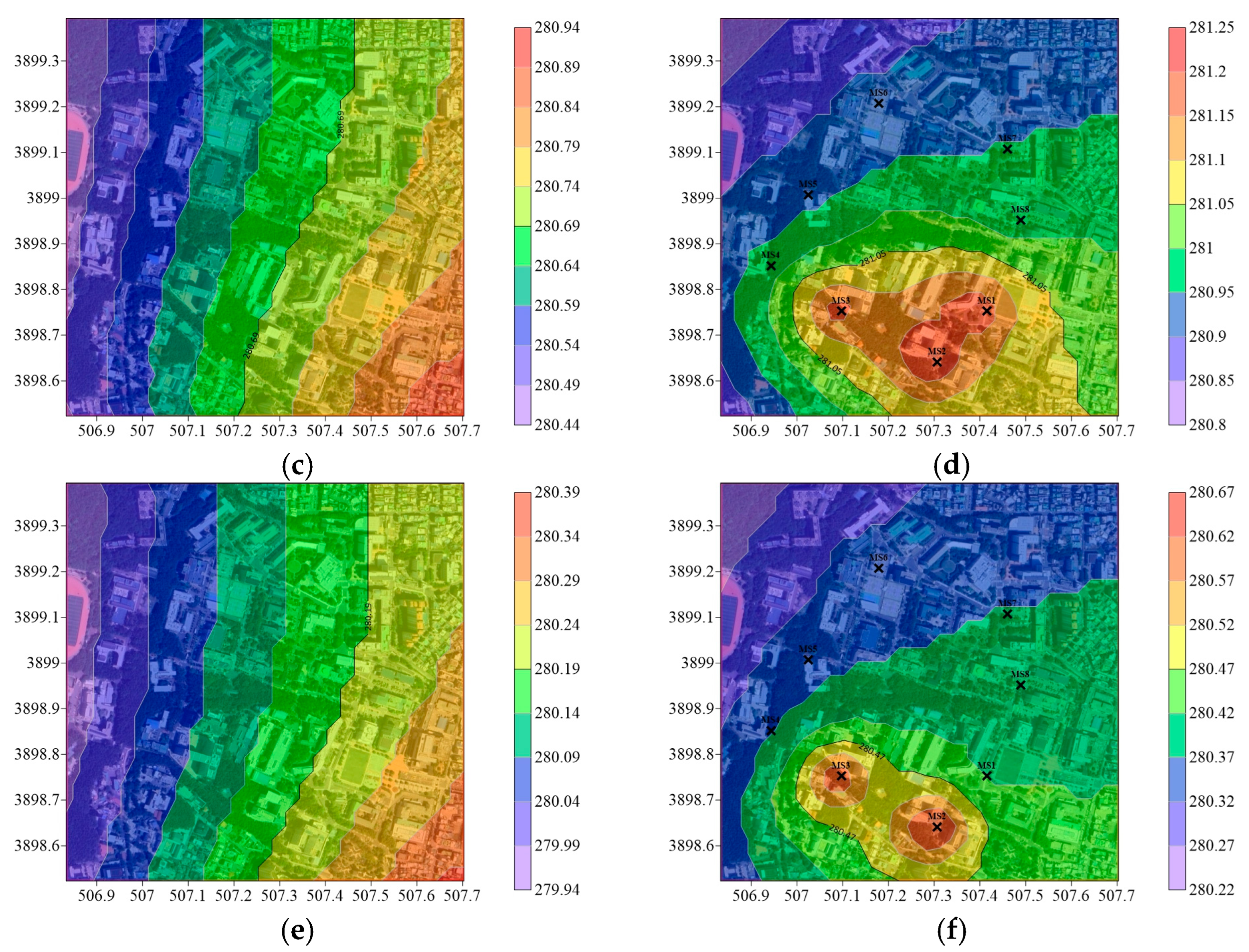
As shown in Table 1, mobile measurements could be obtained from multiple datasets, and 255 combinations could be modeled. Using the measurements from MS2, MS3, and MS6, Figure 6a shows the temperature modeling for 15:00. The temporal distributions in Figure 6a are similar to those in Figure 5b, despite MS_3 having a lower number of mobile data than the MRT. An exception occurred at MS1, where the temperature was higher (Figure 6a) than that at the MRT (Figure 5b). According to Figure 5b, the missing data for MS4, MS5, MS7, and MS8 in MS_3 appeared to have little effect on Figure 6a. According to Figure 6c, the temperature distribution for MS_3 at 16:00 was similar to that in Figure 5d; however, the local temperature features for the missing MS1 also differed. A comparison of the MRT and MS_3 at 17:00 revealed no significant differences (see Figure 5f and Figure 6e). The mobile measurements of MS1 at 17:00 showed no significant differences from those at its northern points. There was a general similarity in the spatial distributions of temperature between the MRT and MS_3. This was explained by the fact that points MS2, MS3, and MS6 adequately represented the local characteristics of the temperature.
Figure 6b,d,f illustrate the temperature modeling between 15:00 and 17:00, obtained using mobile point MS_1 as reference point MS2. However, the overall temperature curves for MS_1 matched those for the MRT, despite the absence of high-temperature contours in M1 and M3. Therefore, mobile data should be implemented with location and timing in mind to reduce costs and maintain adequate modeling results.
A comparison could be made between the MRT and 255 partial dataset combinations based on the differences in their temperature models. It was possible to evaluate the impact of mobile data on modeling using meteorological data (10 + 5) by comparing the differences between MRTs (Figure 5b,d,f) and MS_0 (Figure 5a,c,e). Differences were calculated in terms of the mean, maximum, minimum, standard deviation, and RMSE.
For identical time periods, the MRT and MS_0 could be compared to assess the impact of mobile data implementation on modeling (Figure 5a–f). During the time period 15:00–17:00, the maximum differences were 0.47, 0.55, and 0.51 °C, exceeding the 0.3 °C error bound for points MS1, MS2, and MS3. Minimum temperature differences were found near hillsides in mountainous regions, ranging from 0.04 to 0.16 °C. Average temperature differences ranged from 0.25 to 0.33 °C, with standard deviations ranging from 0.081 to 0.088. RMSEs ranged from 0.25 to 0.34 °C, which were more or less consistent with the error bound.
Among the two hundred and fifty-five combinations of mobile data, three modeling scenarios are presented in Table 2. MRT-MS_3 (236) in Table 2 shows mean differences of 0.0068, 0.047, and −0.0085 from 15:00 to 17:00 and maximum differences of 0.21 and 0.16 °C for 15:00 and 16:00, respectively. Statistically, MRT-MS_3 (236) was less than 0.3 °C, and the temperature difference at 17:00 was negligible. The temperature difference statistics for MRT-MS_4 (5678) showed 10 times higher mean differences, specifically 0.1916, 0.1884, and 0.1280 °C, for 15:00 to 17:00 than those for MRT-MS_3 (236), which had maximum differences of 0.41, 0.41, and 0.38 °C, exceeding the error bound of 0.3 °C. The RMSEs for MRT-MS_4 (5678) were three to four times higher than those for MRT-MS3 (236). This was because noteworthy measurements from the southern building area were not incorporated into the model. The difference statistics between MRT and MS_1 (2) also showed lower maximums, 0.23, 0.28, and 0.29 °C. Furthermore, the MRT-MS_4 (5678) results showed lower mean, minimum, and RMSE values than those for MRT-MS1 (2). The RMSE difference between MRT-MS_1 (2) and MRT-MS_4 (5678) was substantial at 15:00, but it was reduced at 16:00 and 17:00 because of a stronger mountain breeze. All the statistics of MRT-MS_1 (2) demonstrated better simulation results than those of MRT-MS_4 (5678). Mobile measurements were most effective when sampling points were located and scheduled to address the specific characteristics of temperature distributions rather than the number of measurements taken.
For mobile campaigns, considering the locality of mobile temperature implementation as a key factor is also important (Table 2). Considerations of notable land uses, such as the concentrated buildings in this study, can greatly benefit microclimate modeling for urban environments.

4. Discussion

Mobile platforms have been used in numerous studies to obtain better field temperature data [11,29,30], or they have used mobile devices combined with stationary meteorological stations [31,32]. Based on field measurements, most studies have used statistical methods (such as co-kriging and inverse interpolation) to investigate the spatial and temporal distributions of temperature. For statistical calculations, however, the distance between sensing points appears to be the primary weighting driver, which provides a feasible method for filling in missing measurements. This technique is feasible if the spatial features (e.g., elevation, land use, and texture) of a study area are uniform. Many materials with different heat-reacting properties can be used in typical urban areas. Temperature distribution can also be affected by complex terrains (e.g., topography or building heights). To address this issue, a physics-based micro-meteorological model was used to effectively combine temperature measurements from the MWOS and meteorological stations. A meteorological model was used to calculate the spatial distribution of heat balance and its two-dimensional wind fields. The temperature measurements from MWOS and boundary stations were redistributed using a temporally renewed wind field.
Compared with existing approaches, this method has two noteworthy advantages. The temperature fields of the study area were delineated based on heat balance processes. Land use, texture, and terrain impacts were considered when calculating the temperature field. Therefore, changes in land use or texture may be incorporated into the developed method to re-evaluate temperature fields. Meteorological modeling-based methods, in contrast to statistical interpolation, can provide physical explanations for the computed temperature fields. These notable spatial features provide an opportunity to design effective mobile campaigns. As shown in Figure 5a and Figure 6f and Table 2, the importance of mobile implementation is determined not by the number of sampling points but by the local feature, which addresses the location-based aspect. The inclusion of important local measurements into the modeling process may greatly improve the accuracy of field evaluations within the error bounds of measurement sensors, although further delicate calibration for local modeling parameters may be another important research topic.

5. Conclusions

AWS and ASOS meteorological data, FWAPI simulations, and a mobile platform (MWOS) were used to model temperature in urban environments. A physics-based meteorological process was used to simulate the temperature over three consecutive hours, using 256 measurement scenarios for the MWOS. To assess the contribution of each mobile campaign, the modeling results based on the total dataset (MRT) was compared with the modeling results based on partial mobile datasets. The impact of mobile data on temperature modeling was significant. The differences between the MRT and simulation without mobile data were 0.5 °C at maximum, 0.25 and 0.3 °C on average, and 0.25 and 0.35 °C in RMSE, even in the small study area, which were greater than the measurement error bound. The location and timing were found to be more important than the number of monitoring points in the mobile data analysis.
Using a mobile platform for temperature measurements, this study integrated meteorological monitoring with existing stationary measurement systems. A process-based explanation of the spatial distribution of temperature could be achieved by combining micro-meteorological models with mobile measurements. Thus, the field measurement campaign could be adjusted and modified to reduce costs without compromising the accuracy of the modeling. The study took place over three hours in a relatively small area on a university campus. Further optimization of mobile measurement campaigns, including the schedule, route, and sampling frequency, in a more complex environment over a longer period of time could be a future research topic.

Author Contributions

Conceptualization, S.K.; methodology, J.L. and S.K.; software, J.L.; validation, J.L. and S.K.; writing—original draft preparation, J.L. and S.K.; writing—review and editing, S.K.; visualization, J.L.; supervision, S.K.; project administration, S.K.; funding acquisition, S.K. All authors have read and agreed to the published version of the manuscript.

Funding

This study was supported by the National Research Foundation of South Korea (grant number 2022R1A4A5028840).

Institutional Review Board Statement

Not applicable.

Informed Consent Statement

Not applicable.

Data Availability Statement

The raw data supporting the conclusions of this article will be made available by the authors on request.

Conflicts of Interest

The authors declare no conflicts of interest.

References

  1. Tollefson, J. Ipcc climate report: Earth is warmer than it’s been in 125,000 years. Nature 2021, 596, 171–172. [Google Scholar] [CrossRef] [PubMed]
  2. Zhou, D.; Xiao, J.; Bonafoni, S.; Berger, C.; Deilami, K.; Zhou, Y.; Frolking, S.; Yao, R.; Qiao, Z.; Sobrino, J.A. Satellite remote sensing of surface urban heat islands: Progress, challenges, and perspectives. Remote Sens. 2018, 11, 48. [Google Scholar] [CrossRef]
  3. Zhou, J.; Chen, Y.; Wang, J.; Zhan, W. Maximum nighttime urban heat island (UHI) intensity simulation by integrating remotely sensed data and meteorological observations. IEEE J. Sel. Top. Appl. Earth Obs. Remote Sens. 2010, 1, 138–146. [Google Scholar] [CrossRef]
  4. Chen, X.-L.; Zhao, H.-M.; Li, P.-X.; Yin, Z.-Y. Remote sensing image-based analysis of the relationship between urban heat island and land use/cover changes. Remote Sens. Environ. 2006, 104, 133–146. [Google Scholar] [CrossRef]
  5. Chun, B.; Guldmann, J.-M. Spatial statistical analysis and simulation of the urban heat island in high-density central cities. Landsc. Urban Plan. 2014, 125, 76–88. [Google Scholar] [CrossRef]
  6. Mirzaei, P.A. Recent challenges in modeling of urban heat island. Sustain. Cities Soc. 2015, 19, 200–206. [Google Scholar] [CrossRef]
  7. Lin, J.; Qiu, S.; Tan, X.; Zhuang, Y. Measuring the relationship between morphological spatial pattern of green space and urban heat island using machine learning methods. Build. Environ. 2023, 228, 109910. [Google Scholar] [CrossRef]
  8. Hong, J.-W.; Hong, J.; Lee, S.-E.; Lee, J. Spatial distribution of urban heat island based on local climate zone of automatic weather station in Seoul metropolitan area. Atmosphere 2013, 23, 413–424. [Google Scholar] [CrossRef]
  9. Brandsma, T.; Wolters, D. Measurement and statistical modeling of the urban heat island of the city of Utrecht (the Netherlands). J. Appl. Meteorol. Climatol. 2012, 51, 1046–1060. [Google Scholar] [CrossRef]
  10. Gubler, M.; Christen, A.; Remund, J.; Brönnimann, S. Evaluation and application of a low-cost measurement network to study intra-urban temperature differences during summer 2018 in Bern, Switzerland. Urban Clim. 2021, 37, 100817. [Google Scholar] [CrossRef]
  11. Qi, Q.; Meng, Q.; Wang, J.; He, B.; Liang, H.; Ren, P. Applicability of mobile-measurement strategies to different periods: A field campaign in a precinct with a block park. Build. Environ. 2022, 211, 108762. [Google Scholar] [CrossRef]
  12. Liu, L.; Pan, X.; Jin, L.; Liu, L.; Liu, J. Association analysis on spatiotemporal characteristics of block-scale urban thermal environments based on a field mobile survey in Guangzhou, China. Urban Clim. 2022, 42, 101131. [Google Scholar] [CrossRef]
  13. Merbitz, H.; Fritz, S.; Schneider, C. Mobile measurements and regression modeling of the spatial particulate matter variability in an urban area. Sci. Total Environ. 2012, 438, 389–403. [Google Scholar] [CrossRef]
  14. Tsin, P.K.; Knudby, A.; Krayenhoff, E.S.; Ho, H.C.; Brauer, M.; Henderson, S.B. Microscale mobile monitoring of urban air temperature. Urban Clim. 2016, 18, 58–72. [Google Scholar] [CrossRef]
  15. Taha, H.; Levinson, R.; Mohegh, A.; Gilbert, H.; Ban-Weiss, G.; Chen, S. Air-temperature response to neighborhood-scale variations in albedo and canopy cover in the real world: Fine-resolution meteorological modeling and mobile temperature observations in the Los Angeles climate archipelago. Climate 2018, 6, 53. [Google Scholar] [CrossRef]
  16. Scire, J.S.; Robe, F.R.; Fernau, M.E.; Yamartino, R. A User’s Guide for the CALMET Meteorological Model. 2000. Available online: https://www.calpuff.org/calpuff/download/CALMET_UsersGuide.pdf (accessed on 4 October 2024).
  17. Grell, A.; Dudhia, J.; Stauffer, D. A Description of the Fifth-Generation Penn State/NCAR Mesoscale Model (MM5); University Corporation for Atmospheric Research: Boulder, CO, USA, 1994. [Google Scholar] [CrossRef]
  18. Skamarock, W.C.; Klemp, J.B.; Dudhia, J.; Gill, D.O.; Liu, Z.; Berner, J.; Wang, W.; Powers, J.G.; Duda, M.G.; Barker, D.M.; et al. A description of the advanced research WRF version 4. NCAR Tech. Note Ncar/Tn-556+ Str 2019, 145. [Google Scholar] [CrossRef]
  19. Rzeszutek, M. Parameterization and evaluation of the CALMET/CALPUFF model system in near-field and complex terrain-terrain data, grid resolution and terrain adjustment method. Sci. Total Environ. 2019, 689, 31–46. [Google Scholar] [CrossRef]
  20. Arregocés, H.A.; Rojano, R. Sensitivity of the CALMET-CALPUFF model system on estimating pm10 concentrations at a mining site in northern Colombia. Case Stud. Chem. Environ. Eng. 2023, 8, 100402. [Google Scholar] [CrossRef]
  21. United States Geological Survey. Available online: https://earthexplorer.usgs.gov/ (accessed on 10 September 2024).
  22. Korea Ministry of Environment Environmental Geographic Information Service. Available online: https://egis.me.go.kr/intro/land.do (accessed on 10 September 2024).
  23. Korea Meteorological Administration Open MET Data Portal. Available online: https://data.kma.go.kr/cmmn/main.do (accessed on 10 September 2024).
  24. Holtslag, A.; De Bruin, H. A Simple Scheme for Daytime Estimates of the Surface Fluxes from Routine Weather Data. J. Appl. Meteorol. Climatol. 1983, 22, 517–529. [Google Scholar] [CrossRef]
  25. Oke, T.R. The energetic basis of the urban heat island. Q. J. R. Meteorol. Soc. 1982, 108, 1–24. [Google Scholar] [CrossRef]
  26. Goodin, W.R.; McRae, G.J.; Seinfeld, J.H. An objective analysis technique for constructing three-dimensional urban-scale wind fields. J. Appl. Meteorol. Climatol. 1980, 19, 98–108. [Google Scholar] [CrossRef]
  27. Yocke, M.A.; Liu, M.K. Modeling Wind Distributions over Complex Terrain; Environmental Monitoring Systems Laboratory: Las Vegas, NV, USA; Office of Research and Development: Washington, DC, USA; US Environmental Protection Agency: Washington, DC, USA, 1979. [Google Scholar]
  28. Christopherson, R.W. Geosystems: An Introduction to Physical Geography; Simon & Schuster Books for Young Readers: New York, NY, USA, 1858. [Google Scholar]
  29. Rodríguez, L.R.; Ramos, J.S.; de la Flor, F.J.S.; Domínguez, S.Á. Analyzing the urban heat island: Comprehensive methodology for data gathering and optimal design of mobile transects. Sustain. Cities Soc. 2020, 55, 102027. [Google Scholar] [CrossRef]
  30. Kousis, I.; Pigliautile, I.; Pisello, A.L. Intra-urban microclimate investigation in urban heat island through a novel mobile monitoring system. Sci. Rep. 2021, 11, 9732. [Google Scholar] [CrossRef] [PubMed]
  31. Shi, R.; Hobbs, B.F.; Zaitchik, B.F.; Waugh, D.W.; Scott, A.A.; Zhang, Y. Monitoring intra-urban temperature with dense sensor networks: Fixed or mobile? An empirical study in Baltimore, MD. Urban Clim. 2021, 39, 100979. [Google Scholar] [CrossRef]
  32. Sun, C.-Y.; Kato, S.; Gou, Z. Application of low-cost sensors for urban heat island assessment: A case study in Taiwan. Sustainability 2019, 11, 2759. [Google Scholar] [CrossRef]
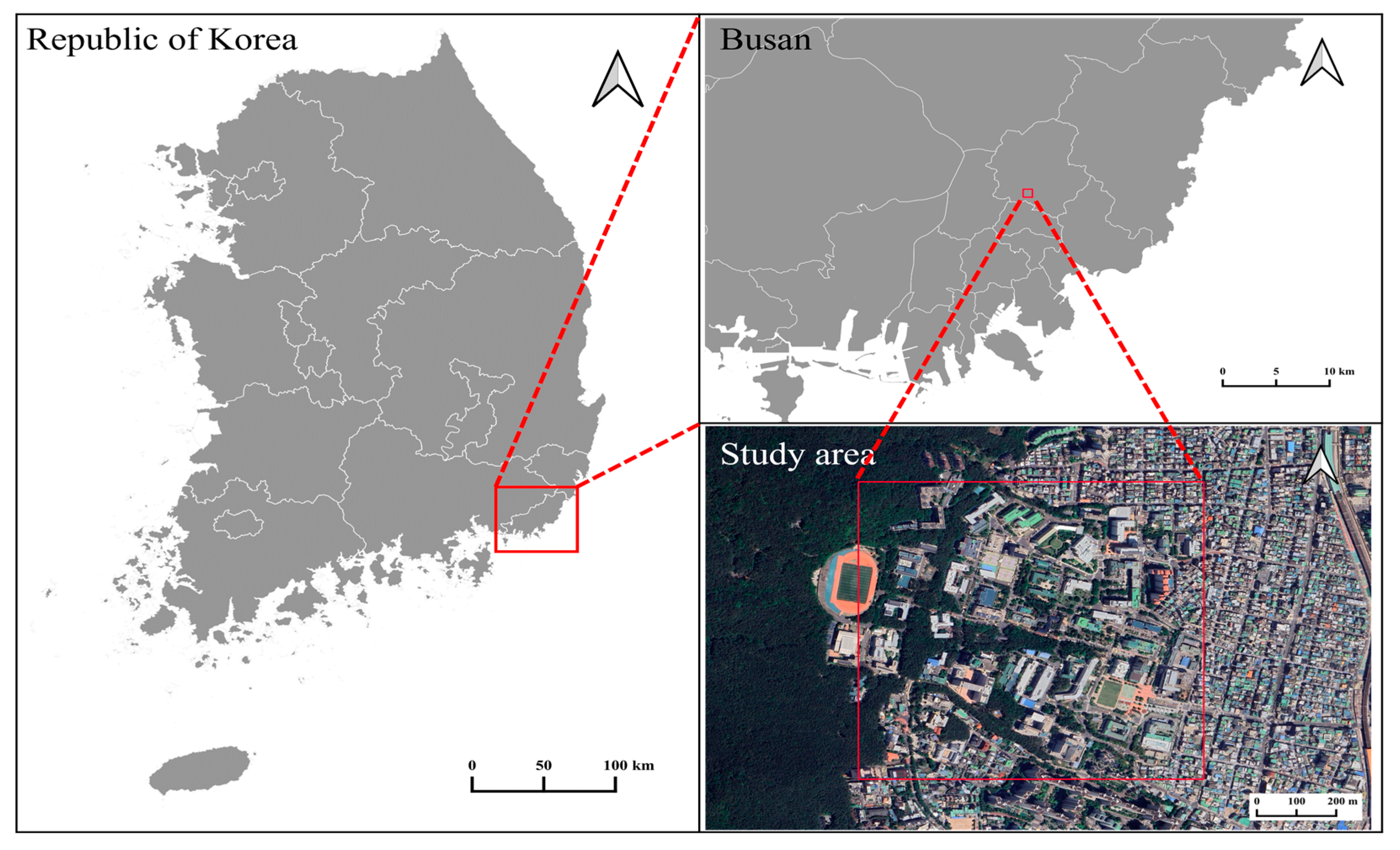
Figure 1. Geographical locations and study area in Busan, South Korea.
Sustainability 16 08897 g001
Figure 2. Locations of meteorological stations used for the study area.
Sustainability 16 08897 g002
Figure 3. Mobile weather observation system of the Korea Meteorological Administration.
Sustainability 16 08897 g003
Figure 4. Measurement locations of MWOS (MS1 to MS8) and API boundary locations (API 1 to API 10).
Sustainability 16 08897 g004
Figure 5. Temperature models (deg. K) (MS_0) using measurements from meteorological stations (AWS, ASOS, and API) from 15:00 to 17:00 on 2 February 2024 (a,c,e), and those for measurement from meteorological stations and the total dataset of the MWOS (MRT) from 15:00 to 17:00 on 2 February 2024 (b,d,f).
Sustainability 16 08897 g005aSustainability 16 08897 g005b
Figure 6. Temperature models (K) using measurements from meteorological stations (AWS, ASOS, and API) and three mobile measurement points (MS2, MS3, and MS6; MS_3 (236)) from 15:00 to 17:00 on 2 February 2024 (a,c,e) and those for measurement from meteorological stations and a mobile measurement point MS2 (MS_1[2)]) from 15:00 to 17:00 on 2 February 2024 (b,d,f).
Sustainability 16 08897 g006
Table 1. Combinations of mobile datasets for different numbers of mobile stations.
Number of Mobile Point ImplementationsNumber of Mobile Data Combinations
81
78
628
556
470
356
228
18
01
Table 2. Statistics (Average: mean, Max: maximum, Min: minimum, Std: standard deviation; RMSE: root mean square error) of differences between MRT and models with combinations of partial datasets.
Statistics in DifferencesTiming
MRT-MS_015:0016:0017:00
Average0.24150.3283780.248089
Max0.470.550.51
Min0.040.160.08
Std0.08061620.08829260.083973
RMSE0.25480.3400410.261915
MRT-MS_3(236)15:0016:0017:00
Average0.06852220.0478333−0.00851111
Max0.210.160.07
Min−0.04−0.03−0.08
Std0.04293840.02680120.0334565
RMSE0.08086410.054830.0345221
MRT-MS_4(5678)15:0016:0017:00
Average0.1916560.1883890.127956
Max0.410.410.38
Min0.080.080.05
Std0.0773250.08285710.0707204
RMSE0.2066660.2058050.146198
MRT-MS_1(2)15:0016:0017:00
Average0.09223330.1638890.0993778
Max0.230.280.29
Min−0.070.02−0.06
Std0.04626510.05673320.0686541
RMSE0.1031860.1734310.120786
Disclaimer/Publisher’s Note: The statements, opinions and data contained in all publications are solely those of the individual author(s) and contributor(s) and not of MDPI and/or the editor(s). MDPI and/or the editor(s) disclaim responsibility for any injury to people or property resulting from any ideas, methods, instructions or products referred to in the content.