Article

The Real-Time Dynamic Prediction of Optimal Taxi Cruising Area Based on Deep Learning

1
College of Transportation Engineering, Chang’an University, Xi’an 710064, China
2
Key Laboratory of Transport Industry of Management Control and Cycle Repair Technology for Traffic Net-Work Facilities in Ecological Security Barrier Area, Chang’an University, Xi’an 710064, China
*
Author to whom correspondence should be addressed.
Sustainability 2024, 16(2), 866; https://doi.org/10.3390/su16020866
Submission received: 30 October 2023 / Revised: 24 December 2023 / Accepted: 17 January 2024 / Published: 19 January 2024

Abstract

:
A real-time, effective, and dynamic taxi cruising recommendation strategy is essential to solving the problem of taxi cruising passenger difficulty and urban road traffic congestion. This study focuses on two aspects of the real-time accessible range and pick-up ratio (PR) and proposes a real-time dynamic identification method for taxi optimal cruise-seeking area. Firstly, based on the cumulative opportunity method, a univariate temporal convolutional network (UTCN) accessible range dynamic prediction model is proposed to predict the real-time accessible range of taxis. Secondly, based on the gradient boosting decision tree (GBDT) model, the influencing factors with a high correlation with the PR are selected from the four dimensions of traffic characteristics, environmental meteorology, and time and space variables. Then, a multivariate univariate temporal convolutional network (MTCN) global grid PR prediction model is constructed, and the optimal taxi cruising area is identified based on the maximum PR. The results show that the taxi accessible range and PR of the same grid in different periods change with time, and based on the model comparison, the accessible range and PR prediction results of UTCN and MTCN algorithms in different periods are the best to identify the optimal cruising area of taxis in different periods. The main contribution of this study is that the proposed optimal cruising area prediction model has timeliness, accessibility, and dynamics. It can not only improve the probability of taxis receiving passengers and avoid taxis cruising aimlessly, but also solve the shortage of taxis in hotspots, thus shortening the waiting time of passengers. This provides a scientific basis for improving taxi cruising efficiency and the government’s formulation of taxi operation management policies, which can effectively promote the sustainable development of urban traffic.

1. Introduction

Due to the acceleration of urbanization, taxis, as a door-to-door urban public transport travel service, greatly facilitate the travel of residents and are an indispensable part of urban transportation. With the continuous development of the taxi industry, the problem of the difficult reception of cruising taxi drivers has become increasingly prominent, and the rapid rise in online car-hailing is also greatly impacting the traditional cruising taxi market [1,2]. In 2020, the average daily mileage of cruising taxis was 332.3 km, and the average daily passenger mileage was 202.9 km, of which nearly 40 percent became empty cruising mileage. Correspondingly, the overall average utilization rate of drivers’ passenger time was only 45.5 percent, and more than half of the time was spent on empty taxi passenger searches [3]. A large number of taxi drivers rely on experience cruising or aimless random driving on urban roads, which will not only cause the driver’s low efficiency in seeking customers, and the length of work investment is not proportional to the revenue, but also lead to the waste of taxi resources, increase urban environmental pollution, and make the busy road traffic more congested [4,5]. Therefore, how to alleviate the low operating efficiency of cruising taxis and improve the cruising efficiency of traditional cruising taxis has become one of the urgent problems to be solved.
Traffic accessibility is the basis for studying taxi cruising recommendations. At present, when domestic and foreign scholars construct taxi cruising area identification models, they mostly use vehicle GPS trajectory data to explore the influencing factors of urban road traffic accessibility and regional accessibility [6,7]. There are two main categories of research on cruising range hotspot identification. Some scholars, to provide a better cruising search, based on a clustering algorithm [4], ant colony optimization algorithm [5], etc., obtained the hotspot area of pick-up and drop-off passengers in the whole study area, to recommend it to no-load taxi drivers. Therefore, scholars often use the pick-up ratio of the taxi in a certain area as a cruising recommendation standard [8], but this study method also has certain drawbacks. On the one hand, due to the relationship between competition and game regarding taxis, high-demand areas are often also areas where a large number of taxis gather [9,10]. Therefore, there are certain limitations in the method of directly using passenger boarding and aligning data to determine passenger hotspots. On the other hand, the research method does not limit the scope and does not consider the changes in urban hotspots in a day and the distance between drivers and hotspots [11]. Therefore, it has little reference value for the cruising decision of specific taxi drivers at a specific time.
Other scholars have defined the static search range by directly specifying the maximum search radius and simply defining the accessible range by distance [12,13]. Although this method has the advantages of simple division and easy operation, it does not consider the changes in road network accessibility caused by real-time road traffic changes. For example, within the designated radius, if the road condition is more congested, it may take a long time to reach the accessible area, which will affect the driver’s cruising efficiency. At this time, the conveniently accessible area beyond the designated range is not recommended, which is not in line with the actual reception passengers of taxis [1,6,13]. In particular, during traffic congestion periods such as morning and evening rush hours, the static range is too large, resulting in a higher time cost for drivers to travel to the recommended area [11]. However, in the middle of the night, when the traffic volume is small, the driver can reach a longer distance at the same time. At this time, the static range is too small, which leads to the recommendation that the driving area is too cautious, resulting in a smaller cruising range, and the driver may miss a certain number of pick-up passenger opportunities [12]. As can be seen, the above two types of research are of certain significance for decision makers to understand urban needs and further formulate macro policies for urban planning and transportation development. However, they do not consider the driver driving the same length of time in different areas of the city to reach the range not being the same, and even from the same position, the flat peak and peak period to reach the distance are different. That is, it does not consider that the accessible range will change dynamically in real-time with the passage of time and the different operation conditions of space roads.
In addition, scholars have considered that taxi cruising patterns are affected by external factors such as road traffic and internal factors such as individual driver behavior, which provide a rich theoretical basis for cruise-seeking area recommendations in terms of research methods [4,14,15]. For example, Chen et al. [16] found that taxi drivers’ local search decisions are largely affected by the cumulative probability of successfully carrying passengers on the search route. A combination model based on the Logit search model and intervention opportunity model was established to explain the local customer search behavior of taxi drivers. Szeto [17] proposed an ordered binary Logit model to determine the factors that affect the decision of idle taxi drivers to enter or bypass the recommended area to understand the travel behavior of empty-taxi drivers. However, the above model also has corresponding defects in the analysis. Firstly, the selection of model input variables is not comprehensive, and the index screening criteria are vague, resulting in some redundant variables with low correlation with output variables affecting the calculation accuracy of the model and reducing the upper limit of model prediction accuracy. Secondly, based on considering the high-demand area, the relevant researchers incorporate static indicators such as population, economy, and land use into the model to improve the accuracy of the model [9,10]. However, the real-time dynamics of taxi travel demand are not considered in modeling, so the research results have low reference values for real-time cruising range recommendation. Therefore, to solve the problem of obtaining the optimal cruising area of taxis only from a certain angle such as traffic variables or spatial variables, this study takes time, space, external environment, and driver’s personal factors into account in the cruising area recommendation model, that is, to identify the optimal cruising area more accurately from multiple dimensions.
With the development of deep learning models, the commonly used time series models include a Recurrent Neural Network (RNN) [18], Long Short-Term Memory (LSTM) [19,20,21], a Gated Recurrent Unit [22,23], etc. Compared with the previous time series models, the proposed temporal convolutional network (TCN) can process the input sequence in parallel and improve the computational efficiency; stack multiple convolutional layers to capture features on different time scales to better model long-term dependencies; convolution kernels of different scales learn different feature representations to better extract local and global features in time series data [24]. In addition, with the introduction of a deep learning model informer based on a self-control mechanism, it can predict the accuracy of time series with high accuracy, but its computational complexity is high, parameter adjustment requires experience, and the number of requirements is large, and the taxi data obtained in this study only involve one month, so there is a certain inapplicability [25]. Therefore, this study chooses to use the TCN model to identify the optimal cruising area of taxis.
In summary, most of the current research on a taxi cruising passenger search does not have timeliness, accessibility, and dynamics. To fill this gap, this study proposes an optimal cruising area dynamic identification method combining the accessible range and pick-up ratio. Specifically, the primary contributions of this work are summarized as follows:
  • Firstly, based on the cumulative opportunity method, a dynamic prediction model of the real-time accessible range based on UTCN is proposed to predict the real-time dynamic accessible range of taxis. Traditional studies mostly use static indicators to predict travel hotspots in the morning and evening peaks. However, this study uses multi-source data to form a spatio-temporal data chain, which can realize the real-time dynamics of accessible range prediction.
  • Secondly, considering the four factors of traffic, time, space, and external environment, an MTCN model is constructed to predict the pick-up ratio under different periods, and the high-probability passenger hotspot area is identified as the optimal cruising area. This can improve the probability of no-loading taxis picking up passengers, avoid taxis cruising aimlessly, and reduce the cruising distance of taxis to a certain extent.
  • Finally, the dynamic identification method of the optimal cruising area is constructed by combining the global passenger pick-up ratio with the real-time accessible range. Based on the case analysis, the reliability of the deep learning algorithm used in this study is verified from the model level.
The study can further recommend efficient and appropriate cruising paths for taxi drivers, help drivers improve passenger search efficiency, solve the problem of mismatch between supply and demand of taxi travel, and further alleviate urban road traffic congestion.

2. Study Area and Data

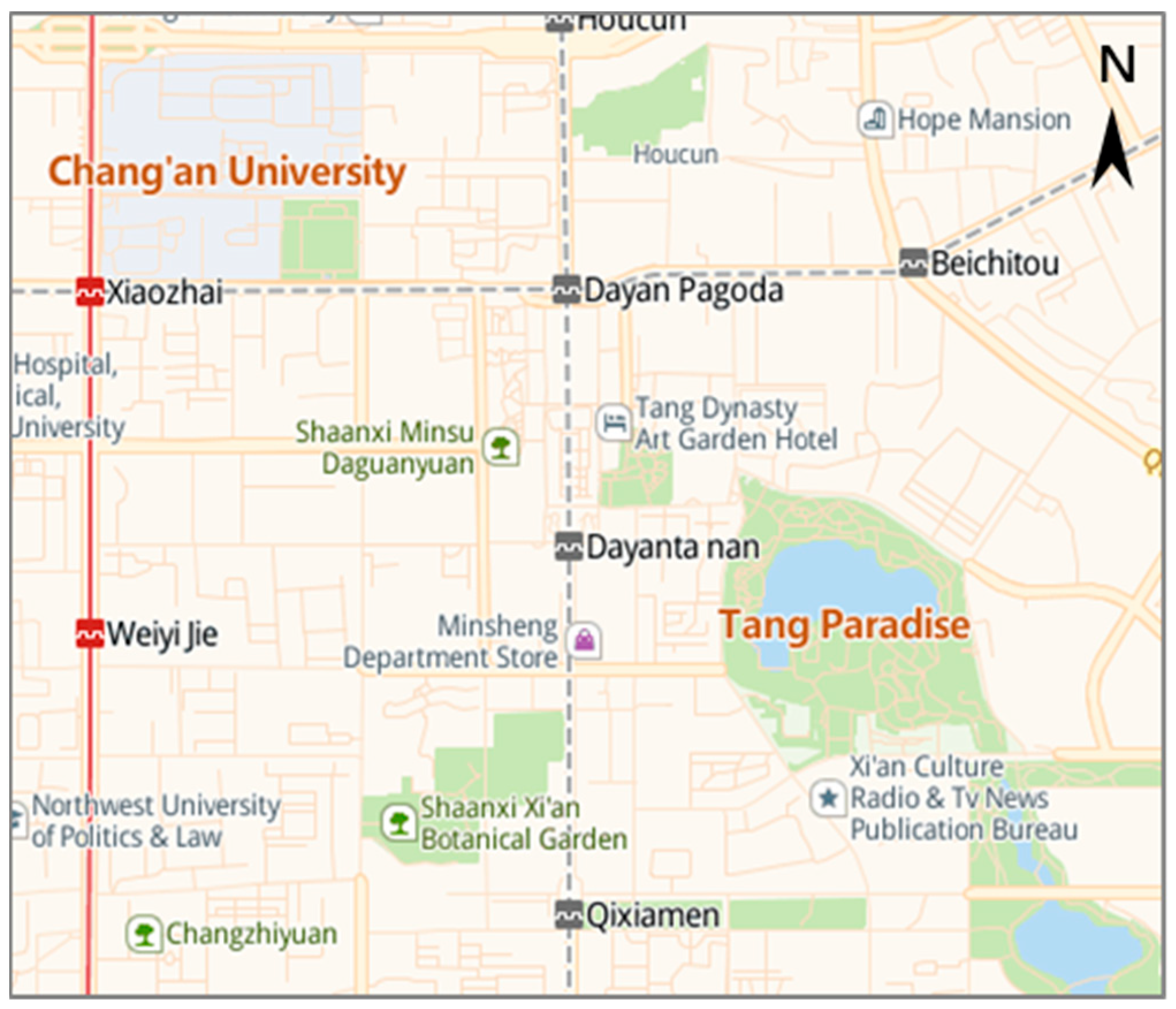
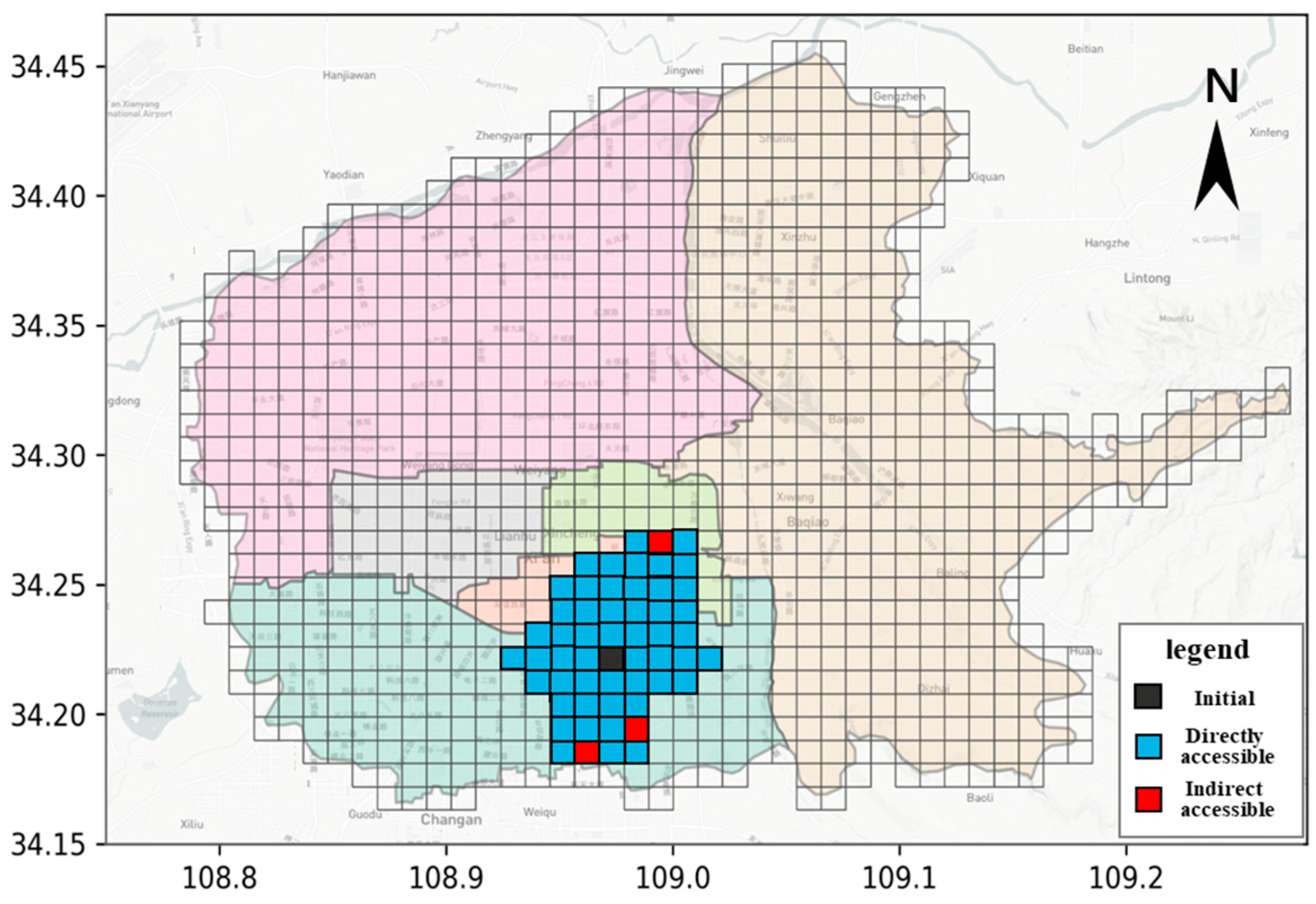
2.1. Study Area and Grid Division

Because the cruising taxi operation is mainly concentrated in the urban area, this study takes the six main urban areas of Yanta District, Beilin District, Lianhu District, Weiyang District, Baqiao District, and Xincheng District of Xi’an as the study area. As shown in Figure 1 below, the total area of the area is about 826 km2, covering the main traffic nodes such as Xi’an North Railway Station, Xi’an Railway Station, and Xi’an Bus Station, as well as important business districts such as Bell Tower and Saige International. Taking the 1 km × 1 km square as the basic unit, the central urban area of Xi’an is divided into 945 equal grids. The bottom grid of the left column is numbered as 0, and the top grid of the right column is numbered as 944, and each grid is numbered from 0 to 944.

2.2. Data Collection and Processing

The data used in this study are mainly taxi GPS trajectory data, Points of Interest (POIs) data, and meteorological data. Based on ensuring the spatio-temporal consistency of multi-source spatio-temporal data, the dynamic identification of taxi optimal passenger-seeking area is studied.

2.2.1. Taxi GPS Trajectory Data

This study selects the GPS trajectory data of taxis from 1–30 November 2019, provided by the taxi company of Xi’an, China. The average daily operating vehicles are 13,000 taxis, there are 30 million vehicle travel records per day, and the collection interval is half a minute. The original trajectory data include the license plate number, data acquisition time, longitude, latitude, speed, driving status (idle or hired), etc. The ‘0’ and ‘1’ in the taxi status field represent the idle vehicle status and the hired status, respectively. The invalid data are eliminated by preprocessing the original data, and the GPS data are sorted in chronological order. For the same vehicle license plate, when the GPS trajectory sequence is converted from ‘0′ to ‘1’, it means that the vehicle completes a pick-up operation, and the data information of state ‘1’ can be identified as the pick-up point information. On the contrary, when the GPS trajectory sequence is converted from ‘1’ to ‘0’, it means that the vehicle completes a drop-off operation, and the data information of state ‘1’ can be identified as the drop-off point information. The identified pick-up and drop-off points are matched to extract complete taxi travel data. The recognition principle is shown in Figure 2.

2.2.2. POI Data

This study uses the API of Gaode Map to crawl the POI data of the same period as the taxi trajectory data, and further screens the facilities related to residents’ travel, including 14 types of POI data [26] such as catering services, shopping services, transportation facility services, and business residences. Combining POI data with the taxi GPS trajectory can dig deeper into traffic travel demand and improve the accuracy of cruising hotspot identification.

2.2.3. Meteorological Environment Data

In this study, real-time meteorological data such as weather and air quality in the city are included in the study of taxi cruising area identification. Through the ‘Environmental cloud big data open platform’, the real-time climate data recorded by each ground observation station in Xi’an in November 2019 were obtained, including data time, weather conditions, ambient temperature, somatosensory temperature, atmospheric pressure, air humidity, wind direction, wind speed, and other indicators. Through the ‘Green respiratory data open platform’, real-time indicators of various pollutants such as AQI and PM2.5 in Xi’an in November 2019 were obtained. That is, the meteorological data are combined with the taxi trajectory to fully consider various factors affecting the taxi cruising search.

2.2.4. Spatial Matching of the Study Area and Data

The multi-source data (including GPS, POIs, and meteorological data) were spatially matched with the grid data to link into a whole, and the final data fields and data examples of the study area were obtained as shown in Table 1.

3. Methodology

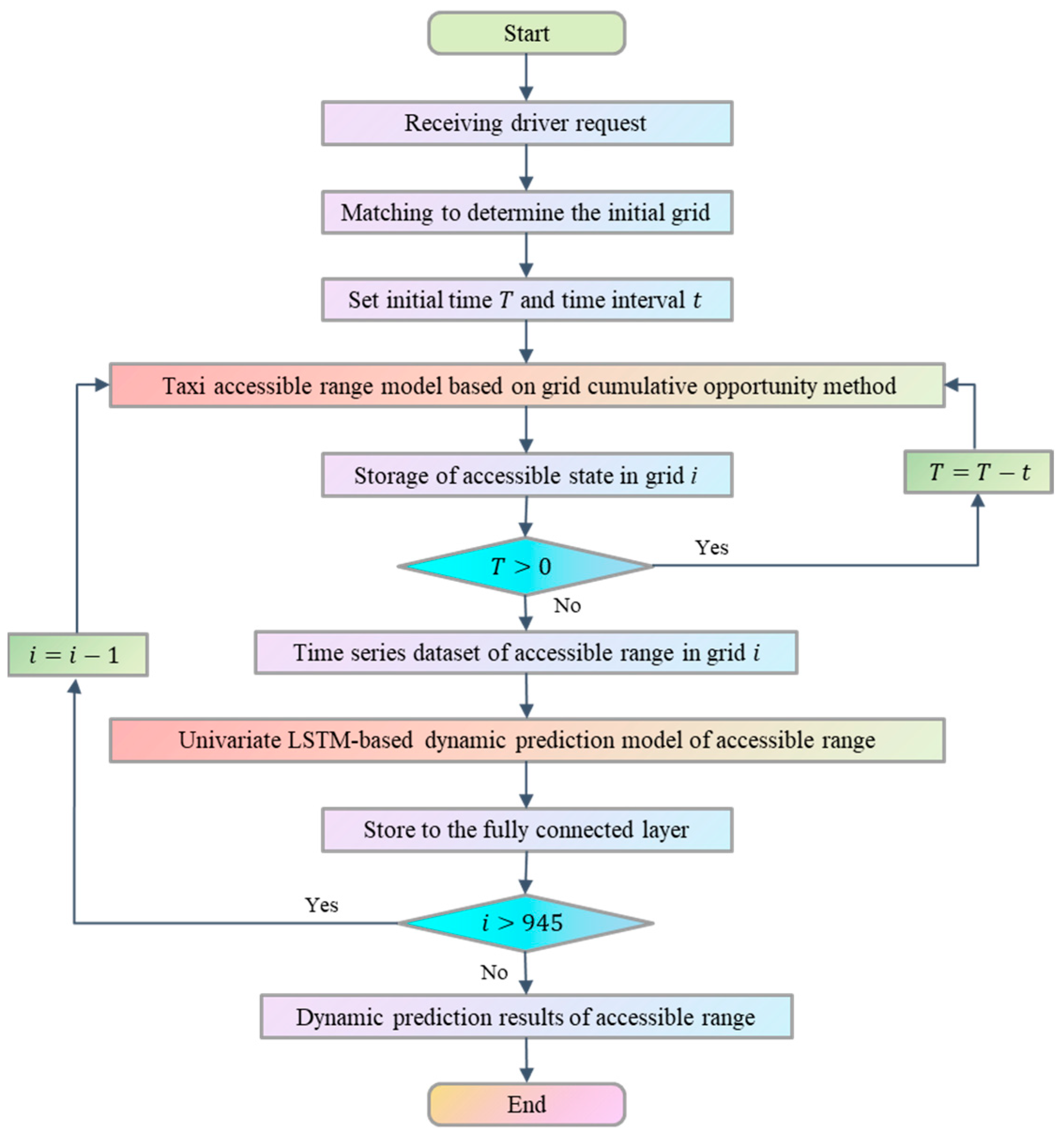
3.1. Real-Time Accessible Range Analysis and Dynamic Taxi Prediction

3.1.1. Taxi Accessible Range Determination Based on GCOM

Before identifying the optimal cruising area, the boundary range of the area needs to be prioritized. This study defines the real-time accessible range of vehicles as follows: under a given time threshold, according to the real-time vehicle trajectory, the maximum range of real-time vehicles from the current area is the real-time accessible range of vehicles. Under this definition, the accessible range of the vehicle changes in real-time with the change in time and the actual running condition of the road. This study draws on the core idea of accumulation in the cumulative opportunity method and applies it to the study of the accessible range. By accumulating the travel path of each individual, the accessible spatial range of the group starting from a certain area is obtained [14]. The grid cumulative opportunity method (GCOM) is expressed in Equation (1):
A i = j = 1 n O j t
where A i is the accessibility of region i, t is the given threshold of travel time or space, O j t is the number of opportunities in region j, and j is the region that is less than the threshold t in distance or time from region i.
The grid cumulative opportunity method example is shown in Figure 3. As shown in Figure 3a, starting from the current moment, the paths of all ride-hailing vehicles departing from grid O in a given period are I1, I2, and I3. Based on the grid cumulative opportunity method, the accessible range of taxis shown in Figure 3b can be obtained. The accessible range consists of two parts: the directly accessible range and indirectly accessible range. The former is composed of the grid range of the actual path (red line) of the taxi, and the latter comprises the range according to the travel demand of the taxi, and the indirect accessible range of the taxi can be obtained as A, B, and C. The specific traversal principle of the indirect grid is as follows: due to the relatively small amount of taxi travel in a given period, there will be a phenomenon that some grid areas have no taxis due to low travel demand, but it does not mean that taxis are inaccessible. As shown in Figure 3b, due to the low travel demand of grid A and B, there is no corresponding path through, but in the actual road network operation, taxis can reach the three adjacent grid areas of grid A and B, and they can reach the grid A and grid B areas. Meanwhile, the adjacent three grids of grid C can be reached, and grid C can also be reached. Among them, grid A and grid B are defined as indirect accessible range I, and grid C is defined as indirect accessible range II.
In summary, based on the direct accessible grid algorithm (Algorithm 1) and the grid compensation algorithm (Algorithm 2), the real-time accessible range of taxis based on the grid cumulative opportunity method can be obtained. The pseudocodes of the two algorithms are shown in below: The pseudocodes of directly accessible grid algorithm and grid compensation algorithm.
Algorithm 1: Directly Accessible Grid Algorithm.
Input: Start Grid ID, Start time, Time Interval
Output: id_set
1: licenseplates_set ← set()
2: ids_set ← set()
3: for item in data:
4:     if (id in item) and (start <= timestamp <= end) then:
5:     licenseplates_set.add(license plate)
6: for item in data:
7:     for license plate in licenseplates_set:
8:     if (license plate in item) and (start <= timestamp <= end) then:
9:     ids_set.add(id)
10: return id_set
Algorithm 2: Grid Compensation Algorithm.
Input: A two-dimensional list (Accessible id = 1, Inaccessible id = 0)
Output: Compensation grid ID
1: for x ← 0 to length_row do
2:    for y ← 0 to length_col do
3:     if grid[x][y] = 0 then
4:     if x − 1 >= 0 then
5:        a ← grid[x][y]
6:     if x + 1 < length_row then
7:        b ← grid[x + 1][y]
8:     if y − 1 >= 0 then
9:        c ← grid[x][y − 1]
10:     if y + 1 < length_col then
11:       d ← grid[x][y]
12:     if (a and b and c) or (a and b and d) or (a and c and d) or (b and c and d) then
13:       grid[x][y] ← 2
14: return grid

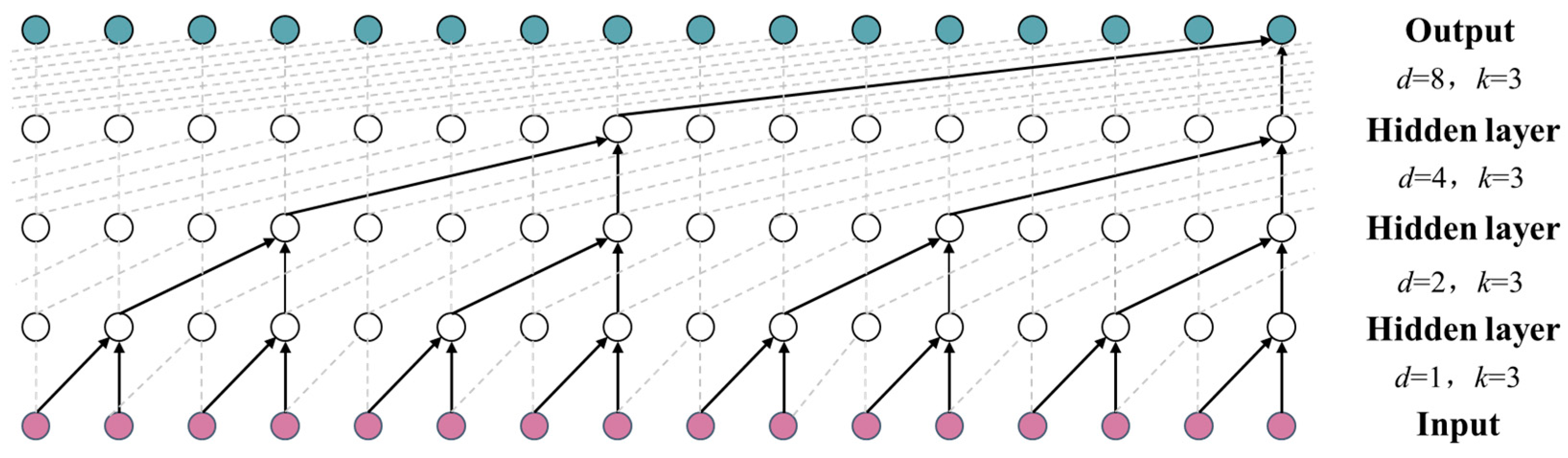
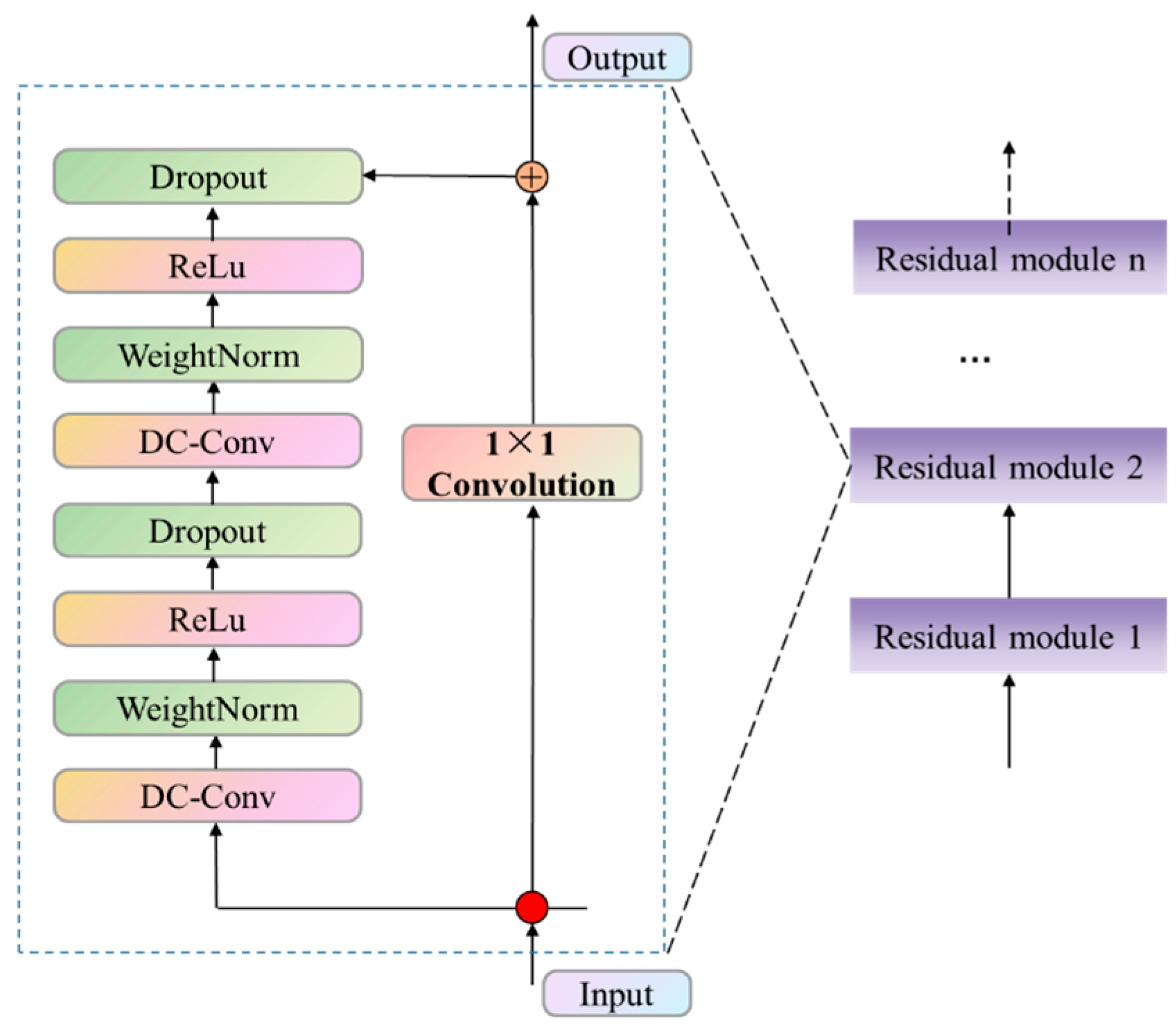
3.1.2. Accessible Range Prediction Based on UTCN

The TCN algorithm uses a one-dimensional fully convolutional network while ensuring that the network has the same input and output sequence length, introducing causal convolution, and the output at the current moment is only convoluted with the historical elements of the previous moment, to ensure that future input will not affect the prediction of past input data [24,25]. Since causal convolution will increase the number of hidden layers with the increase in the historical scale, deep networks or filters are needed to introduce dilated convolution. Figure 4 shows the expansion factor d and the filter size k. In addition, the TCN algorithm uses a residual module to solve problems such as gradient disappearance (ReLu activation function) or gradient explosion (dropout layer randomly inactivated neurons), as shown in Figure 5.
Based on obtaining the current accessible range, this study proposes a UTCN-based taxi real-time accessible range prediction model. According to Section 3.1.1, the grid number marking method is determined: the directly accessible range is marked as 1, the indirectly accessible range I area is marked as 2, the indirectly accessible range II area is marked as 3, and the inaccessible range is marked as 0.
Select the starting grid, take a certain moment as the starting time, set the time interval to 10 min, determine the historical accessible range of the taxi, construct the initial data set of the accessible range, and divide it into a training set and test set. The historical time series data set of each grid for 10 min is used as input to output the accessible state of the grid at the corresponding time in the future, that is, the numbered mark value of each grid, to predict the real-time accessible range of the grid in the research area in the next 10 min. The algorithm flow chart is shown in Figure 6.

3.2. Dynamic Prediction of Optimal Cruising Area Based on Pick-Up Ratio

3.2.1. Influencing Factor Analysis of Taxi Cruise-Seeking

Whether the driver can complete the order task quickly and successfully after receiving the order is very important to improve the vehicle utilization rate and efficiently complete the passenger transfer task. The pick-up ratio represents the degree of taxi demand in different periods in a certain area, which can reflect the operating efficiency and vehicle utilization rate of taxi drivers in a given period in a certain area. When the pick-up ratio is high, it indicates that the travel demand in this area is relatively large, and the taxi driver has a higher opportunity to carry passengers in this area, which also indicates that the vehicle utilization rate is high. Because the travel demand will change constantly in a day, such as the difference between the peak period and the low peak period, the pick-up ratio will change accordingly. As can be seen, the pick-up ratio is a key factor in identifying the final cruising area. In addition, taxi travel will be affected by many factors such as road traffic, time, spatial location, and external environment. Therefore, this study classifies the above influence factors and selects the indicators related to the taxi pick-up ratio. The specific analysis is as follows:
(1)
Traffic attribute variables
The traffic attribute variables selected in this study mainly include the pick-up ratio (PR), drop-off ratio (DR), cruising ratio (CR), heat of pick-up (HP), heat of drop-off (HD), vehicle density (VD), average operation speed (AOS). The definition and function expression of each variable are shown in Table 2.
The symbols and definitions of parameters in Table 2 are as follows: P i is the number of times that taxis located in grid i pick up passengers within a certain period; N C i is the number of idle cruising taxis in grid i within a certain period; D i is the number of times that taxis in grid i drop off passengers within a certain period; N O i is the total number of hiring taxis operating in grid i within a certain period; N i is the total number of taxis in grid i within a certain period; A i is the area of grid A; V j is the running speed of taxi j.
(2)
Time Attribute Variables
Regarding the last pick-up ratio (LPR), the passenger status of taxis at different times of the day has a certain periodicity, and the passenger demand for taxi travel changes with time [27]. For the same region, the difference between the pick-up and drop-off of passengers in the previous cycle and the next cycle is not significant. Therefore, this study considers the time periodicity and calculates the pick-up ratio of grid i on the same day and period before the last cycle in one cycle, which is defined as the LPR. The specific calculation of Equation (2) is as follows:
L P R i , t 1 , t 2 = t 1 T t 2 T P i t 1 T t 2 T N C i ,   t 1 T t 2 T N C i > 0 0 ,   t 1 T t 2 T N C i = 0
where T denotes the period length and the rest of the letters are defined as above.
The period can be selected as the day (D), hour (H), and minute (M) [28]. The specific reasons are as follows: due to the different nature of urban land in different grid areas, the travel volume of each grid on different dates in a week will also change accordingly. Therefore, the date (D) was considered as a factor affecting the taxi driver’s passenger search. For the same day, the number of people being picked up and dropped off by the taxi in each period also fluctuates regularly. Therefore, the hour (H) was selected as the influencing factor. Meanwhile, to ensure the integrity of the time attribute variables, this study also took the minute (M) as the influencing factor.
(3)
Spatial Attribute Variables
Whether taxi drivers can pick up passengers in a certain area is not only related to the traffic attribute variables and time cycle variables in the area but also closely related to the taxi demand in other areas around the area. Therefore, this study proposed the adjacent pick-up ratio (APR) index and predicted the travel demand of the target area by calculating the pick-up ratio of other areas adjacent to the target area. According to Coulomb’s law in physics, this study constructed a model of urban traffic Coulomb’s law to simulate the influence between different regions of the city [29]. Based on the regional attraction I i j , the calculation of Equation (3) is defined as follows:
A P R i , t 1 , t 2 = j = j 1 j n P R j , t 1 , t 1 × I i j j = j 1 j n I i j , j = j 1 j n I i j > 0 0 ,   j = j 1 j n I i j = 0
where grid j is the area directly adjacent to grid i, and the essence of APR is to calculate the weighted average of the pick-up ratio of each adjacent area.
(4)
Real-time Environment Attributes
According to the influence of weather on taxi cruising in previous studies [6,25], combined with the comprehensive judgment of the meteorological conditions of the period in which the data are studied in this paper, the four major environmental indicators of the weather condition (WC), apparent temperature (AT), wind speed (WS), and air quality index (AQI) were preliminarily selected as the influencing factors of taxi demand.

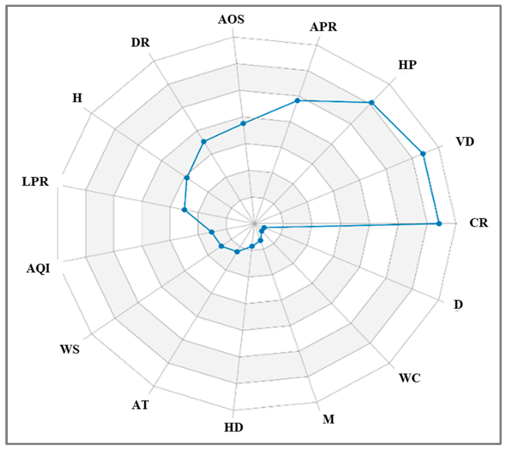
3.2.2. Variable Feature Importance Analysis Based on the GBDT Algorithm

A gradient boosting decision tree (GBDT) is a kind of ensemble learning algorithm (Figure 7), which combines a traditional boosting algorithm and decision tree [30,31]. It has the following advantages: (1) high accuracy. In each iteration, the loss function is adjusted to fit the training data step by step; (2) solving the nonlinear problem. By constructing multiple decision tree models, the nonlinear relationship of data is accurately captured; (3) handles complex features. By selecting the optimal partition feature of each node, the data set with high dimensions and complex features can be effectively processed; (4) strong interpretability. By analyzing the contribution of features, the prediction results of the model can be explained; (5) strong robustness. It is robust to noise and outliers. In the iteration, the influence of noise is weakened by fitting residuals to improve the stability of the model.
The GBDT model is constructed with the grid pick-up ratio (PR) as the output feature [32], and fifteen indicators including the drop-off ratio (DR), cruising ratio (CR), heat of pick-up (HP), heat of drop-off (HD), vehicle density (VD), average operating speed (AOS), last pick-up ratio (LPR), day (D), hour (H), minute (M), adjacent pick-up ratio (APR), weather condition (WC), apparent temperature (AT), wind speed (WS), and air quality index (AQI) as input features. The feature importance of each input index compared with the output index is analyzed.

3.2.3. Grid Pick-Up Ratio Prediction Model Based on MTCN

To ensure the real-time effectiveness of the identification and recommendation of the passenger-seeking area, it is necessary to predict the global carrying rate value at the future time through the model and dynamically recommend the optimal cruising area according to the location of the taxi at the current time. In this study, the significant variables screened using the GBDT method are used as input variables, the grid pick-up ratio (PR) is used as the output variable, and the grid is used as the research area unit to establish an MTCN-based pick-up ratio prediction model. The prediction results of all grids in the study area are further connected to measure the supply and demand level of taxis in the entire area. The pseudocode of the pick-up ratio prediction algorithm is shown below Algorithm 3: The pseudocode of the MTCN-based pick-up ratio prediction model.
Algorithm 3: MTCN-based Pick-up Ratio Prediction Model
Input: DHR, VD, RR, HP, DR, CB, OO, LM, RD, SS, BS
Output: OR
Steps:
1: import torch.nn as nn                      # Import the required libraries and packages
2: import torch. optim as optim
3: data preparation←(train_data, trainlabels,test_data,test_labels)                #Data preparation
4: class MultiVarTCN(nn.Module):                        # Define the MTCN model
5:   def __init__(self, input_size, output_size, num_channels, kernel_sizes, dropout):
6:        super(MultiVarTCN, self).__init__()
7:        self.tcn = nn.Sequential()
8:        num_layers = len(num_channels)
9:        for i in range(num_layers):
10:          if i == 0:
11:            in_channels = input_size
12:          else:
13:            in_channels = num_channels[i − 1]
14: self.tcn.add_module(‘conv{}’.format(i + 1),nn.Conv1d(in_channels,num_channels[i],
15:        kernel_sizes[i], stride = 1, padding = (kernel_sizes[i] − 1), dilation = 1))
16:           self.tcn.add_module(‘relu{}’.format(i + 1), nn.ReLU())
17:           self.tcn.add_module(‘dropout{}’.format(i + 1), nn.Dropout(dropout))
18:       self.linear = nn.Linear(num_channels[−1], output_size)
19:   def forward(self, x):
20:       out = self.tcn(x)
21:       out = out.transpose(1, 2)
22:       out = self.linear(out[:, −1, :])
23:       return out
24: data feature dimension←(input_size, output_size)             # Input and output feature dimensions
25: convolutional layer←(num_channels, kernel_sizes)
# The number of channels and the size of the convolution kernel for each convolution layer
26: other hyperparameters←(dropout, num_epochs, batch_size)
# Dropout probability, number of training iterations Batch size settings
27: model = MultiVarTCN(input_size, output_size, num_channels, kernel_sizes, dropout)
# Create the MTCN model instance
28: criterion = nn.MSELoss()                            # Loss function setting
29: optimizer = optim.Adam(model.parameters(), lr = 0.001)                 #Optimizer settings
30: data preparation←torch.from_numpy (train_data, trainlabels,test_data,test_labels)     #Convert data to Tensor
31: for epoch in range(num_epochs):                          # Cycle training model
32:      model. train()
33:      optimizer.zero_grad()
34:       outputs ← model(train_data)
35:       loss ← criterion(outputs, train_labels)
36:       loss.backward()
37:       optimizer. step()
38:       if (epoch + 1) % 10 == 0:                    # Print a loss every once in a while
39:       print(‘Epoch [{}/{}], Loss: {: .4f}’.format(epoch + 1, num_epochs, loss.item()))
40: model.eval()                                    # Model prediction
41: return predictions(OR)

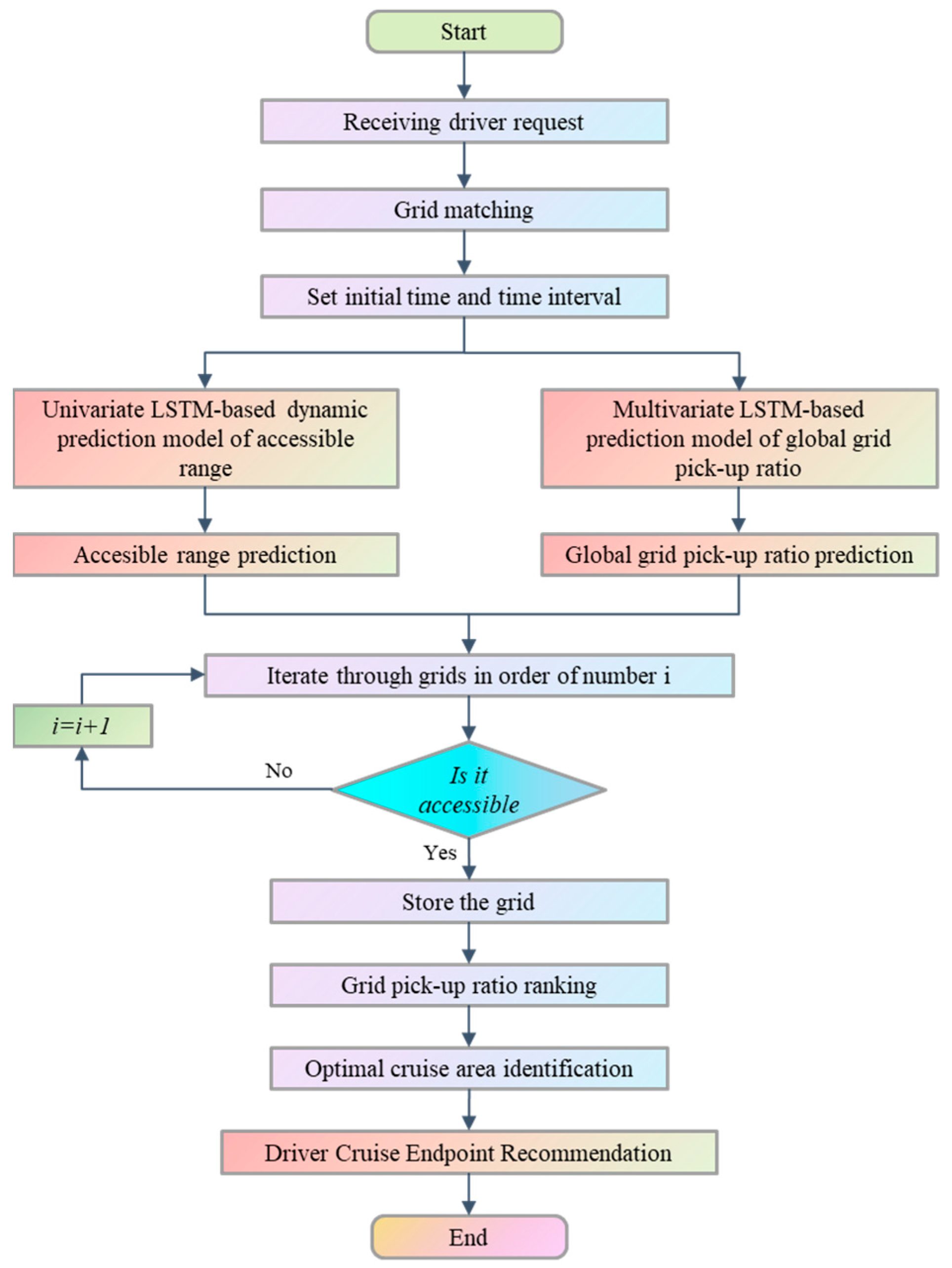
3.2.4. Optimal Cruising Area Identification Based on Accessible Range and Pick-Up Ratio

Based on the prediction of the real-time accessible range and regional grid pick-up ratio, the optimal cruising area identification strategy of taxis was formulated. The specific taxi real-time optimal cruising area identification process is shown in Figure 8.

4. Results and Discussion

4.1. Measurement Results of Real-Time Accessible Range and Pick-Up Ratio

According to the GCOM-based accessible range measurement method, this study explores the changes in the accessible range of taxi drivers starting from the same initial grid under two scenarios: different periods at the same time interval and the same period at different time intervals.

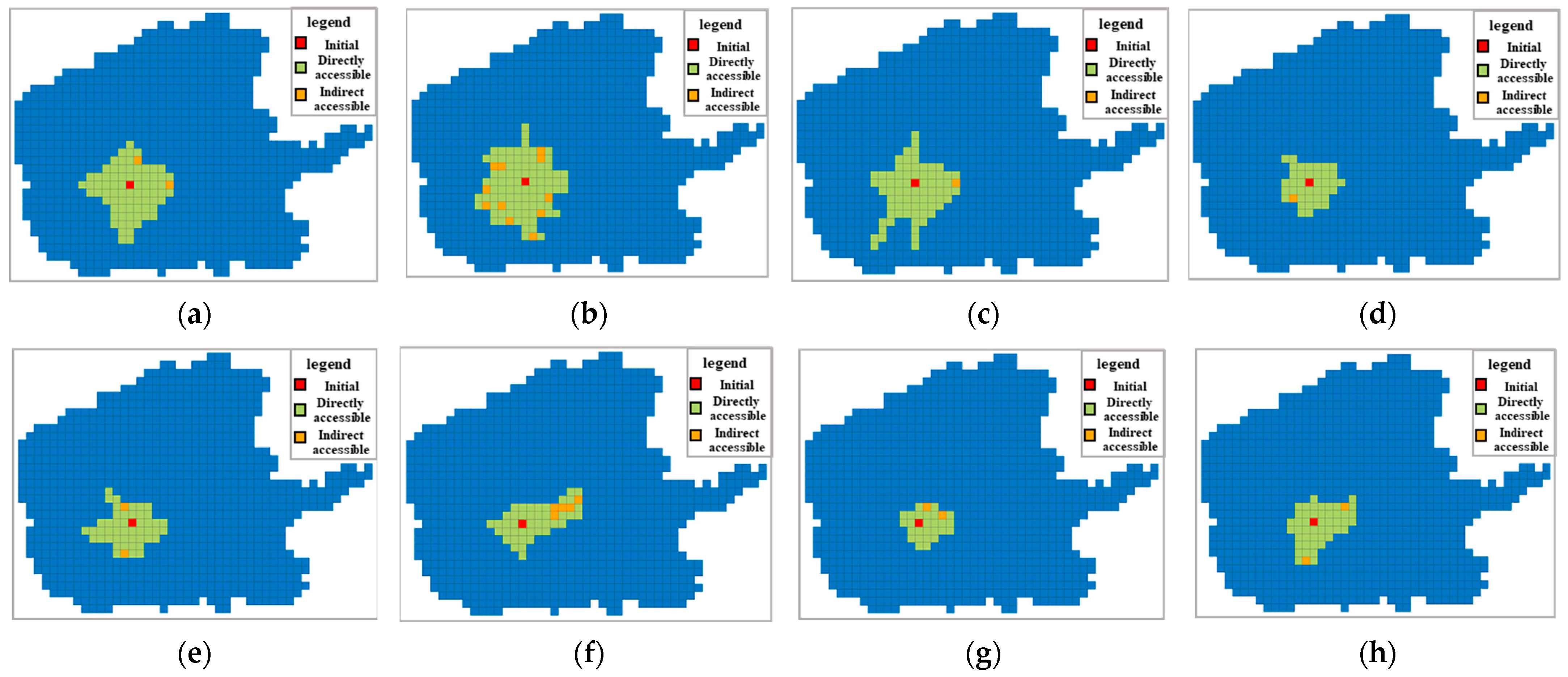
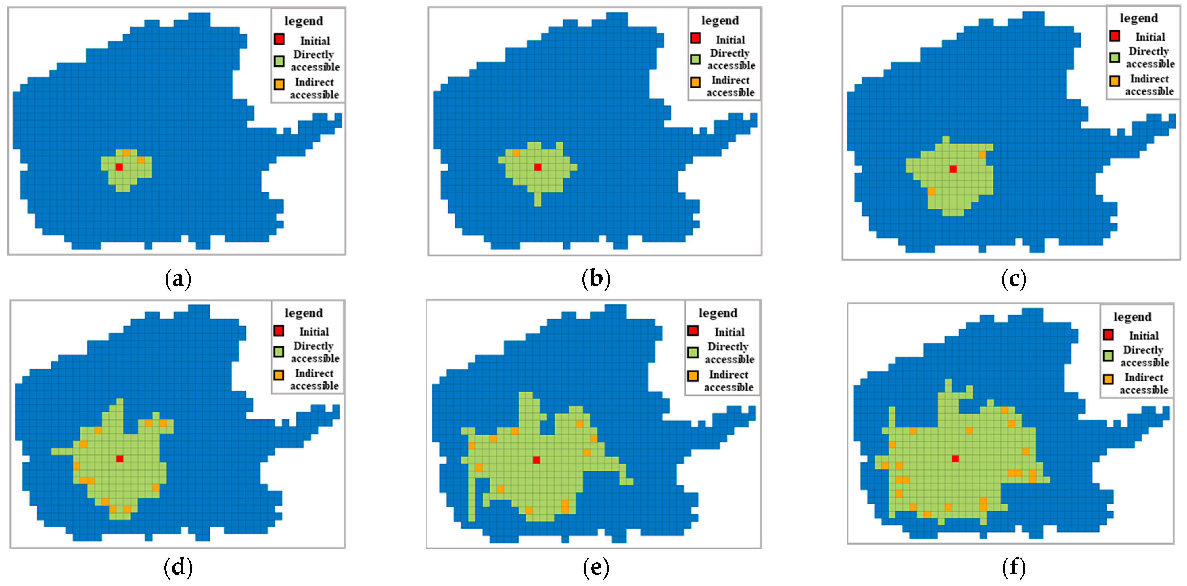
4.1.1. Real-Time Accessible Range Analysis

(1)
Accessible Range of Different Periods at the Same Time Interval
To analyze the time-varying law of the accessible range of taxis in a day, grid 330 is used as the starting grid, and the time interval is 10 min. Taking November 8 as an example, the time-varying map of the accessible range of a total of eight periods in a day is obtained, as shown in Figure 9. It can be seen from Figure 9 that the three periods of 00:00–00:10, 03:00–03:10, and 06:00–06:10 have the largest accessible range. This is because there are fewer vehicles on the road from midnight to early morning, the average speed of the driver is higher, and the probability of encountering a traffic jam is lower so the taxi can drive to a farther area in ten minutes. Relatively speaking, the accessible range of 09:00–09:10 and 18:00–18:10 is the smallest, which is only one-third of the accessible range at midnight. These two periods are also the morning and evening peaks of traffic, and there are a large number of vehicles on the road, which leads to taxis that can only travel closer in ten minutes.
(2)
Accessible Range of the Same Period at Different Time Intervals
The setting of the time interval also has a very significant impact on the accessible range rationality. Grid 330 is selected as the starting point, and the starting time point is 18:00, and the time interval is increased in turn to compare the changes in the accessible range. Figure 10 shows the accessible range of time intervals of 10 min, 20 min, 30 min, 40 min, 50 min, and 1 h. It can be seen that the accessible range increases significantly with the increase in the time interval. Specifically, the accessible range contains 29 grids when the time interval is 10 min, and when the time interval is set to 1 h, the accessible range contains more than 300 grids, which is ten times the time interval of 10 min. Therefore, it is necessary to select a reasonable time interval when recommending passenger hotspots to taxi drivers seeking passengers.
In summary, the accessible range of different periods at the same time interval in a day and the same period at different time intervals in a day is dynamically changing in real-time. Compared with the previous methods such as delineating the accessible range with a given fixed radius, this study considers that the accessible range will change with factors such as road traffic conditions in different periods when formulating the optimal scheduling area method of taxis [33,34]. That is, the dynamic scheduling area is recommended to taxi drivers in real-time, which is more in line with the travel characteristics of taxis.

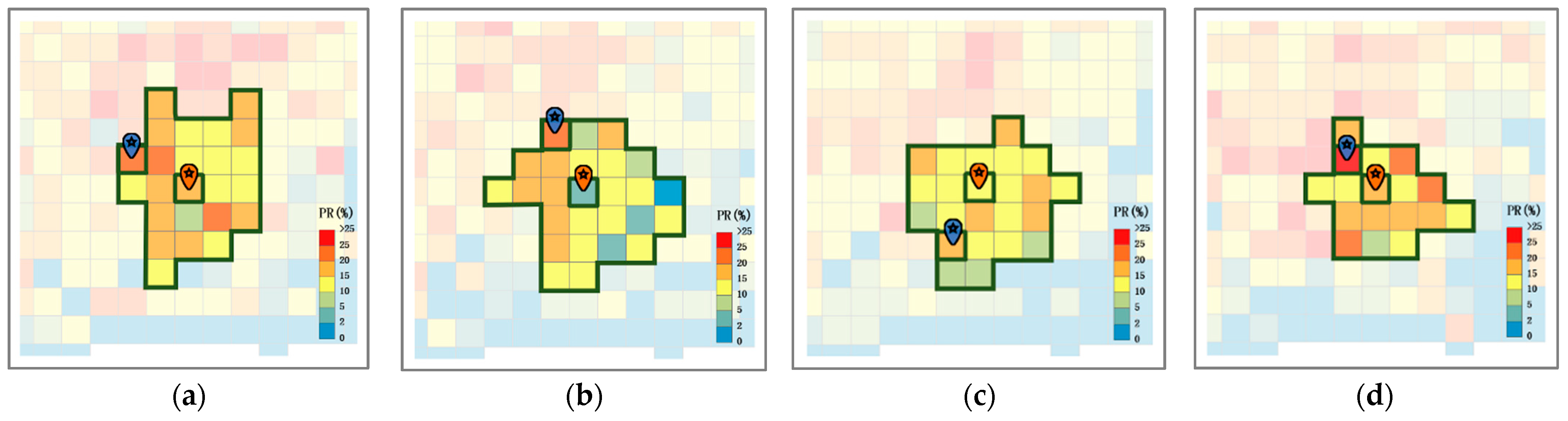
4.1.2. Dynamic Identification of Optimal Cruising Area Based on Real-Time Pick-Up Ratio

Based on the real-time optimal cruising area identification method, this study discusses the changes in the optimal cruising area obtained under different periods at the same time interval and the same period at different time intervals from the same initial grid, to verify the advancement, rationality, and effectiveness of the real-time cruising area identification method.
(1)
Identification of Optimal Cruising Area in Different Time Periods on the Same Date
To analyze the time-varying law of taxi passenger hotspots in a day, the taxi GPS trajectory data on November 8 (Friday) were selected. Grid 330 was used as the starting point, and the time interval was ten minutes. The taxi grid pick-up ratio in the eight time periods of 0:00–0:10, 3:00–3:10, 6:00–6:10, 9:00–9:10, 12:00–12:10, 15:00–15:10, 18:00–18:10, and 21:00–21:10 within a day was calculated, and the optimal cruising area of the taxi in each period was identified. The results are shown in Figure 11. The grid color in Figure 11 represents the value of the pick-up ratio (PR). The red grid has the largest PR value and the blue grid has the smallest PR value. The area enclosed by the dark green solid line in the figure is the reachable range under the corresponding conditions. The orange marker is located at the initial grid 330, and the blue marker represents the optimal cruising area identified by the model.
From Figure 11, it can be seen that the taxi accessible range boundary and the real-time pick-up ratio from the initial grid, grid 330, are different in different periods, and the pick-up ratio of the optimal cruising area is effectively improved compared with the initial grid. On the whole, the model can effectively improve the pick-up ratio passenger probability of taxis in each period. The absolute value of the grid pick-up ratio increased by 19.1% on average, with a year-on-year increase of 288.7%. Specifically, in the three time periods of 9:00–9:10, 12:00–12:10, and 15:00–15:10, the increase in the pick-up ratio is relatively low, at 127.0%; in the three time periods of 0:00–0:10, 3:00–3:10, and 6:00–6:10, the pick-up ratio increased by 466.0%, which was more than three times that of the former. The above findings are consistent with the characteristics of residents’ travel; that is, residents’ demand for taxi travel is relatively average during the day, and drivers are more likely to pick up passengers in various regions of the city [35]. However, from midnight to early morning, different from traditional modes of transportation such as public transportation and the subway, the demand for taxi travel is still relatively strong, but the distribution of travel is no longer scattered, and it is concentrated in nightlife-rich areas such as an urban central business district [36]. It can be seen that the model constructed in this study can accurately identify short-term regional hotspots, which greatly improves the probability of picking up passengers.
(2)
Identification of Optimal Cruising Area in the Same Period on Different Dates
To analyze the change in passenger hotspots and the model applicability in the same grid in the same period on different dates, this study took grid 330 as the starting point and 19:00–19:10 as the study period, and identified the optimal cruising search area of taxis from 5–8 November. The results are shown in Figure 12. The interpretation of color and mark in Figure 12 is the same as in Figure 11.
From Figure 12, it can be seen that the accessible range and pick-up ratio of taxis in the same period on different dates are still dynamic, reflecting the time-varying law of taxi travel demand hotspots. On 5 November, 6 November, 7 November, and 8 November, at 19:00–19:10, the pick-up ratio of the initial grid, grid 330, was 15.1%, 4.95%, 11.3%, and 15.4%, respectively. According to the model, the maximum pick-up ratio areas were identified as grid 298 (pick-up ratio of 24.7%), grid 327 (pick-up ratio of 20.0%), grid 323 (pick-up ratio of 19.9 %), grid 326 (pick-up ratio of 26.4%). The pick-up ratio increased by 63.6%, 304%, 76.1%, 71.4%. It can be seen that the increase in the pick-up ratio on different dates is similar, and the increase in the pick-up ratio on Saturday is higher. This may be due to the increase in people’s travel for entertainment and other activities on Saturday, which leads to an increase in travel demand. Therefore, it is not proper to distinguish between working days and rest days to predict the residents’ travel hotspots and cruising scheduling in the taxi cruising search demand analysis. The model constructed in this study has real-time performance [37], which can dynamically adjust the recommendation area according to the actual situation, and has more reference value for taxi drivers with immediate needs.
Through the analysis of the above two levels of different periods on the same date and the same period on different dates, compared with the traditional research, the taxi real-time optimal cruising passenger search area model constructed in this study is reasonable and effective and has certain practicability and advancement. On the one hand, the model can effectively identify the optimal cruising area, and the pick-up ratio of the area is greatly improved compared with the initial position of the driver; on the other hand, the constructed model is not limited in time and space and can provide real-time personalized needs for taxi drivers in the study area, that is, the real-time dynamic identification of cruising areas based on travel demand hotspots.

4.2. Real-Time Dynamic Prediction of Optimal Cruising Area

This study took taxi drivers within grid 382 as an example and predicted the dynamic accessible range and real-time optimal scheduling area of taxis based on the deep learning algorithm. The study area is located in Qujiang Dayue City and the Big Wild Goose Pagoda area of Xi’an (as shown in Figure 13), and the surrounding land use is mainly tourism and commerce. During the daytime, the travel demand in this area is relatively large, while at midnight, the corresponding scenic spots and shopping malls are non-operating. The taxi travel demand in this area is relatively small, which belongs to the relative demand depression. Compared with the daytime, the probability of taxis receiving passengers in this area during the midnight period is relatively small. Therefore, this study took the no-load taxi from 0:00 to 0:10 on 30 November (Saturday) as an example to verify the effectiveness of the UTCN accessible range prediction model and the MTCN pick-up ratio prediction model, and further identify the optimal taxi scheduling area based on the pick-up ratio prediction.

4.2.1. Real-Time Accessible Range Prediction

Taking grid 382 as the study area, the taxi travel data from 1–29 November were selected, and 4176 sets of time series data sets of the accessible range were obtained at a time interval of 10 min. There are 945 grid values every 10 min, and the grid value is 0/1/2/3, which represents an inaccessible range, a direct accessible range, indirect accessible range I, and indirect accessible range II, respectively. Based on the real-time accessible range measurement model, the accessible state value of the whole day on November 30 was predicted.
(1)
Experimental Setting and Evaluation Index Selection
In this study, the grid search method [38] is used to verify the UTCN model, and the model training effect is the best when the convolution kernel size is 3. The parameter values are as follows: the expansion factor is set to 2, the training window size is 144, the number of convolution kernels is 128, the dropout is set to 0.2, the learning rate is 0.001, the parameters are updated using the Adam optimizer and mean squared error (MSE) loss function, and the number of network training cycles is set to 500. Simultaneously, RNN (using the loop structure to share parameters at each time step of the sequence, which can take into account the time dependence), GRU (introducing update gate and reset gate to solve the gradient problem of traditional RNN, selectively retaining the control information of the update gate, and selectively ignoring the control information of the reset gate), LSTM (introducing the mechanism of input gate, forgetting gate, and output gate to input the long-term and short-term memory network structure), and other models were selected as benchmark models for model comparison and verification. Meanwhile, this study mainly selected the mean absolute error (MAE), root mean square error (RMSE), and mean absolute percentage error (MAPE) to measure the prediction effect of different models.
(2)
Analysis of Accessible Range Prediction Results
Based on the benchmark model, the performance evaluation indexes of different models were obtained, as shown in Table 3.
From Table 3, the MAE value of the UTCN model was reduced by 54.162%, 37.136%, and 22.589%, respectively, compared with the RNN, LSTM, and GRU models. The RMSE was reduced by 29.199%, 19.611%, and 10.329%, respectively, and the MAPE value was reduced by 7.709%, 5.069%, and 1.467%, respectively. It can be seen that the TCN model preserves the convolution internal structure of the original CNN model, gets rid of the long-term dependence of the traditional RNN, and improves the problem that the size of the original CNN convolution kernel is limited. That is, the convolution kernels of different sizes are used to convolve the time series. Compared with Recurrent Neural Networks such as LSTM and GRU, the number of parameters is relatively small, which can be calculated efficiently in parallel, making the model prediction results more accurate.
Therefore, taking 00:00–00:10 on 30 November as an example, the accessible range diagram is similar to the range diagram predicted using the UTCN model, as shown in Figure 14.

4.2.2. Importance Analysis of Variables Related to Pick-Up Ratio

With an interval of 10 min, the day was divided into 144 time periods. The 15 indicators to be screened in Section 3.2.3 were used as input variables, and the pick-up ratio was used as an output variable, which is imported into the GBDT model to analyze the importance of variable characteristics. The data from Monday to Wednesday were used as the training set, and the data from Thursday and Friday were used as the test set. The model fitting and prediction were carried out to obtain the importance of each input feature for the whole prediction result, that is, the pick-up ratio. The influence degree values of each variable obtained through operation are as follows: “CR” = 5612, “VD” = 5606, “HP” = 4937, “APR” = 4222, “AOS” = 3285, “DR” = 3092, “H” = 2543, “LPR” = 2180, “AQI” = 1334, “WS” = 1159, “AT” = 1059, “HD” = 742, “M” = 577, “WC” = 326, “D” = 316.
A radar map was drawn to visually display the above results, as shown in Figure 15. It can be seen that the influence degree of each spatial and temporal characteristic on the pick-up ratio is ranked. The farther the index value is from the center of the circle, the more important the variable characteristics are. Compared with the characteristic indexes of the cruising ratio (CR), vehicle density (VD), heat of pick-up (HP), adjacent pick-up ratio (APR), average operating speed (AOS), drop-off ratio (DR), hour (H), last pick-up ratio (LPR), and air quality index (AQI), the influence degree of the weather condition (WC) and day (D) is very low. Therefore, before the prediction of the pick-up ratio, it is necessary to eliminate the indicators with low correlation and retain the indicators significantly related to them, to improve the accuracy of the prediction model.

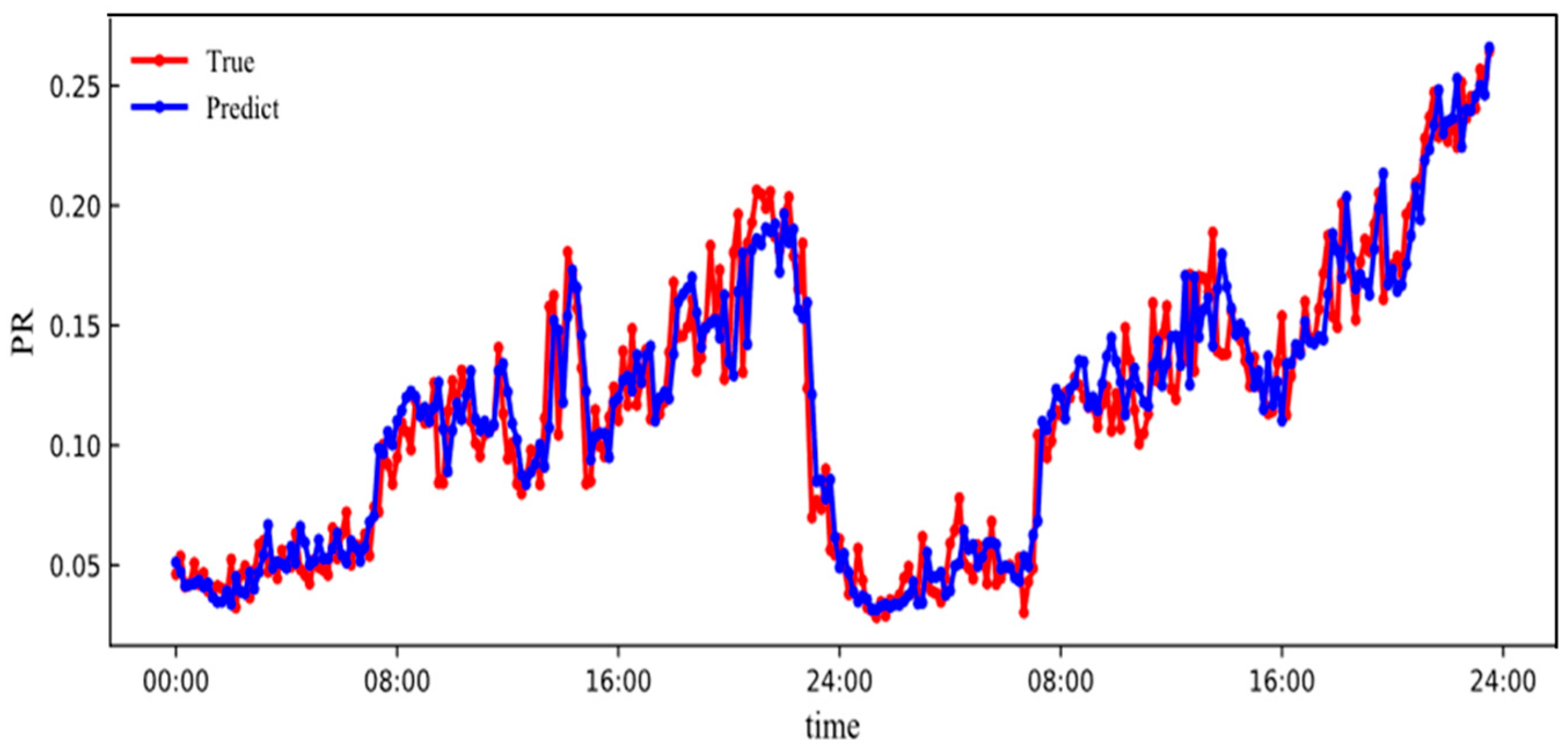
4.2.3. Real-Time Pick-Up Ratio Prediction

(1)
Experimental Setting and Evaluation Index Selection
Taking grid 382 as an example, the taxi travel data from 1–29 November were selected, and the time series set was composed of the above input variables of 10 min. The data of the previous 22 days were used as the training set, and the data of the next 7 days were used as the test set to predict the pick-up ratio. In the MTCN network, the expansion factor was set to 2, the training window size was 144, the convolution kernel size was set to 3, the dropout was set to 0.2, the learning rate was 0.001, and the number of iterations was 1000. The Adam optimizer and MSE loss function were used to update the parameters. RNN, GRU, LSTM, and MTCN were still selected for the comparison model, and MAE, RMSE, and MAPE were selected for model performance evaluation.
(2)
Identification of the Optimal Scheduling Area under the Prediction of Pick-up Ratio
Based on the comparison of the benchmark model, the performance evaluation indexes of different pick-up ratio prediction models were obtained, as shown in Table 4.
It can be seen from Table 4 that when predicting the pick-up ratio, the MAE value of the MTCN model is 60.345%, 32.353%, and 20.69% lower than that of the RNN, LSTM, and GRU models, respectively. The RMSE was reduced by 22.449%, 10.938%, and 4.202%, respectively, and the MAPE value was reduced by 20.613%, 15.438%, and 1.4349%, respectively. Thus, the MTCN model was more accurate in predicting the pick-up ratio based on multivariate prediction. Therefore, taking grid 330 as an example, based on the MTCN model, the fitting results of the predicted value and the actual value of the pick-up ratio of the whole day (at 10 min intervals) on 30 November were compared, as shown in Figure 16. Among them, the blue line is the true value, the red line is the predicted value, and the MAE, RMSE, and MAPE of the predicted value and the actual value are 0.023, 0.027, and 7.329%, respectively. It can be seen that the model accuracy is high. Based on this, the predicted pick-up ratio of 00:00–00:10 on Saturday, 30 November is 24.69%.
Based on the pick-up ratio of each grid in the accessible range, it is identified that the optimal scheduling area with grid 382 as the initial grid on 30 November is grid 327 (the grid indicated by the arrow in Figure 17). The pick-up ratio is 30.0%, which is much higher than 12.1% of the initial grid, and higher than all other grids in the region. Therefore, taking grid 327 as the taxi cruising endpoint, compared with the initial grid, grid 382, the pick-up ratio of the optimal cruising grid, grid 327, identified using the model is increased by 17.9%, and the probability of receiving passengers is increased by 148.0% year on year.

5. Conclusions

From the timeliness, accessibility, and dynamics of taxi cruising area identification and recommendation, this study proposed a dynamic identification strategy of taxi optimal cruising areas based on spatio-temporal data. The main conclusions are as follows:
This study proposed a real-time accessible range prediction model of taxis based on GCOM. The concept of the cumulative opportunity method was combined with the accessible range of the road network, and the concept of grid compensation was proposed, which fills the influence of insufficient GPS trajectory data or low grid demand regarding near inaccessible and far accessible areas. Then, the UTCN algorithm was proposed to obtain the real-time dynamic accessible range of taxis. The results show that the accessible range of the same grid under different time intervals changes with time, indicating the time variability of the accessible range. Compared with the traditional research methods that mostly use static indicators to predict travel hotspots in morning and evening peaks, the spatio-temporal data chain is constructed in minutes, which can realize the real-time effectiveness of taxi-seeking passenger area identification and recommendation. Based on the actual situation of the road network, this study predicts the accessible range of taxis in a fixed period in real-time, making the recommended area more implementable.
Then, this study analyzed the factors affecting the cruising mode of taxi drivers from four aspects, traffic attributes, time periodicity, spatial attributes, and external environmental attributes, built a GBDT framework, and screened out the characteristic variables with high correlation with the output variable pick-up ratio. The MTCN algorithm was constructed to predict the future pick-up ratio value of each grid, and the real-time passenger pick-up level of the whole study area was evaluated accordingly. The area with the highest pick-up ratio in the accessible range in different periods was identified as the optimal cruising area. The study found that the optimal cruising area pick-up ratio of taxis in different periods of the same date and the same period of different dates had been greatly improved compared with the initial pick-up ratio, with an average increase of 19.1% and 11.1%, respectively, and the total year-on-year increase had reached 288.7% and 63%. The results show that the model can dynamically identify the cruising area in real-time and greatly improve the regional pick-up ratio, thus providing a basis for reducing the empty driving rate of taxi travel. The study conclusion can effectively improve the efficiency of taxi cruising and lay a foundation for the optimal cruising route decision, to provide a scientific basis for formulating the corresponding taxi management strategy.
In summary, this study defined the area with the highest pick-up ratio in different periods as the optimal cruising area, which can improve the probability of taxis receiving passengers, avoid aimless cruising, and reduce the cruising distance of taxis to a certain extent. At the same time, from the perspective of passengers, it solves the shortage of taxis in hotspots, thus shortening the waiting time of passengers. Finally, based on the comparative analysis of models, the UTCN algorithm and the MTCN algorithm have the highest prediction accuracy. On the one hand, it is verified that the predicted accessible range is similar to the actual accessible range. On the other hand, the pick-up ratio of the optimal cruising area of taxis starting from different grid areas in different periods is significantly improved compared with the original area. That is, the reliability of the deep learning algorithm used in this study is verified from the model level.
Based on the optimal cruising area identification, the top three areas with the highest pick-up ratio can be recommended as alternative cruising areas for taxis in future research. Starting from the three aspects of taxi passenger cost-effectiveness, passenger travel efficiency cost-effectiveness, and environmental cost-effectiveness (carbon emissions), picking up the passenger path with the smallest total cost-effectiveness and the corresponding alternative cruising area are recommended to the no-load taxi driver. That is, while solving the problem of unbalanced supply and demand of taxi hotspots and shortening the empty driving distance, the total cost of the no-load taxi to pick up passengers is considered. Therefore, the above analysis can shorten the empty driving distance of taxis during operation, improve the efficiency of road cruising, reduce passenger waiting time, effectively reduce the waste of taxi resources, further alleviate traffic congestion and environmental pollution, and promote the sustainable development of urban traffic.

Author Contributions

Conceptualization, S.W. and J.W.; methodology, S.W., J.W. and D.L.; software, S.W.; validation, S.W., J.W. and C.M.; formal analysis, S.W. and D.L.; writing—original draft preparation, S.W. and J.W.; writing—review and editing, S.W., J.W. and L.C.; visualization, C.M. and D.L.; supervision, L.C.; funding acquisition, J.W. All authors have read and agreed to the published version of the manuscript.

Funding

This research was funded by the National Natural Science Foundation of China (Grant no. 52272316) and the Natural Science Basic Research Program of Shaanxi, China (No. 2023JC-YB-332).

Institutional Review Board Statement

Not applicable.

Informed Consent Statement

Not applicable.

Data Availability Statement

Some or all data, or models, that support the findings of this study are available from the corresponding author upon reasonable request.

Conflicts of Interest

The authors declare no conflicts of interest.

References

  1. Shi, K.; Shao, R.; De Vos, J.; Cheng, L.; Witlox, F. The Influence of Ride-Hailing on Travel Frequency and Mode Choice. Transp. Res. Part D Transp. Environ. 2021, 101, 103125. [Google Scholar] [CrossRef]
  2. Di, W.; Tomio, M.; Morikawa, T. Interrelationships between Traditional Taxi Services and Online Ride-Hailing: Empirical Evidence from Xiamen, China. Sustain. Cities Soc. 2022, 83, 103924. [Google Scholar]
  3. Taxi Management Office of Xi’an and Chang’an University. Available online: http://m.xinhuanet.com/sn/2021-02/20/c_1127117639.htm (accessed on 20 October 2023).
  4. Zheng, L.; Xia, D.; Zhao, X.; Tan, L.; Li, H.; Chen, L.; Liu, W. Spatial-Temporal Travel Pattern Mining Using Massive Taxi Trajectory Data. Phys. A 2018, 501, 24–41. [Google Scholar] [CrossRef]
  5. Qu, B.; Yang, W.; Cui, G.; Wang, X. Profitable Taxi Travel Route Recommendation based on Big Taxi Trajectory Data. IEEE Trans. Intell. Transp. Syst. 2020, 21, 653–668. [Google Scholar] [CrossRef]
  6. Sung, H.; Choi, K.; Lee, S.; Cheon, S. Exploring the Impacts of Land Use by Service Coverage and Station-Level accessibility on Rail Transit Ridership. J. Transp. Geogr. 2014, 36, 134–140. [Google Scholar] [CrossRef]
  7. Zhang, W.; Zhao, Y.; Cao, X.J.; Lu, D.; Chai, Y. Nonlinear Effect of Accessibility on Car Ownership in Beijing: Pedestrian-Scale Neighborhood Planning. Transp. Res. D Transp. Environ. 2020, 86, 102445. [Google Scholar] [CrossRef]
  8. Zhao, K.; Khryashchev, D.; Vo, H. Predicting Taxi and Uber Demand in Cities: Approaching the Limit of Predictability. IEEE Trans. Knowl. Data Eng. 2021, 33, 2723–2736. [Google Scholar] [CrossRef]
  9. Lyu, T.; Wang, Y.; Ji, S.; Feng, T.; Wu, Z. A multiscale spatial analysis of taxi ridership. J. Transp. Geogr. 2022, 113, 103718. [Google Scholar] [CrossRef]
  10. Wang, Z.; Zhang, Y.; Jia, B.; Gao, Z. Comparative Analysis of Usage Patterns and Underlying Determinants for Ride-hailing and Traditional Taxi Services: A Chicago Case Study. Transport. Res. Part A Policy Pract. 2023, 179, 103912. [Google Scholar] [CrossRef]
  11. Su, R.; Fang, Z.; Luo, N.; Zhu, J. Understanding the Dynamics of the Pick-Up and Drop-Off Locations of Taxicabs in the Context of a Subsidy War among E-Hailing Apps. Sustainability 2018, 10, 1256. [Google Scholar] [CrossRef]
  12. Shen, H.; Zou, B.; Lin, J.; Liu, P. Modeling Travel Mode Choice of Young People with Differentiated E-hailing Ride Services in Nanjing China. Transp. Res. Part D Transp. Environ. 2020, 78, 102216. [Google Scholar] [CrossRef]
  13. Demissie, M.G.; Kattan, L.; Phithakkitnukoon, S.; De Almeida Correia, G.H.; Veloso, M.L.; Bento, C. Modeling Location Choice of Taxi Drivers for Passenger Pickup Using GPS Data. IEEE Trans. Intell. Transp. Syst. Mag. 2020, 13, 70–90. [Google Scholar] [CrossRef]
  14. Kelobonye, K.; Zhou, H.; McCarney, G.; Xia, J.C. Measuring the Accessibility and Spatial Equity of Urban Services under Competition Using the Cumulative Opportunities Measure. J. Transp. Geogr. 2020, 85, 102706. [Google Scholar] [CrossRef]
  15. Wong, R.; Szeto, W.Y.; Wong, S.C. A Cell-Based Logit-Opportunity Taxi Customer-Search Model. Transp. Res. Part C Emerg. Technol. 2014, 48, 84–96. [Google Scholar] [CrossRef]
  16. Chen, F.; Yin, Z.; Ye, Y.; Sun, D. Taxi Hailing Choice Behavior and Economic Benefit Analysis of Emission Reduction based on Multi-Mode Travel Big Data. Transp. Policy 2020, 97, 73–84. [Google Scholar] [CrossRef]
  17. Szeto, W.Y.; Wong, R.C.P.; Yang, W.H. Guiding Vacant Taxi Drivers to Demand Locations by Taxi-Calling Signals: A Sequential Binary Logistic Regression Modeling Approach and Policy Implications. Transp. Policy 2019, 76, 100–110. [Google Scholar] [CrossRef]
  18. Hochreiter, S.; Schmidhuber, J. Long Short-term Memory. Neural Comput. 1997, 9, 1735–1780. [Google Scholar] [CrossRef]
  19. Lv, M.; Hong, Z.; Chen, L.; Chen, T.; Zhu, T.; Ji, S. Temporal Multi-Graph Convolutional Network for Traffic Flow Prediction. IEEE Trans. Intell. Transp. Syst. 2021, 22, 3337–3348. [Google Scholar] [CrossRef]
  20. Wang, H.; Zhang, R.; Cheng, X.; Yang, L. Hierarchical Traffic Flow Prediction based on Spatial-Temporal Graph Convolutional Network. IEEE Trans. Intell. Transp. Syst. 2022, 23, 16137–16147. [Google Scholar] [CrossRef]
  21. Zhan, X.; Qian, X.; Ukkusuri, S.V. A Graph-Based Approach to Measuring the Efficiency of an Urban Taxi Service System. IEEE Trans. Intell. Transp. Syst. 2016, 17, 2479–2489. [Google Scholar] [CrossRef]
  22. Li, Q.; Cheng, R.; Ge, H. Short-Term Travel Demand Prediction of Online Ride-Hailing Based on Multi-Factor GRU Model. Phys. A 2023, 610, 128410. [Google Scholar] [CrossRef]
  23. Chang, W.; Chen, X.; He, Z.; Zhou, S. A Prediction Hybrid Framework for Air Quality Integrated with W-BiLSTM(PSO)-GRU and XGBoost Methods. Sustainability 2023, 15, 16064. [Google Scholar] [CrossRef]
  24. Yan, J.; Mu, L.; Wang, L.; Ranjan, R.; Zomaya, A.Y. Temporal Convolutional Networks for the Advance Prediction of ENSO. Sci. Rep. 2020, 10, 650705. [Google Scholar] [CrossRef] [PubMed]
  25. Luo, A.; Shangguan, B.; Yang, C.; Gao, F.; Fang, Z.; Yu, D. Spatial-Temporal Diffusion Convolutional Network: A Novel Framework for Taxi Demand Forecasting. ISPRS Int. J. Geo-Inf. 2022, 11, 193. [Google Scholar] [CrossRef]
  26. Wang, S.; Wang, J.; Li, W.; Fan, J.; Liu, M. Revealing the Influence Mechanism of Urban Built Environment on Online Car-Hailing Travel Considering Orientation Entropy of Street Network. Discret. Dyn. Nat. Soc. 2022, 2022, 3888800. [Google Scholar] [CrossRef]
  27. Bi, H.; Ye, Z. Exploring Ridesourcing Trip Patterns by Fusing Multi-Source Data: A Big Data Approach. Sustain. Cities Soc. 2021, 64, 102499. [Google Scholar] [CrossRef]
  28. Cao, Y.; Liu, L.; Dong, Y. Convolutional Long Short-Term Memory Two-Dimensional Bidirectional Graph Convolutional Network for Taxi Demand Prediction. Sustainability 2023, 15, 7903. [Google Scholar] [CrossRef]
  29. Lai, Y.; Lv, Z.; Li, K.C.; Liao, M. Urban Traffic Coulomb’s Law: A New Approach for Taxi Route Recommendation. IEEE Trans. Intell. Transp. Syst. 2019, 20, 3024–3037. [Google Scholar] [CrossRef]
  30. Zhang, T.; Huang, Y.; Liao, H.; Liang, Y. A Hybrid Electric Vehicle Load Classification and Forecasting Approach based on GBDT Algorithm and Temporal Convolutional Network. Appl. Energy 2023, 351, 121768. [Google Scholar] [CrossRef]
  31. Liu, K.; Chen, J.; Li, R.; Peng, T.; Ji, K.; Gao, Y. Nonlinear Effects of Community Built Environment on Car Usage Behavior: A Machine Learning Approach. Sustainability 2022, 14, 6722. [Google Scholar] [CrossRef]
  32. Chen, J.; Li, W.; Zhang, H.; Jiang, W.; Li, W.; Sui, Y.; Song, X.; Shibasaki, R. Mining Urban Sustainable Performance: GPS Data-based Spatio-Temporal Analysis on on-Road Braking Emission. J. Clean. Prod. 2020, 270, 122489. [Google Scholar] [CrossRef]
  33. Bian, R.R.; Wilmot, C.G.; Wang, L. Estimating Spatio-temporal Variations of Taxi Ridership Caused by Hurricanes Irene and Sandy: A Case Study of New York City. Transp. Res. Part D Transp. Environ. 2019, 77, 627–638. [Google Scholar] [CrossRef]
  34. Kim, H.; Lee, K.; Park, J.S.; Song, Y. Transit Network Expansion and Accessibility Implications: A Case Study of Gwangju Metropolitan Area, South Korea. Res. Transp. Econ. 2018, 69, 544–553. [Google Scholar] [CrossRef]
  35. Jiao, W.; Huang, W.; Fan, H. Evaluating Spatial Accessibility to Healthcare Services from the Lens of Emergency Hospital Visits based on Floating Car Data. Int. J. Digit. Earth 2022, 15, 108–133. [Google Scholar] [CrossRef]
  36. Li, B.; Cai, Z.; Jiang, L.; Su, S.; Huang, X. Exploring Urban Taxi Ridership and Local Associated Factors Using GPS Data and Geographically Weighted Regression. Cities 2019, 87, 68–86. [Google Scholar] [CrossRef]
  37. Gonzales, E.J.; Yang, C.; Morgul, E.F.; Ozbay, K. Modeling Taxi Demand with GPS Data from Taxis and Transit; Technical Representative CA-MNTRC-14-1141; Mineta National Transit Research Consortium: New York, NY, USA, 2014. [Google Scholar]
  38. Sun, Y.; Ding, S.; Zhang, Z. An Improved Grid Search Algorithm to Optimize SVR for Prediction. Soft Comput. 2021, 25, 5633–5644. [Google Scholar] [CrossRef]
Figure 1. Study area and grid division.
Sustainability 16 00866 g001
Figure 2. Example of identification for pick-up and drop-off location.
Sustainability 16 00866 g002
Figure 3. Grid accumulation diagram. (a) The actual path through the grid range. (b) Grid cumulative accessible range.
Sustainability 16 00866 g003
Figure 4. Schematic diagram of atrous convolution.
Sustainability 16 00866 g004
Figure 5. Schematic diagram of residual module.
Sustainability 16 00866 g005
Figure 6. Flow chart of UTCN accessible range prediction.
Sustainability 16 00866 g006
Figure 7. GBDT algorithm schematic diagram.
Sustainability 16 00866 g007
Figure 8. Real-time dynamic prediction flow chart of taxi optimal cruising area.
Sustainability 16 00866 g008
Figure 9. The accessible range of different periods at the same time interval in a day. (a) 00:00–00:10, (b) 03:00–03:10, (c) 06:00–06:10, (d) 09:00–09:10, (e) 12:00–12:10, (f) 15:00–15:10, (g) 18:00–18:10, (h) 21:00–21:10.
Sustainability 16 00866 g009
Figure 10. The accessible range of the same period at different time intervals in a day. (a) 18:00–18:10, (b) 18:00–18:20, (c) 18:20–18:30, (d) 18:00–18:40, (e) 18:00–18:50, (f) 18:00–19:00.
Sustainability 16 00866 g010
Figure 11. Optimal cruising area in different periods on the same date. (a) 0:00–0:10, (b) 3:00–3:10, (c) 6:00–6:10, (d) 9:00–9:10, (e) 12:00–12:10, (f) 15:00–15:10, (g) 18:00–18:10, (h) 21:00–21:10.
Sustainability 16 00866 g011
Figure 12. Optimal cruising area in the same period on the different dates; (a) 5 November, (b) 6 November, (c) 7 November, (d) 8 November.
Sustainability 16 00866 g012
Figure 13. Study area diagram.
Sustainability 16 00866 g013
Figure 14. Dynamic forecast results of available range from 00:00 to 00:10 on 30 November.
Sustainability 16 00866 g014
Figure 15. Radar chart of index characteristic importance.
Sustainability 16 00866 g015
Figure 16. Prediction results of grid 382 pick-up ratio (00:00–00:10 on 30 November).
Sustainability 16 00866 g016
Figure 17. Identification of optimal cruising area during 00:00–00:10 on 30 November.
Sustainability 16 00866 g017
Table 1. Examples of spatio-temporal data fields.
Data FieldMeaning Data Example 1Data Example 2
LPNLicense plate numberA****00A****34
TSTimestamp1,573,261,2751,573,261,305
C_wgsCoordinatePOINT [108.925200, 34.347733]POINT [108.925167, 34.350217]
SpeedSpeed1232
Car_statCarrying state11
IH_stIdle or hired status00
IDGrid_id285285
POIPoints of interest307307
WCWeather conditionsSunnyCloudy
ATApparent temperature8.34.8
WSWind speed3.14.5
AQIAir quality index4974
Table 2. Traffic Attribute Variables.
VariableNotationFormula
Pick-up ratio
(PR)
The probability of all cruising taxis in grid i picking up passengers within a certain period, [t1, t2). P R i , t 1 , t 2 = t 1 t 2 P i t 1 t 2 N C i , t 1 t 2 N C i > 0 0 , t 1 t 2 N C i = 0
Drop-off ratio
(DR)
The probability of dropping off all passengers from operating taxis in grid i within a certain period, [t1, t2). D R i , t 1 , t 2 = t 1 t 2 D i t 1 t 2 N O i , t 1 t 2 N O i > 0 0 , t 1 t 2 N O i = 0
Cruising ratio
(CR)
The number of all idle cruising taxis in grid i accounts for the proportion of the total number of taxis in the grid within a certain period, [t1, t2). C R i , t 1 , t 2 = t 1 t 2 N C i t 1 t 2 N i , t 1 t 2 N i > 0 0 , t 1 t 2 N i = 0
Heat of pick-up
(HP)
The number of all cruising taxis picking up passengers in grid i within a certain period, [t1, t2). H P i , t 1 , t 2 = t 1 t 2 P i
Heat of drop-off
(HD)
The number of all hiring taxis dropping off passengers in grid i within a certain period, [t1, t2). H D i , t 1 , t 2 = t 1 t 2 D i
Vehicle density
(VD)
The number of operating taxis per unit area. V D i , t 1 , t 2 = t 1 t 2 N i A i
Average operation speed
(AOS)
The average speed of all hiring taxis in grid i is within a certain period, [t1, t2), which can effectively reflect the real-time congestion situation of the road. A O S i , t 1 , t 2 = t 1 t 2 j = 1 N O i V j N O i
Table 3. Comparison results of accessible range indexes of each model.
Evaluating IndicatorRNNLSTMGRUUTCN
MAE0.6130.4470.3630.281
RMSE1.4741.2851.1521.033
MAPE (%)5.8245.6625.4555.375
Table 4. Comparison results of pick-up ratio prediction of each model.
Evaluating IndicatorRNNLSTMGRUMTCN
MAE0.0580.0340.0290.023
RMSE0.1470.1280.1190.027
MAPE (%)9.2328.6677.4367.329
Disclaimer/Publisher’s Note: The statements, opinions and data contained in all publications are solely those of the individual author(s) and contributor(s) and not of MDPI and/or the editor(s). MDPI and/or the editor(s) disclaim responsibility for any injury to people or property resulting from any ideas, methods, instructions or products referred to in the content.

