A Feasibility Assessment of Heat Energy Productivity of Geothermal Wells Converted from Oil/Gas Wells

Zhang, Peng; Guo, Boyun

doi:10.3390/su16020768

Open AccessArticle

A Feasibility Assessment of Heat Energy Productivity of Geothermal Wells Converted from Oil/Gas Wells

by

Peng Zhang

and

Boyun Guo

^*

Energy Institute of Louisiana, University of Louisiana at Lafayette, Lafayette, LA 70504, USA

^*

Author to whom correspondence should be addressed.

Sustainability 2024, 16(2), 768; https://doi.org/10.3390/su16020768

Submission received: 1 December 2023 / Revised: 10 January 2024 / Accepted: 10 January 2024 / Published: 16 January 2024

(This article belongs to the Special Issue Sustainable Use and Techniques of Geothermal Energy)

Download

Browse Figures

Versions Notes

Abstract

:

The mitigation of greenhouse gas emissions necessitates a shift from fossil fuel to environmentally friendly energy, such as geothermal energy. It is advantageous to retrofit end-of-life oil/gas wells for geothermal energy extraction. Prior to repurposing depleted wells into geothermal wells, it is imperative to conduct the heat-energy potential assessment. In this work, an analytical model was developed for this purpose. A case study was conducted using the model and the data from a well in North-west Louisiana for a feasibility assessment. A sensitivity study was performed with the model to identify major factors affecting well productivity. The result of the case study shows that reverse circulation is 35% more efficient than direct circulation for improving the heat-energy productivity of geothermal wells converted from oil/gas wells. The sensitivity analysis revealed that well productivity increases with higher injection rates and greater horizontal wellbore lengths. Additionally, well productivity rises in correspondence with reservoir temperature as well as the temperature of the injected water. However, well productivity decreases as the thermal conductivity of the tubing insulation increases. Counteracting this trend, well productivity increases with thicker tubing insulation layers. This study furnishes engineers with an easy-to-use tool for predicting the heat-energy deliverability of wells converted from end-of-life oil/gas wells.

Keywords:

geothermal wells; heat transfer; well productivity; assessment; mathematical modeling

1. Introduction

Many thousands of oil/gas wells in the world are approaching their end-of-life stage [1,2,3]. It is costly and wasteful to simply plug and abandon (P&A) them [4,5]. How to use these wells to improve economics is a big issue. Some of these wells produce fluids with elevated temperatures [6,7,8]. If we convert them to geothermal wells for power generation, how much energy can we expect to produce from these wells? This work answers the question after a prior assessment of the energy productivity of the converted wells.

Geothermal energy is found everywhere on the earth [9,10,11]. Figure 1 shows the distribution and grade of geothermal energy resources in the conterminous United States [12]. Although high-grade geothermal energy (>100 mW/m²) is found in volcanic settings such as Hawaii, the Rocky Mountain, and Yellowstone in the United States, these settings do not contain oil and natural gas. Middle-grade (60 mW/m² to 100 mW/m²) geothermal energy has been found and not used in the sedimentary Gulf Coast Basin where many wells have been drilled for oil and gas production [13,14].

The process of using the heat from oil wells to generate electricity power was demonstrated in North Dakota [15,16,17]. Novel power generation technologies have recently been developed through advances in well conversion in the middle-grade geothermal energy region [18]. Through the implementation of the Organic Rankine Cycle (ORC) method, the geothermal fluid is passed through the ORC unit, where a heat exchanger facilitates the transfer of thermal energy to an internal working fluid, resulting in vaporization due to the lower boiling point of the working fluid (e.g., pentafluoropropane has a boiling point of 15.3 °C) [19,20]. The vaporized working fluid undergoes expansion to drive a turbine, which subsequently operates a generator to produce electricity. The Climeon Heat Power 150 kW module can be optimized for low-grade heat resources (70–120 °C). The modular design of this system affords flexibility and scalability, with capacity extendable from 150 kW units to installations of several megawatts for larger power outputs [18]. A few abandoned oil wells were tested for generating power [21,22]. However, the potential for converting the end-of-life oil wells to geothermal wells in other regions, such as the Gulf Coast Basin, is not known, which demands a mathematical heat transfer model for technical assessment.

Li et al. [23] developed an analytical model to predict gas temperature during the drilling of wells. Liu and Shan [24] presented a numerical solution of the heat transfer problem in a gas production system. Fu et al. [25] presented an analytical approach for modeling the transfer of heat energy from a geothermal zone to a superjacent gas hydrate reservoir. A common limitation of these earlier models is the lack of consideration given to the effects of tubing insulation on heat transfer.

In all of the above-mentioned models, direct circulation of water is assumed, i.e., water is injected into the inside of the pipe/tubing and returned through the annulus to the surface. It is expected that direct circulation gives low efficiency of heat transfer from the pay zone to the surface due to the heat loss from the annulus to the surrounding formation rock along the flow path. This work presents a new analytical model for heat transfer in well systems with reverse circulation, i.e., water is injected into the annulus and returned through pipe/tubing to the surface. A case study was conducted to compare the direct and reverse circulations with the basic data from a well in Northwest Louisiana. The result of a sensitivity study indicates that water injection rate and horizontal wellbore length are the major parameters affecting the heat energy of hot water delivered to the surface facility for electricity generation.

2. Mathematical Model

Figure 2 is a sketch of a geothermal well converted from a horizontal oil/gas well with reverse circulation. The injected water in the annulus receives heat energy from the formation rock and carries the heat energy through tubing to surface. As the curve section length should be significantly shorter than that of the vertical wellbore and with the temperature of the horizontal well section higher than that of the vertical section, simplifying the curve section as part of the vertical wellbore helps avoid overestimating the heat transfer effects of the curve section. One simple analytical solution for the heat transfer in the vertical section and one for the horizontal section can be developed. The difference between the two is the geothermal gradient which is maximal in the vertical section and zero in the horizontal section. The following assumptions are used in model derivation:

The temperature of formation rock is not affected by the injected water.
The thermal conductivities of casing and tubing strings are infinite.
Heat capacity of water is constant.
Flow-friction-induced heat is negligible.

Figure 3 shows a wellbore element used in model derivation. For the injected fluid in the annulus, heat energy balance is expressed as:

Q_{a, i n} + q_{f} + q_{t} - Q_{a, o u t} = Q_{a, c h a n g e}

(1)

where

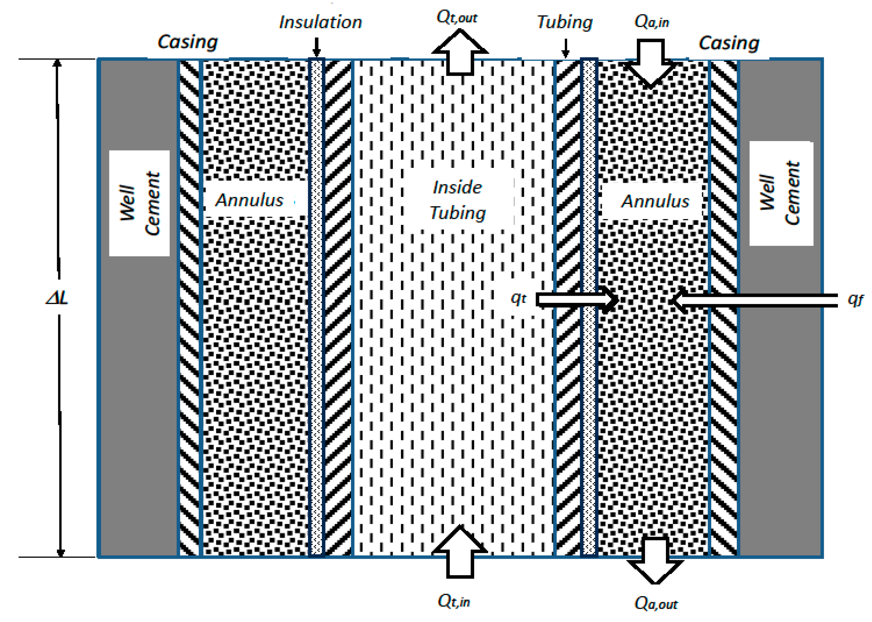
Q_a,in = heat transfer through the annular element due to the annulus fluid, J.
q_f = heat transfer from the formation to the annulus, J.
q_t = heat transfer from the tubing to the annulus, J.
Q_a,out = heat getting out of the annular element by the annulus fluid, J.
Q_a,change = change of heat in the annulus fluid in the element, J.

For the returning fluid inside the tubing, the heat balance is expressed:

Q_{t, i n} - q_{t} - Q_{t, o u t} = Q_{t, c h a n g e}

(2)

where

Q_t,in = heat coming into the tubing element by the tubing fluid, J.
q_t = heat transfer from the annulus to the tubing, J.
Q_t,out = heat coming out of the tubing element by the tubing fluid, J.
Q_t,change = change of heat in the tubing fluid in the element, J.

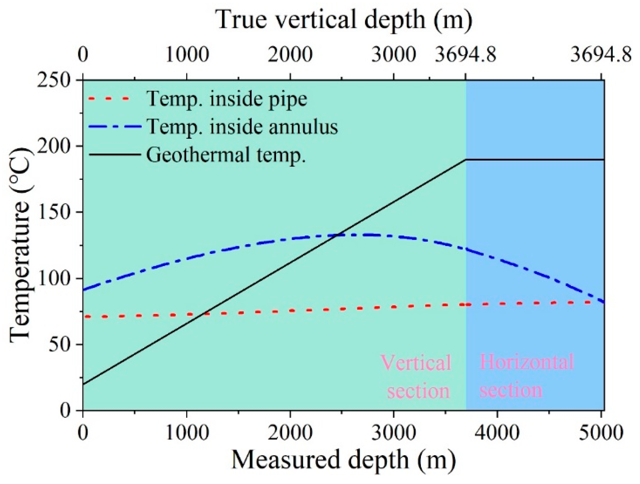
After going through a tedious procedure of mathematical formulation, analytical solutions for fluid temperature profiles in the tubing and the annular space were obtained. Detailed derivations are shown in Appendix A.

For the wellbore configuration shown in Figure 2, Equations (A37) and (A38) in Appendix A have to be applied to the vertical section and the horizontal section sequentially. The temperature difference between the water inside tubing and that in the annulus at the bottom of the horizontal wellbore is zero, while the temperature difference between the water inside tubing and that in the annulus at the end of the vertical section has to be computed using a numerical procedure (trial-and-error) to meet the requirements of both sections.

3. Field Case Study

The analytical model was applied to an end-of-life horizontal oil well in the Northwest region of Louisiana in the United States. Basic well data are summarized in Table 1.

Data was collected from Drillinginfo for two shale formations: the Haynesville shale and the Eagle-Ford shale. The Haynesville shale spans both Texas and Louisiana, but for this study, the North-west Louisiana section was specifically focused on. The dataset comprises information from approximately 1673 wells drilled and completed, with a detailed examination conducted on 709 of these wells. The earliest wells in the dataset date back to around 2006. Of these, about 189 wells are labeled as inactive, primarily shorter wells drilled in the early stages of play development. Although these shorter wells are not suitable for large-scale geothermal development, a pair of them could serve well for a pilot test. The vertical and horizontal sections of the well chosen for this study have the same casing and tubing size. Polyurethane foam is assumed to use for tubing insulation. It has a thermal conductivity between 0.02 and 0.04 W/(m·°C), averaged at 0.03 W/(m·°C). A case study was conducted using the data in Table 1 for both reverse circulation and direct circulation of water at an injection of 397.5 m³/day.

Figure 4 presents computed temperature profiles for reverse circulation, the temperature of water returned to the surface is about 124 °C. It indicates that the injected water in the annulus is cooled down near the surface and heated up in the deeper depth by the surrounding formation rock. The temperature of the water inside the tubing drops as it flows toward the surface due to the loss of heat into the water in the annulus.

Figure 5 shows computed temperature profiles using the direct circulation model, the temperature of water returned to the surface is about 92 °C, which is much lower than that in the reverse circulation. It indicates that the injected water in the tubing is heated up very slowly by the water in the annulus. The temperature of water in the annulus drops as it flows toward the surface due to the heat loss into the formation rock and the water in the tubing.

The impact of hot water temperature on the efficiency of geothermal power generation lies mainly in the fact that higher temperatures result in the production of steam with higher pressure and energy. This enhances the overall efficiency of the entire power generation process, including the efficiency of turbine propulsion and the conversion of mechanical energy to electricity by the generator. Therefore, higher temperature hot water generally signifies higher efficiency in geothermal power generation.

Building upon the significance of hot water temperature, the range of temperatures plays a crucial role in determining geothermal power generation efficiency. In low-temperature geothermal power plants, where the water is typically below 150 °C, the efficiency tends to be relatively low, typically ranging from 10% to 15%. Medium-temperature geothermal power plants, with hot water ranging from approximately 150 °C to 200 °C, exhibit efficiencies generally falling within the range of 10% to 20%. For high-temperature geothermal power plants, characterized by hot water temperatures above 200 °C, the efficiency can reach levels exceeding 20%, contingent on the specific geothermal resources and technologies employed [15,16,17,18].

In this case study, the hot water temperatures obtained from both circulation patterns are below 150 °C, making them suitable for low-temperature geothermal power plants. Since (124 °C − 92 °C)/92 °C = 0.35, it is concluded that reverse circulation is 35% more efficient than direct circulation. This is because water loses heat energy into the surrounding rock on its way returning to the surface through wellbore annulus. Therefore, only the reverse circulation method is employed in the sensitivity analysis that follows. It’s worth noting that while both temperatures mentioned apply specifically to low-temperature geothermal power plants, a higher water temperature generally corresponds to higher electricity generation efficiency. Therefore, this calculation result is conservative.

4. Sensitivity Analysis

A sensitivity analysis was performed using the data set in Table 1 to identify key factors affecting the heat energy productivity of converted wells. The value of each parameter employed for the results presented in each figure is as listed in Table 1, unless otherwise specified in the individual figure legends. Sensitized parameters include water injection rate, horizontal wellbore length, reservoir temperature, temperature of injected water, and thermal conductivity and thickness of tubing insulation.

Figure 6 shows the effects of water injection rate and horizontal wellbore length (L) on the heat energy productivity of the well. It indicates that the water injection rate is a dominating factor affecting well productivity. The trend does not level off even water injection rate is greater than 2384.8 m³/day which is almost the upper limit of the water flow rate for the 2.441″ ID tubing. A high flow rate causes high pressure at the bottom hole due to excessive flow friction, which may cause a leak of the casing, resulting in loss of injected water to the formation rock and thus lower temperature around the wellbore. The effect of horizontal wellbore length seems to have negligible impact on the well productivity in the low-injection rate region. This is because short horizontal wellbores can provide adequate heat to the water at low flow rates.

Figure 7 illustrates the effects of water temperature and reservoir temperature (T_res) on the heat energy productivity of the well. It indicates that well productivity is nearly proportional to these two temperatures, but less sensitive to the temperature of the injected water. This is because the injected water is heated up by the surrounding rock anyway no matter if its temperature is low or high at the surface.

Figure 8 presents the effects of thermal conductivity (K_n) and thickness of the tubing insulation layer on the heat energy productivity of the well. It implies that well productivity is more sensitive to the thermal conductivity in a thin layer than in a thick layer of insulation. This is expected because thick layers of insulation efficiently block heat transfer even if the thermal conductivity is high.

5. Discussion

The temperatures in the annulus and tubing are influenced by various factors including the geothermal gradient, wellbore and tubing string geometries, thermal conductivities of the cement sheath and tubing insulation, density and heat capacity of water, surface temperature of injected water, and water injection rate. The data presented in the preceding section underscores the promising scenarios associated with converting oil/gas wells into geothermal wells for heat energy production, particularly with the implementation of the reverse circulation pattern.

This model can conveniently assist engineers in evaluating how much more efficient the reverse circulation is compared to the direct circulation in specific scenarios. Taking into account economic factors comprehensively, it aids in determining which approach is more favorable, facilitating the decision-making process.

Even though the reverse circulation method is more efficient than the direct circulation method, there are situations where it may not be the optimal solution, considering the need to mitigate circulation pressure in the annulus and reduce the risk of water leakage into the geothermal pay zone. In such cases, the direct circulation method should be employed. Before implementing the reverse circulation, engineers should determine pressure safety thresholds and assess the optimal operational parameters.

The economic viability of the well is directly tied to the scale of the project. A low number of wells may not justify conversion due to installation and maintenance costs. Further assessment work is required for both technical and economic analyses after the energy productivity assessment demonstrates promise.

Expanding on the economic considerations, the conversion of abandoned oil wells into geothermal wells involves significant retrofitting process costs. This includes expenses related to modifying existing infrastructure, installing geothermal equipment, and ensuring compliance with environmental regulations. Economic viability is contingent on multiple factors, such as the potential geothermal resource’s temperature and capacity, available government incentives or subsidies, and the long-term revenue generated from geothermal power production. A critical step in determining economic feasibility involves evaluating the return on investment and the payback period for converting abandoned oil wells into geothermal wells.

6. Limitations

In this work, the working fluid is water, and it is assumed that the specific heat capacity of water is constant. However, it’s important to note that the specific heat capacity of water does vary with temperature. As a general guideline, the specific heat capacity tends to decrease slightly as the temperature increases. For accurate calculations, especially in scientific and engineering contexts where precise temperature-dependent properties are essential, specific heat capacity data tables may be consulted to account for these variations over different temperature ranges. The vertical well section can be artificially divided into segments, and calculations can be performed using different specific heat capacities. If using a different working fluid, the specific heat capacity may be more temperature-sensitive. When utilizing this model, careful analysis of the impact of specific heat capacity variations with temperature is advisable.

In addition, one of assumptions made in this work is that the temperature of the formation rock is not influenced by the injected water. However, in reality, this represents a limitation of the established model. As the working fluid is continuously injected, the formation temperature will decrease, leading to a reduction in the heating efficiency of the working fluid. Meanwhile, over the long term, the lost heat is replenished by adjacent areas through heat conduction. Introducing the temporal variations of formation temperature and working fluid temperature with time into the model can enhance its accuracy in the future study.

7. Applications

The findings of this study can have broader implications beyond the oil and gas industry. The promising result implies that the geothermal energy sector can expand from the transitional volcanic settings such as Hawaii, Rocky Mountain, and Yellowstone in the United States, where oil and gas are seldom found, to sedimentary basins such as the Gulf Coast region where thousands of oil and gas wells are at their end-of-life condition. Real-world implementation of the results from this and future research work in this area can promote profitable transitin from the polusive fossil energy to the cleaner geothermal energy. This will greatly impact the life of mankind economically and environmentally.

It is crucial to acknowledge that energy productivity represents just one facet of feasibility assessment. In addition to technical feasibility, the viability of the well in challenging economic conditions requires careful consideration. Technical feasibility encompasses a range of factors, including the cost of sealing well perforations, the expense of using tubing strings with insulation layers, the geological integrity of the well structure, and the adaptability of existing oil well infrastructure for geothermal conversion.

Because geothermal energy is everywhere in the earth, there is no limitation in principle, that hinders implementation of the model. However, geographical locations with high-geothermal gradients are preferable to apply the new model due to the reduced cost of drilling for reaching hot geothermal zones. In geographical locations with low-geothermal gradients, application of the new model will require additional investment to drilling deeper for reaching hot geothermal zones.

8. Conclusions

An analytical model was developed in this study for predicting the energy productivity of geothermal wells converted from end-of-life oil and gas wells with reverse circulation. A case study was conducted using the data for a well in North-west Louisiana to compare direct circulation and reverse circulation scenarios. A sensitivity study was performed with the developed model to identify major factors affecting well productivity. The following conclusions are drawn.

(1): Reverse circulation is more efficient than direct circulation for improving the heat-energy productivity of geothermal wells converted from oil/gas wells. In the studied well case, the improvement is up to 35%. If water injection pressure is not a concern, the reverse circulation method should be employed in field operations.
(2): The result of sensitivity analysis indicates that well productivity is proportional to the water injection rate with a trend that does not level off even water injection rate is over 2000 m³/day. This model-predicted trend may be optimistic because the model does not consider the effect of water flow rate on the change of rock temperature around the wellbore.
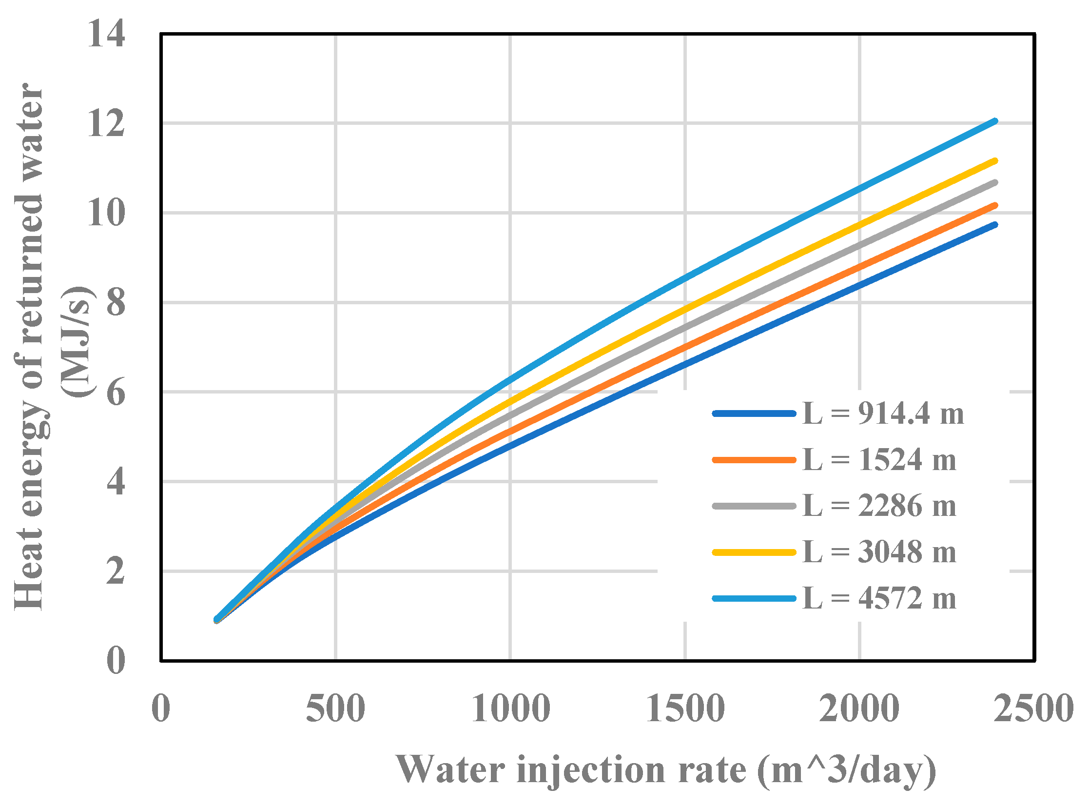
(3): The result of sensitivity analysis indicates that well productivity increases with the length of the horizontal wellbore that promotes heat transfer from the pay zone to the water stream. But the effect of horizontal wellbore length is less in the low-injection rate region than in the high-injection rate region. This is because short horizontal wellbores can provide adequate energy to heat water streams at low flow rates.
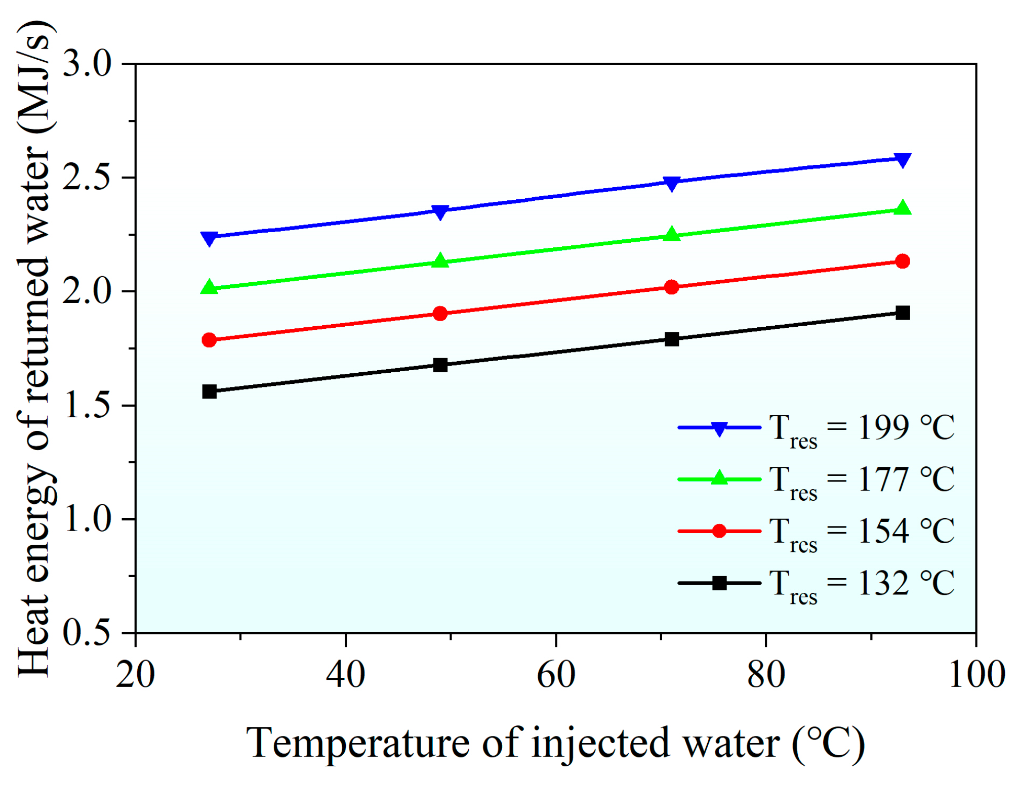
(4): The result of sensitivity analysis indicates that both the injected water temperature and the reservoir temperature affect the heat-energy productivity of the well. Well productivity is nearly proportional to the reservoir temperature which provides more heat energy. Well productivity is less sensitive to the temperature of the surface-injected water. This is because the injected water is heated up by the surrounding rock no matter if its temperature is low or high.
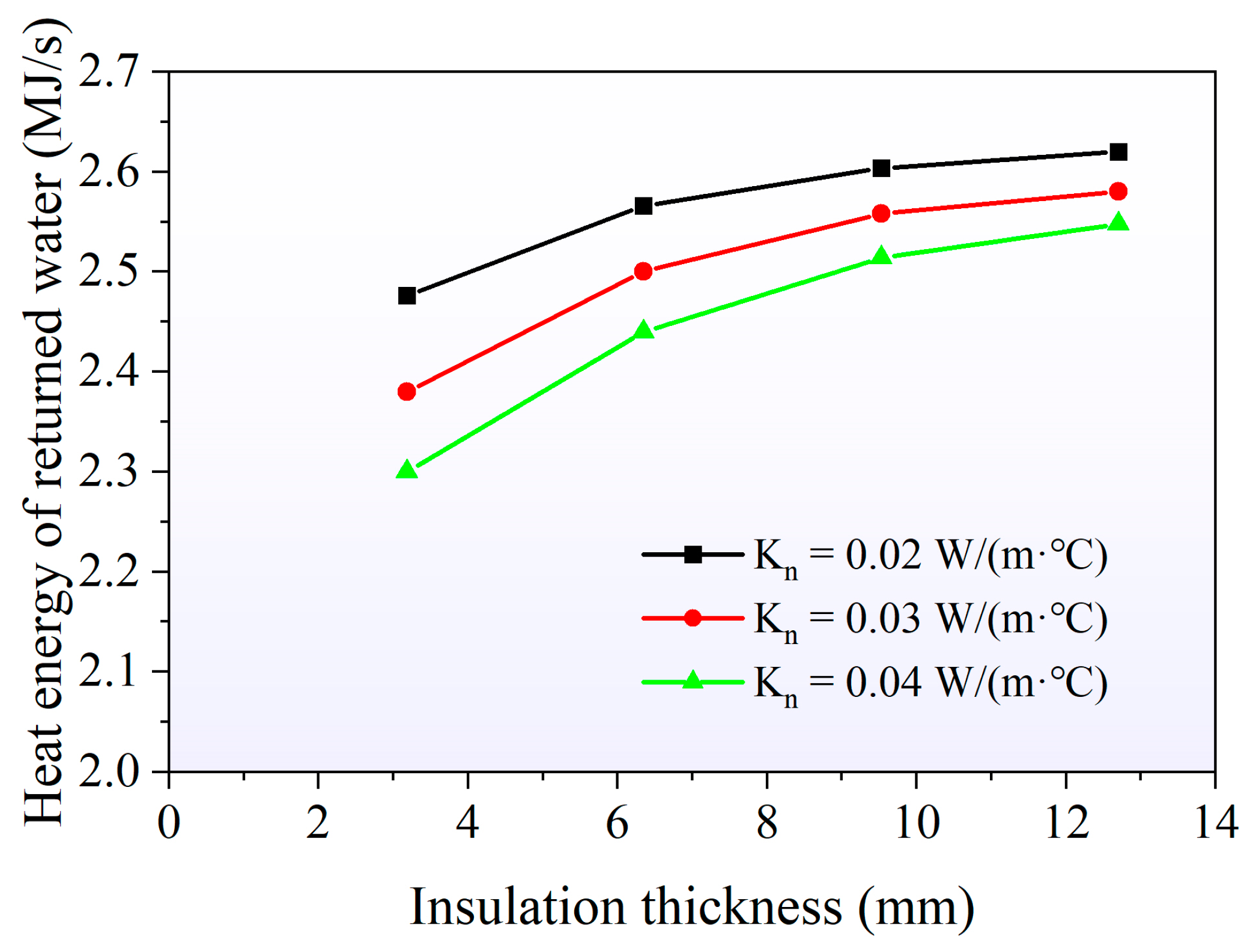
(5): The result of sensitivity analysis indicates well productivity increases with reduced thermal conductivity of tubing insulation and increased thickness of the insulation layer. The effect of thermal conductivity is more pronounced for thin insulation layers than for thick insulation layers because thick layers of insulation efficiently block heat transfer even if the thermal conductivity is high.
(6): Future research toward development of ready-to-use technology should consider the temporal variation of geothermal reservoir temperatures over extended periods. Additionally, there is a need for comparative analyses of the performance of different working fluids, considering the optimization of heating efficiency and economic benefits when multiple sensitized parameters interact. Exploring these aspects will contribute to a deeper understanding of the dynamics of geothermal reservoirs and will facilitate the identification of optimal conditions for both heating efficiency and economic viability under the influence of various sensitive factors.
(7): The findings of this study can have broader implications beyond the oil and gas industry. This study suggests that the geothermal energy sector be expanded from the transitional volcanic settings where oil and gas are seldom found to sedimentary basins of rich oil and gas resources. This should promote the smooth transition from the pollusive fossil energy to the cleaner geothermal energy.

Author Contributions

Conceptualization, B.G.; Formal analysis, P.Z. All authors have read and agreed to the published version of the manuscript.

Funding

This research received no external funding.

Data Availability Statement

No new data were created or analyzed in this study. Data sharing is not applicable to this article.

Acknowledgments

The authors are grateful to the Energy Institute of Louisiana at the University of Louisiana at Lafayette for its financial support to this research work.

Conflicts of Interest

The authors declare no conflicts of interest.

Nomenclature

C_a	heat capacity of the annulus fluid, J/(kg·°C)
C_t	heat capacity of the tubing fluid, J/(kg·°C)
D_c	outer diameter of casing, m
D_t	outer diameter of tubing insulation, m
D_w	outer diameter of cement, m
d_tn	inner diameter of tubing insulation, m
G_g	geothermal gradient, °C/m
K_c	heat conductivity of cement sheath, W/(m·°C)
K_t	heat conductivity of tubing insulation, W/(m·°C)
L	measured depth, m
${\dot{m}}_{a}$	mass flow rate of the annulus fluid, kg/s
${\dot{m}}_{t}$	mass flow rate of the tubing fluid, kg/s
T_g0	geothermal temperature at surface soil, °C
T_a	fluid temperature inside annulus, °C
T_t	fluid temperature inside tubing, °C
ΔT	difference between the temperatures inside tubing and annulus, °C

Appendix A. Derivation of the Heat Transfer Model for Wells with Reverse Circulation

Appendix A.1. Assumptions

The following assumptions are made in deriving the heat transfer model:

The geothermal gradient does not change during borehole fluids circulation.
The thermal conductivities of the casing and the tubing strings are infinite.
The fluid heat capacity remains constant.
The heat buildup from friction in this process is trivial.

Appendix A.2. Governing Equations

Through mathematical derivation consistent with conservation laws, a system of two coupled differential equations has been established to characterize the temperature distributions in the annular space and inner pipe.

Consider the wellbore element shown in Figure 3. For the fluid in the annulus, heat energy balance is expressed as:

Q_{a, i n} + q_{f} + q_{t} - Q_{a, o u t} = Q_{a, c h a n g e}

(A1)

where

Q_a,in = Heat transfer through the annular element due to the annulus fluid, J.
q_f = Heat transfer from the formation to the annulus, J.
q_t = Heat transfer from the tubing to the annulus, J.
Q_a,out = Heat getting out of the annular element by the annulus fluid, J.
Q_a,change = Heat change in the annulus fluid in the element, J.

The heat getting into the annular element is described as:

Q_{a, i n} = C_{a} {\dot{m}}_{a} T_{a, L} Δ t

(A2)

where

C_a = Heat capacity of the annulus fluid, J/(kg·°C).
${\dot{m}}_{a}$ = Mass flow rate of the annulus fluid, kg/s.
T_a,L = Temperature of the annulus fluid at depth L, °C.
$Δ t$ = Time change, s.

The heat transferring from the formation to the annulus is formulated as:

q_{f} = π D_{c} Δ L K_{c} (\frac{\partial T_{c}}{\partial r}) Δ t

(A3)

where

D_c = Outer diameter of casing, m.
K_c = Heat conductivity of cement sheath, W/(m·°C).

The heat transferring from the tubing to the annulus takes the form:

q_{t} = π D_{t} Δ L K_{t} (- \frac{\partial T_{t b}}{\partial r}) Δ t

(A4)

where

D_t = Outer diameter of the tubing insulation, m.
K_t = Heat conductivity of the tubing insulation, W/(m·°C).

The heat coming out of the element is expressed as:

Q_{a, o u t} = C_{a} {\dot{m}}_{a} T_{a, L + Δ L} Δ t

(A5)

The heat change in the annulus is characterized by:

Q_{a, c h a n g e} = C_{a} ρ_{a} A_{a} Δ L Δ T_{a}

(A6)

where

A_a = Area of the annular space, m².
$ρ_{a}$ = Density of the annular fluid, kg/m³.

Submitting Equations (A2)–(A6) into (A1) gives:

C_{a} {\dot{m}}_{a} T_{a, L} Δ t + π D_{c} Δ L K_{c} (\frac{\partial T_{c}}{\partial r}) Δ t + π D_{t} Δ L K_{t} (- \frac{\partial T_{t b}}{\partial r}) Δ t - C_{a} {\dot{m}}_{a} T_{a, L + Δ L} Δ t = C_{a} ρ_{a} A_{a} Δ L Δ T_{a}

(A7)

To simplify (A7) yields:

C_{a} {\dot{m}}_{a} Δ t (T_{a, L} - T_{a, L + Δ L}) + π D_{c} Δ L K_{c} (\frac{\partial T_{c}}{\partial r}) Δ t + π D_{t} Δ L K_{t} (- \frac{\partial T_{t b}}{\partial r}) Δ t = C_{a} ρ_{a} A_{a} Δ L Δ T_{a}

(A8)

In the cement, we have:

\frac{\partial T_{c}}{\partial r} = \frac{T_{g} - T_{a}}{\frac{D_{w} - D_{c}}{2}}

(A9)

where

T_g = Formation temperature, °C.
D_w = Outer diameter of cement, m.
D_c = Outer diameter of casing, m.

For the tubing insulation, we obtain:

\frac{\partial T_{t b}}{\partial r} = \frac{T_{a} - T_{t}}{\frac{D_{t} - d_{t n}}{2}}

(A10)

where

T_t = Temperature of tubing, °C.
D_t = Outer diameter of tubing insulation, m.
d_tn = Inner diameter of tubing insulation, m.

By substituting Equations (A9) and (A10) into Equation (A8), and dividing across all terms by ‘

Δ L \cdot Δ t

’, we obtain:

C_{a} {\dot{m}}_{a} \frac{(T_{a, L} - T_{a, L + Δ L})}{Δ L} + 2 π D_{c} K_{c} \frac{T_{g} - T_{a}}{D_{w} - D_{c}} - 2 π D_{t} K_{t} \frac{T_{a} - T_{t}}{D_{t} - d_{t}_{n}} = \frac{C_{a} ρ_{a} A_{a} Δ T_{a}}{Δ t}

(A11)

- C_{a} {\dot{m}}_{a} \frac{\partial T_{a}}{\partial L} + 2 π D_{c} K_{c} \frac{T_{g} - T_{a}}{D_{w} - D_{c}} - 2 π D_{t} K_{t} \frac{T_{a} - T_{t}}{D_{t} - d_{t}_{n}} = C_{a} ρ_{a} A_{a} \frac{\partial T_{a}}{\partial t}

(A12)

where

A_{a} = \frac{π}{4} (d_{c}^{2} - D_{t}^{2})

(A13)

Equation (A12) can be simplified to:

\frac{\partial T_{a}}{\partial L} + α \frac{\partial T_{a}}{\partial t} + β (T_{g} - T_{a}) + γ (T_{a} - T_{t}) = 0

(A14)

where

α = \frac{π ρ_{a} (d_{c}^{2} - D_{t}^{2})}{4 {\dot{m}}_{a}}

(A15)

β = - \frac{2 π D_{c} K_{c}}{C_{a} {\dot{m}}_{a} (D_{w} - D_{c})}

(A16)

γ = \frac{2 π D_{t} K_{t}}{C_{a} {\dot{m}}_{a} (D_{t} - d_{t n})}

(A17)

For geothermal temperature,

T_{g} = T_{g 0} + G_{g} L

(A18)

where

T_g0 = Geothermal temperature at surface soil, °C.
G_g = Geothermal gradient, °C/m.
L = Depth, m.

For an infinitesimal element length, the governing equation for the fluid in the annulus takes the form:

\frac{\partial T_{a}}{\partial L} + α \frac{\partial T_{a}}{\partial t} + (γ - β) T_{a} - γ T_{t} + β G_{g} L + β T_{g 0} = 0

(A19)

For fluid inside the tubing, the heat balance is expressed:

Q_{t, i n} - q_{t} - Q_{t, o u t} = Q_{t, c h a n g e}

(A20)

where

Q_t,in = Heat coming into the tubing element by the tubing fluid, J.
q_t = Heat transfer from the annulus to the tubing, J.
Q_t,out = Heat coming out of the tubing element by the tubing fluid, J.
Q_t,change = Change of heat in the tubing fluid in the element, J.

The heat coming into the fluid inside the tubing element is described as follows:

Q_{t, i n} = C_{t} {\dot{m}}_{t} T_{t, L + Δ L} Δ t

(A21)

where

C_t = Heat capacity of the tubing fluid, J/(kg·°C).
${\dot{m}}_{t}$ = Mass flow rate of the tubing fluid, kg/s.
T_t,L = Temperature of the tubing fluid at depth L, °C.
$Δ t$ = Time change, s.

The heat getting out of the fluid inside the tubing element is formulated as:

Q_{t, o u t} = C_{t} {\dot{m}}_{t} T_{t, L} Δ t

(A22)

The heat change in the tubing element obeys:

Q_{t, c h a n g e} = C_{t} ρ_{t} A_{t} Δ L Δ T_{t}

(A23)

where

A_t = Area of tubing, m².
$ρ_{a}$ = Density of the tubing fluid, kg/m³.

Substituting Equations (A21)–(A23) into (A20) yields:

C_{t} {\dot{m}}_{t} T_{t, L + Δ L} Δ t - π D_{t} Δ L K_{t} (- \frac{\partial T_{t b}}{\partial r}) Δ t - C_{t} {\dot{m}}_{t} T_{t, L} Δ t = C_{t} ρ_{t} A_{t} Δ L Δ T_{t}

(A24)

Simplifying (A24) yields:

C_{t} {\dot{m}}_{t} Δ t (T_{t, L + Δ L} - T_{t, L}) - π D_{t} Δ L K_{t} (- \frac{\partial T_{t b}}{\partial r}) Δ t = C_{t} ρ_{t} A_{t} Δ L Δ T_{t}

(A25)

Submitting (A10) into (A25) yields:

C_{t} {\dot{m}}_{t} Δ t (T_{t, L + Δ L} - T_{t, L}) - π D_{t} Δ L K_{t} (\frac{T_{a} - T_{t}}{\frac{D_{t} - d_{t n}}{2}}) Δ t = C_{t} ρ_{t} A_{t} Δ L Δ T_{t}

(A26)

Dividing all terms by ‘

Δ L \cdot Δ t

’ gives:

\frac{C_{t} {\dot{m}}_{t} (T_{t, L + Δ L} - T_{t, L})}{Δ L} + 2 π D_{t} K_{t} (\frac{T_{a} - T_{t}}{D_{t} - d_{t n}}) = \frac{C_{t} ρ_{t} A_{t} Δ T_{t}}{Δ t}

(A27)

Equation (A27) can be simplified as:

C_{t} {\dot{m}}_{t} \frac{\partial T_{t}}{Δ L} + 2 π D_{t} K_{t} (\frac{T_{a} - T_{t}}{D_{t} - d_{t n}}) = C_{t} ρ_{t} A_{t} \frac{\partial T_{t}}{\partial t}

(A28)

For an infinitesimal element length, the governing equation for the fluid inside the tubing is formulated as:

\frac{\partial T_{t}}{\partial L} - a \frac{\partial T_{t}}{\partial t} + b T_{a} - b T_{t} = 0

(A29)

where

a = - \frac{π ρ_{t} d_{t}^{2}}{4 {\dot{m}}_{t}}

(A30)

b = \frac{2 π D_{t} K_{t}}{C_{t} {\dot{m}}_{t} (D_{t} - d_{t n})}

(A31)

Appendix A.3. Boundary Conditions

The model is subject to two boundary conditions. For the annular flow, the fluid temperature inside the annulus at surface is the same as that of the injected fluid, which means:

T_{a} = T_{a 0} @ L = 0

(A32)

For the tubing flow, the temperature of the fluid inside the tubing is the same as that of the fluid in the annulus at the bottom. To make the model general for handling systems with segments of different geometries, inclination angles, and insulation properties, a temperature change ΔT is considered. The boundary condition at the lower end of a segment is expressed as:

T_t =T_a + ΔT @ L = L_max

(A33)

where L_max is the maximum length of the segment.

Appendix A.4. Solution

For the steady state condition:

\frac{\partial T_{a}}{\partial t} = 0, \frac{\partial T_{t}}{\partial t} = 0

(A34)

Therefore, the governing Equations (A19) and (A29) can be simplified as:

\frac{\partial T_{a}}{\partial L} + (γ - β) T_{a} - γ T_{t} + β G_{g} L + β T_{g 0} = 0

(A35)

\frac{\partial T_{t}}{\partial L} + b T_{a} - b T_{t} = 0

(A36)

The solutions of PDEs (A35) and (A36) take the form:

T_{a} = F C_{1} e^{r_{1} L} + G C_{2} e^{r_{2} L} + E L + J

(A37)

T_{t} = \frac{C_{1}}{q^{2}} e^{r_{1} L} + \frac{C_{2}}{q^{2}} e^{r_{2} L} + E L + D

(A38)

where all terms used in Equations (A37) and (A38) and the equations for calculating these terms are defined as follows:

a^{'} = γ - β

(A39)

c = β G_{g}

(A40)

d = β T_{g 0}

(A41)

p = a^{'} - b

(A42)

q = β b

(A43)

r_{1} = \frac{- p + \sqrt{p^{2} - 4 q}}{2}

(A44)

r_{2} = \frac{- p - \sqrt{p^{2} - 4 q}}{2}

(A45)

Q = p b c

(A46)

D = \frac{d b q - Q}{q^{2}}

(A47)

E = \frac{c}{β}

(A48)

F = \frac{b - r_{1}}{b q^{2}}

(A49)

G = \frac{b - r_{2}}{b q^{2}}

(A50)

J = D - \frac{c}{q}

(A51)

K = e^{r_{1} L_{\max}} (F - \frac{1}{q^{2}})

(A52)

R = e^{r_{2} L_{\max}} (G - \frac{1}{q^{2}})

(A53)

S = D - J - Δ T

(A54)

C_{1} = \frac{R (A - J) - S G}{F R - G K}

(A55)

C_{2} = \frac{K (A - J) - S F}{G K - F R}

(A56)

References

Capobianco, N.; Basile, V.; Loia, F.; Vona, R. End-of-Life Management of Oil and Gas Offshore Platforms: Challenges and Opportunities for Sustainable Decommissioning. Sinergie Ital. J. Manag. 2022, 40, 299–326. [Google Scholar] [CrossRef]
Dachis, B.; Shaffer, B.; Thivierge, V. All’s Well That Ends Well: Addressing End-of-Life Liabilities for Oil and Gas Wells; C.D. Howe Institute: Toronto, ON, Canada, 2017; p. 492. [Google Scholar]
Santos, L.; Taleghani, A.D.; Elsworth, D. Repurposing Abandoned Wells for Geothermal Energy: Current Status and Future Prospects. Renew. Energy 2022, 194, 1288–1302. [Google Scholar] [CrossRef]
Kaiser, M.J.; Dodson, R. Cost of Plug and Abandonment Operations in the Gulf of Mexico. Mar. Technol. Soc. J. 2007, 41, 12–22. [Google Scholar] [CrossRef]
Vrålstad, T.; Saasen, A.; Fjær, E.; Øia, T.; Ytrehus, J.D.; Khalifeh, M. Plug & Abandonment of Offshore Wells: Ensuring Long-Term Well Integrity and Cost-Efficiency. J. Pet. Sci. Eng. 2019, 173, 478–491. [Google Scholar]
Caulk, R.A.; Tomac, I. Reuse of Abandoned Oil and Gas Wells for Geothermal Energy Production. Renew. Energy 2017, 112, 388–397. [Google Scholar] [CrossRef]
Nian, Y.-L.; Cheng, W.-L. Insights into Geothermal Utilization of Abandoned Oil and Gas Wells. Renew. Sustain. Energy Rev. 2018, 87, 44–60. [Google Scholar] [CrossRef]
Wight, N.M.; Bennett, N.S. Geothermal Energy from Abandoned Oil and Gas Wells Using Water in Combination with a Closed Wellbore. Appl. Therm. Eng. 2015, 89, 908–915. [Google Scholar] [CrossRef]
Hossain, M.F. In Situ Geothermal Energy Technology: An Approach for Building Cleaner and Greener Environment. J. Ecol. Eng. 2016, 17, 49–55. [Google Scholar] [CrossRef]
Kuo, G. Geothermal Energy. World Futur. Rev. 2012, 4, 5–7. [Google Scholar] [CrossRef]
Rybar, P. Geothermal Energy Sources and Possibilities of Their Exploitation. Acta Montan. Slovaca 2007, 12, 31–41. [Google Scholar]
Blackwell, D.D.; Wisian, K.W.; Richards, M.C.; Steele, J.L. Geothermal Resource/Reservoir Investigations Based on Heat Flow and Thermal Gradient Data for the United States; USDOE Idaho Operations Office: Idaho Falls, ID, USA; Southern Methodist: Dallas, TX, USA, 2000.
Majumdar, U.; Cook, A.E.; Scharenberg, M.; Burchwell, A.; Ismail, S.; Frye, M.; Shedd, W. Semi-Quantitative Gas Hydrate Assessment from Petroleum Industry Well Logs in the Northern Gulf of Mexico. Mar. Pet. Geol. 2017, 85, 233–241. [Google Scholar] [CrossRef]
Nicot, J.-P. A Survey of Oil and Gas Wells in the Texas Gulf Coast, USA, and Implications for Geological Sequestration of CO₂. Environ. Geol. 2009, 57, 1625–1638. [Google Scholar] [CrossRef]
Gosnold, W.; Mann, M.; Salehfar, H. The UND-CLR Binary Geothermal Power Plant. GRC Trans. 2017, 41, 1824–1834. [Google Scholar]
Gosnold, W.; Abudureyimu, S.; Tisiryapkina, I.; Wang, D.; Ballesteros, M. The Potential for Binary Geothermal Power in the Williston Basin. GRC Trans. 2019, 43, 114–126. [Google Scholar]
Gosnold, W.; Ballesteros, M.; Wang, D.; Crowell, J. Using Geothermal Energy to Reduce Oil Production Costs. GRC Trans. 2020, 44. [Google Scholar]
Abudureyimu, S. Geothermal Energy from Repurposed Oil and Gas Wells in Western North Dakota. Master’s Thesis, University of North Dakota, Grand Forks, ND, USA, 2020; pp. 51–74. [Google Scholar]
Haghighi, A.; Pakatchian, M.R.; Assad, M.E.H.; Duy, V.N.; Alhuyi Nazari, M. A Review on Geothermal Organic Rankine Cycles: Modeling and Optimization. J. Therm. Anal. Calorim. 2021, 144, 1799–1814. [Google Scholar] [CrossRef]
Nami, H.; Nemati, A.; Fard, F.J. Conventional and Advanced Exergy Analyses of a Geothermal Driven Dual Fluid Organic Rankine Cycle (ORC). Appl. Therm. Eng. 2017, 122, 59–70. [Google Scholar] [CrossRef]
Bu, X.; Ma, W.; Li, H. Geothermal Energy Production Utilizing Abandoned Oil and Gas Wells. Renew. Energy 2012, 41, 80–85. [Google Scholar] [CrossRef]
Jello, J.; Baser, T. Utilization of Existing Hydrocarbon Wells for Geothermal System Development: A Review. Appl. Energy 2023, 348, 121456. [Google Scholar] [CrossRef]
Li, J.; Guo, B.; Li, B. A Closed Form Mathematical Model for Predicting Gas Temperature in Gas-Drilling Unconventional Tight Reservoirs. J. Nat. Gas Sci. Eng. 2015, 27, 284–289. [Google Scholar] [CrossRef]
Liu, Y.; Shan, L. Numerical solutions of heat transfer problems in gas production from seabed gas hydrates. J. Pet. Sci. Eng. 2020, 188, 106824. [Google Scholar] [CrossRef]
Fu, C.; Guo, B.; Shan, L.; Lee, J. Mathematical Modeling of Heat Transfer in Y-Shaped Well Couples for Developing Gas Hydrate Reservoirs Using Geothermal Energy. J. Nat. Gas Sci. Eng. 2021, 96, 104325. [Google Scholar] [CrossRef]

Figure 1. Distribution and grade of geothermal energy resources in the conterminous United States [12].

Figure 2. A sketch of a geothermal well converted from a horizontal oil/gas well.

Figure 3. Sketch of heat transfer in a wellbore element.

Figure 4. Computed temperature profiles for reverse circulation.

Figure 5. Computed temperature profiles for direct circulation.

Figure 6. Effects of water injection rate and horizontal wellbore length on heat energy productivity of well.

Figure 7. Effects of injected water temperature and reservoir temperature on heat energy productivity of well.

Figure 8. Effects of tubing insulation properties on heat energy productivity of the well.

Table 1. A summary of base data used in the project.

Parameters	Value	Unit
Surface soil temperature	20	°C
Geothermal temperature in the pay zone	190.6	°C
Well total depth	5030.6	m
Horizontal wellbore length	1338.7	m
Wellbore diameter	0.203	m
Casing OD	0.140	m
Casing ID	0.128	m
Tubing OD	0.073	m
Tubing ID	0.062	m
Tubing insulation thickness	0.003	m
Thermal conductivity of cement sheath	0.5	W/(m·°C)
Thermal conductivity of tubing insulation	0.03	W/(m·°C)
Temperature of injected fluid at surface	71.1	°C
Inclination angle of horizontal wellbore	90	degrees
Heat capacity of injected water	4184	J/(kg·°C)
Density of injected water	1000	kg/m³
Water injection rate	397.5	m³/day

Disclaimer/Publisher’s Note: The statements, opinions and data contained in all publications are solely those of the individual author(s) and contributor(s) and not of MDPI and/or the editor(s). MDPI and/or the editor(s) disclaim responsibility for any injury to people or property resulting from any ideas, methods, instructions or products referred to in the content.

© 2024 by the authors. Licensee MDPI, Basel, Switzerland. This article is an open access article distributed under the terms and conditions of the Creative Commons Attribution (CC BY) license (https://creativecommons.org/licenses/by/4.0/).

Share and Cite

MDPI and ACS Style

Zhang, P.; Guo, B. A Feasibility Assessment of Heat Energy Productivity of Geothermal Wells Converted from Oil/Gas Wells. Sustainability 2024, 16, 768. https://doi.org/10.3390/su16020768

AMA Style

Zhang P, Guo B. A Feasibility Assessment of Heat Energy Productivity of Geothermal Wells Converted from Oil/Gas Wells. Sustainability. 2024; 16(2):768. https://doi.org/10.3390/su16020768

Chicago/Turabian Style

Zhang, Peng, and Boyun Guo. 2024. "A Feasibility Assessment of Heat Energy Productivity of Geothermal Wells Converted from Oil/Gas Wells" Sustainability 16, no. 2: 768. https://doi.org/10.3390/su16020768

Note that from the first issue of 2016, this journal uses article numbers instead of page numbers. See further details here.

Article Menu

A Feasibility Assessment of Heat Energy Productivity of Geothermal Wells Converted from Oil/Gas Wells

Abstract

1. Introduction

2. Mathematical Model

3. Field Case Study

4. Sensitivity Analysis

5. Discussion

6. Limitations

7. Applications

8. Conclusions

Author Contributions

Funding

Data Availability Statement

Acknowledgments

Conflicts of Interest

Nomenclature

Appendix A. Derivation of the Heat Transfer Model for Wells with Reverse Circulation

Appendix A.1. Assumptions

Appendix A.2. Governing Equations

Appendix A.3. Boundary Conditions

Appendix A.4. Solution

References

Share and Cite

Article Metrics

Article Access Statistics

Further Information

Guidelines

MDPI Initiatives

Follow MDPI