Abstract
Extreme random events will interfere with the inversion analysis of energy and environment systems (EES) and make the planning schemes unreliable. A Copula-based interval cost–benefit stochastic programming (CICS) is proposed to deal with extreme random uncertainties. Taking Yulin city as an example, there are nine constraint-violation scenarios and six coal-reduction scenarios are designed. The results disclose that (i) both system cost and pollutant emission would decrease as the industrial energy supply constraint-violation level increases; (ii) when the primary and secondary energy output increases by 9% and 13%, respectively, and industrial coal supply decreases by 40%, the coal-dependent index of the system would be the lowest, and the corresponding system profitability could reach [29.3, 53.0] %; (iii) compared with the traditional chance-constrained programming, Copula-based stochastic programming can reflect more uncertain information and achieve a higher marginal net present value rate. Overall, the CICS-EES model offers a novel approach to gain insight into the tradeoff between system reliability and profitability.
1. Introduction
There are numerous extreme random events in coal-dependent cities, such as extremely dependent on coal resources, extremely fragile ecological environment, and extremely unreasonable industrial structure [1]. A city dominated by coal mining and machining industries is defined as a coal-dependent city [2]. There are 63 coal-dependent cities defined in China [3]. Long-term, being extremely dependent on coal resources inevitably leads to enormous local energy wastage and pollutant emissions and a series of ecological and environmental problems, which exacerbates the pressure for ecological restoration of the already fragile ecological environment [4,5]. In the energy and environment systems (EES) planning in such cities, neglecting or simplifying to cope with the extreme random uncertainties would decrease the reliability of planning schemes and can even lead to mistakes in decision making [6]. Therefore, it is indispensable to develop an EES planning model for coal-dependent cities that can effectively deal with extreme random uncertainties and strike a balance among energy consumption, environmental protection, and economic sustainable development.
Previously, plenty of studies have been conducted on EES management of coal-dependent cities. The main directions include technological innovation, industrial transformation, regional policy formulation, and system economic analysis [7]. Technological innovation mainly relies on new production technologies and management models; for example, Zheng [8] proposed gasification-based polygonation technologies for coal-dependent cities to reduce pollutant emissions while ensuring economic growth and applied them in Zaozhuang City, China. Industrial transformation refers to the transformation from a traditional industry to a modern one and intelligent and green direction. For example, Roch [9] described the transformation of lignite mining in East German to reduce environmental pollution, mainly sulfur dioxide and airborne particulates, and pointed out that the development of a mining model is essential to coordinate ecological, social, and economic developments in mining areas. Considering regional industrial symbiosis, Li [10] proposed an industrial and regional symbiosis model and chose a coal-dependent city, Guiyang City, for verification, realizing environmental and economic benefits. Regional policy formulation refers to making suitable policy to promote steady and sound development of energy, environment, and economy. Campbell [11] discussed the symptoms of resource curse in Witbank City, a coal mining city in South Africa, and emphasized that leadership and governance should be improved by the local government to balance the relationship among local economic growth, social development, and ecological and environmental integrity. System economic analysis help leaders or policymakers with suggestions or decisions by focusing on whether the system can produce economic benefits. For instance, on the basis of social–economic–natural system analysis, Tai [12] developed a vulnerability assessment index system for coal mining cities and suggested that industrial structure adjustment and scientific and technological innovation is the route coal mining cities must take to achieve economic sustainability. The above research has explored the optimal management of EES in coal-dependent cities and made some progress. Nevertheless, few studies have paid attention to the impact of extreme random uncertainties of the energy system and environment system itself in EES planning of coal-dependent cities.
Recently, research on inexact analysis methods for handling various uncertainties in EES planning has substantially increased [13]. Generally, inexact methods based on stochastic mathematical programming (SMP) have advantages in tackling random variables with various probabilistic uncertainties, including chance-constrained programming, joint-probabilistic constrains programming, and multistage stochastic programming [14]. For example, Suo [15] proposed a multistage type-2 fuzzy interval stochastic programming method for analyzing the effects of environmental requirements on the energy system of Tianjin City. SMP can effectively reflect uncertainties expressed as probability distributions; however, it has difficulty in EES planning under multi-energy production and supply because it ignores the correlations among random variables. In detail, EES contain two energy subsystems, and each energy subsystem would lead to fluctuant effect on the other energy subsystem and then create joint-shortage risk between primary and secondary energy supply [16]. The “Copula” approach developed by Sklar can reveal the interaction between random variables, however, it is unable to tackle uncertainties relevant to stochastic characteristics [17]. Some researchers proposed the Copula-based stochastic programming (CSP) method through introducing the Copula technique into an SMP framework to deal with uncertainties in random variables, which have different probability distributions and previously unknown correlations. Zhang [18] proposed a Copula-based stochastic fractional programming method. In real-word EES planning problems, some economic and technical parameters are uncertain and cannot be ignored in the model, such as energy production, energy consumption, energy prices, etc. These uncertainties are attributed to input parameter measurement, which are often shown as volatility and suitably expressed as interval numbers [19]. The inexact methods based on interval mathematical programming can be introduced to deal with such uncertainties, such as interval linear programming (ILP). Kouaissah and Hocine [20] integrated ILP into a multi-objective decision-making model, which is capable of ascertaining the optimal industrial renewable energy supply portfolio. Other methods are also applied, such as Chance-constrained programming (CCP). Chen [21] used CCP to deal with the uncertainty of energy–water-environment systems in a coal-dependent region. Li [22] applied CCP to handle the uncertainties in the optimal siting and sizing of a distributed generation system. Additionally, the above methods fail to capture the effect of multiple uncertainties simultaneously on the system investment and benefit [23]. These shortcomings can be surmounted by cost–benefit analysis (CBA), which could evaluate present costs and benefits that can be achieved under the influence of multiple uncertainties [24,25].
Therefore, the objective of this study is to develop a Copula-based interval cost–benefit stochastic programming (CICS) method to deal with extreme random uncertainties and support EES planning of coal-dependent cities. CICS incorporates CSP, ILP, and CBA within a framework. The CICS method has superiority in dealing with uncertainties presented as intervals and interactive random variables and evaluating the present value of costs and benefits. The CICS method is first applied to planning EES of coal-dependent cities during 2022–2036. A CICS-EES model is formulated and applied to Yulin City, China, to demonstrate its practicability. Through contrastive analysis of a dependence degree evaluation of economic growth on coal under nine constraint-violation scenarios and six coal-reduction scenarios, the best EES management scheme with the lowest coal dependence index is identified. The results support energy structure, industrial energy supply, and pollutant emission strategy adjustment, while tackling tradeoffs between system reliability and profitability.
2. Case Study
2.1. Study Area
Yulin city (107°28′–115°15′ E, 36°57′–39°34′ N) is in the northernmost part of Shaanxi Province in Northwest China. The modern industry in Yulin City takes Yuyang District as its core, with the ecological industry chain composed of the east–west direction and the energy and chemical industry chain composed of the north–south direction. The total area of the city is 42,920 km2. Yulin City is abundant in mineral resources, mainly coal, oil, and natural gas. As of 2022, Yulin City has jurisdiction over two municipal districts, nine counties and one county-level city; the coalfield industrial bases are mainly distributed in Yuyang, Shenmu, Fugu, Jingbian, Dingbian, Hengshan, the six counties. In 2020, the raw coal production of Yulin City was 287 million tons, and charcoal as 16 million tons, of which Shenmu and Fugu’s coal production was the largest, with 280 billion tons of coal predicted reserves and 149 billion tons of coal proved reserves, accounting for one-fifth of the country. Yulin City was defined as a coal-dependent city in 2013 [3]. The dependence degree of economic growth on coal could be quantitatively evaluated through the coal dependence index, as shown in Appendix A and Table A1. The coal dependence index illustrates that since 2010, the dependence degree of economic growth on coal of Yulin City appears to be rising, but conversely, the Chinese average coal dependence index shows a downward trend, as shown in Figure A1 in Appendix A.
In view of the uneven spatial and temporary distribution of natural conditions, Yulin City shows characteristics of being ecologically fragile. Due to the location in the transition zone from the Mu Us Desert to the Loess Plateau, there are three major types of landforms in Yulin City, including a wind-sand grass shoal area on the southern edge of the Mu Us Desert, accounting for 36.70% of total area, a loess hilly gully area in the hinterland of the Loess Plateau, accounting for 51.75%, and a beam-shaped low hill area accounting for 11.55% of total area. The overall soil composition is 49.5% yellow soil and 27.3% wind-sand soil, and both have a loose structure and very low water-holding capacity. Yulin City features semi-arid and arid climatic conditions. With a low average annual precipitation of 446.50 mm, while evaporation is 4–5 times the amount of precipitation, Yulin City is short of water resources. The wind direction is mainly northwest wind and the average annual wind speed is 2.90 m/s, which is obviously higher than the Shaanxi province average of 1.60 m/s. Because of the location in the transition zone between steppe and desert, natural vegetation is sparse and low in coverage, and the biodiversity is also poor. The ecological environment is easily affected by wind erosion, water erosion, and human activities. According to the “National Ecological Fragile Area Protection Plan Outline (2008)”, Yulin City belongs to the ecological fragile area of northern agriculture and animal husbandry [26].
Yulin City has been a national energy and chemical industry base in China since 1998. It is important to note that the GDP of Yulin City extremely relies on coal-related industries. For example, the GDP of the city reached RMB ¥ 413.63 billion in late 2019. Among them, the GDP of the coal mining and machining industry reached RMB ¥ 231.30 billion with a growth rate of 11.40%, occupying 55.90% of the city. Furthermore, it is worth mentioning that the city’s energy chemical industry belt is distributed mainly in the wind-sand grass shoal along the Great Wall. Therefore, large-scale industrial activities have caused massive coal consumption and together with the unscientific land use have exacerbated the conflict between economic development and the fragile ecological environment.
2.2. Statement of the Problem
In consideration of the above information, there are many extreme random events that should be taken into account when developing energy and environment systems (EES) management strategies. Extreme random events exist in real-word EES of Yulin City including: (a) Economic development is extremely dependent on coal resources. Previous studies ignored the impact of unknown correlations among multiple energy resources on the economical property of the system when adjusting the energy structure; (b) Located in an extremely fragile ecological environment area, Yulin City has low atmospheric environmental capacity. However, because of good conditions for pollutant diffusion, there is lower environment-monitoring data of the city, which affects the formulation of pollutant emission strategies; and (c) The extremely unreasonable industrial structure causes the sustainable development of the system to be restricted due to the non-renewable coal resources. Therefore, developing an optimization model for finding the optimal scheme for energy production and industrial energy supply with the consideration of environment protection and economic development is highly desired.
2.3. Data Collection and Analysis
In this paper, data related to energy and industry were collected from government official reports, literature surveys, expert consultations, and so on. In particular, the historical data of primary energy output and secondary energy output in the years 2005–2019 were used to determine marginal distribution functions and joint cumulative distribution functions. Kolmogorov–Smirnov tests were used to evaluate whether assumed probability distributions were best fitted [27] and Pearson’s linear correlation tests were used to determine whether random variables were mutually correlated [28]. The maximum likelihood estimation method was used to estimate the parameters of Copula functions [29] and root mean squared error (RMSE), Akaike information criterion (AIC) and Bayesian information criterion (BIC) values were used to determine the best Copula function for joint distribution simulation. Figure 1 shows joint probability density and joint cumulative distribution under different Copula functions. Through comparing five bivariate Copula functions, Clayton–Copula was selected as the best one with the minimum RMSE, AIC, and BIC values (as shown in Table 1).
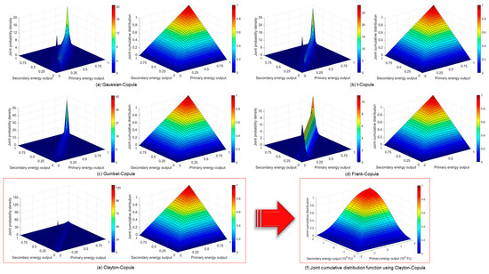
Figure 1.
Joint probability density and joint cumulative distribution under different Copula functions.

Table 1.
Values of parameters and evaluation metric for bivariate Copula functions.
3. Methodology and Modeling Formulation
3.1. Methodology
In energy and environment systems planning (EES) problems, extreme random uncertainties can be present as interactive random variables, and EES have dynamic characteristics. Thus, the decision scheme has to be developed under various probability levels. According to ref [30], Copula-based stochastic programming (CSP) has the advantages of reflecting uncertain interaction among random variables (existing in right-hand sides), particularly when the random variables have different probability distributions and previously unknown correlations. Combined with [31], CSP can be explained as follows:
Subject to
where f is linear objective function; xj are decision variables; cj and aij are parameters; are random variables; 1 − p is prescribed joint probability level; C denotes determinate Copula; pi are constraint violation levels of individual chance constraints; .
CSP has superiority in modeling joint distribution among random variables. Nevertheless, in the decision-making process, because of the influence of policy, economic, social, market, and technical factors, as well as incompleteness and inaccuracy, obtained data may have some errors. This can result in uncertainties in parameters, which fluctuate in a certain interval range. Interval linear programming (ILP) can tackle uncertainties presented as interval values. According to [32], ILP can be defined as follows:
Subject to
where , , , ; are interval numbers; are decision variables.
Therefore, techniques of CSP and ILP can be combined into a framework, leading to a Copula-based interval stochastic programming (CISP) model as
Subject to
However, in real-word EES planning, CISP is incapable of evaluating the costs and benefits of each scheme; it has difficulties in judging the relationship between investment and benefit to measure the value of each scheme. Cost–benefit analysis (CBA) provides a way to evaluate costs and benefits of various schemes so as to obtain the best scheme with the most benefit and the least cost in investment decision based on certain principles [33]. Specifically, CBA could compute net benefit through the cost and benefit of various schemes, as depicted as
where N is net benefit, B is general benefit, which includes total investing cost, Cz are costs of z type. CBA can evaluate the value of various schemes with the help of some indicators. Among them, the cost–benefit ratio can assess the feasibility of each scheme, while the net present value rate can evaluate profitability after implementation of a scheme. The value of cost–benefit ratio and net present value rate can be defined as follows:
where Ud are cost–benefit ratios of d scheme; Wd are net present value ratios of d scheme; Cdg are total costs of d scheme in g year; Bdg are total benefits of d scheme in g year; r is ratio of social discount, Id are original investment present values of d scheme.
Consequently, to tackle uncertainties expressed as intervals and interactive random variables, as well as evaluate the present value of costs and benefits to find the best scheme, CSP, ILP, and CBA methods could be integrated in a framework. Then, Copula-based interval cost–benefit stochastic programming (CICS) can be generated. The detailed solution process of CICS can be defined as follows:
- Step 1. Select optimal Copula function.
- Step 2. Formulate CICS through integrating CSP, ILP, and CBA methods.
- Step 3. On the basis of optimal Copula function, convert joint probability p into individual probabilities p1, p2, p3, …, pl.
- Step 4. Turn CICS into sub-models and .
- Step 5. Solve and to obtain decision variables and costs .
- Step 6. Calculate corresponding benefits and net benefits .
- Step 7. Obtain cost–benefit ratios and net present value rates of d scheme.
- Step 8. Stop.
3.2. CICS-EES Modeling Formulation
Based on the CICS method, a CICS-EES model is proposed for EES planning of Yulin City, a typical coal-dependent city in China (as shown in Figure 2). Before the CICS-EES model is formulated, three assumptions for the model should be explained: (1) primary energy includes coal, oil, and natural gas, and secondary energy includes coke, coke oven gas, electricity, and coal gangue; (2) primary energy output and secondary energy output are random variables with previously unknown probability distributions, and a joint cumulative distribution function is used for measuring their statistical dependence; and (3) based on “Ambient air quality standards” (GB 3095-2012), 3 types of pollutants are considered including SO2, NO2, and PM10. The planning horizon is 15 years (2022–2036), which is divided into 3 stages, with each being 5 years. A list of nomenclature in the CICS-EES model is presented in Appendix B.
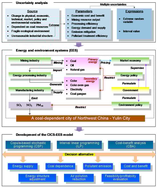
Figure 2.
Application framework of CICS-EES model in Yulin City.
- (1)
- Objective function. The objective of the model is to minimize system costs involving energy costs (), energy transportation costs (), industrial operational costs (), and pollutant treatment costs ().
- Energy costs. Energy costs refer to total energy purchase costs of the mining business, energy machining business, and manufacturing business.
- Energy transportation costs. Energy loss costs in transporting and utilization are contained in energy transportation costs.
- Industrial operational costs. Maintenance and depreciation cost of equipment, taxation cost, and workers’ wage are taken into account.
- Pollutant treatment costs. Pollutant treatment costs include pollutant treatment facilities costs, pollutant treatment system operating costs, and pollutant discharge costs.
- (2)
- Corresponding benefits () and net benefits () of each EAS planning scheme can be calculated.
- (3)
- Constraints include energy demand–supply balance, manufacturing business demand–supply balance, mass balance, as well as environment requirement.
- Energy demand–supply balance constraints. These constraints can guarantee that primary energy demand and secondary energy demand are met at a joint probability level.
- Manufacturing business demand–supply balance constraints. These constraints can guarantee that the product demands of the manufacturing business are satisfied.
- Mass balance constraints. The constraints ensure the energy utilization efficiency must be less than 1.
- Environment requirement constraints. The pollutant concentration should not be higher than the pollutant concentration standard specified in the ambient air quality standards.
- Nonnegative constrains.
3.3. Scenarios Construction
In this study, given the extreme dependence of energy consumption on coal resources, a number of scenarios (i.e., S1–S9 and S1′–S9′ of CSP; E1–E6 of coal reduction levels; T1–T9 of CCP) would be analyzed. Scenarios S1–S9 and S1′–S9′ of CSP are considered according to Clayton–Copula. Table 2 provides selected values of joint cumulative distribution , conditional cumulative distribution , and marginal cumulative distributions and , where X and Y are random variables representing primary energy output and secondary energy output, respectively.
Table 2.
Select values under scenarios S1–S9 of CSP.
Thereafter, constraint-violation levels (W, w1, w2) can be obtained, where (1 − W) is joint probability levels, and (1 − w1) and (1 − w2) are, respectively, individual probability levels corresponding to X and Y. By calculation of CICS-EES model under scenarios S1–S9, the scenario with the highest net present value ratio can be obtained. Then, six scenarios E1–E6 of coal reduction levels would be considered, according to the “Comprehensive work plan for energy conservation and emission reduction in ‘Thirteenth Five-Year Plan’ stage of Yulin City” [34].
Figure 3 illustrates the scenario tree of the study; scenarios E1–E6 of coal reduction levels would be associated with the scenario S in order to generate the best decision alternative. In addition, scenarios T1–T9 are designed based on CCP for comparison with scenarios S1′–S9′ of CSP.
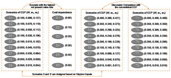
Figure 3.
Scenario tree of the study.
4. Results and Discussion
A CICS-EES model was developed and applied to EES planning in Northwest China, Yulin City, and then the best decision alternative was generated. By computing the model, scenario S1 with the highest net present value rate was selected and associated with coal reduction levels (i.e., E1–E6) for further analysis. The results showed that different constraint-violation levels and coal reduction levels would generate different energy supply schemes, which would lead to changes in pollutant emissions and system cost and benefit. Through the dependence degree evaluation of economic growth on coal under various schemes, the scheme with the lowest coal dependence index was provided for managers.
4.1. Uncertain Analysis
In this study, in order to reflect energy demand–supply risk, nine scenarios of joint and individual constraint-violation levels of violating energy demand in Yulin City were considered. Uncertainties related to different scenarios S1–S9 of CSP would result in different industrial energy supplies (as shown in Figure 4) and changed pollutant emissions (as shown in Figure 5).
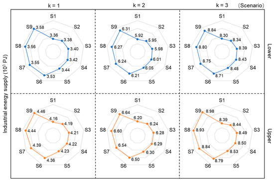
Figure 4.
Industrial energy supply under scenarios S1–S9 of CSP.
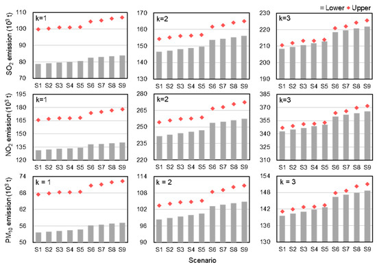
Figure 5.
Pollutant emission under scenarios S1–S9 of CSP.
Figure 5 shows pollutant emission under scenarios S1–S9 of CSP. From S1 to S9, the emission of each pollutant increases under the same planning stage k. For each pollutant, emissions also increase with the planning stage.
And then, varied system costs and net benefits are generated. Specifically, it can be obtained from Figure 6a,b that a higher joint constraint-violation level would lead to a lower system cost and a higher net benefit. This is because joint constraint-violation (W) levels indicate joint violation levels of not satisfying the energy output of whole EES, with a higher W level (i.e., a lower energy output) corresponding to a decreased industrial energy supply, which leads to a lower pollutant emission and system cost and then generates a higher net benefit; however, the system would confront the higher risk of industrial energy supply shortage. On the contrary, a lower W level (i.e., a higher energy output) corresponding to an increase in industrial energy supply, thus leading to a higher pollutant emission and system cost, would then generate a lower net benefit; but in this case, the system is incapable of withstanding changes in environmental policies. The results indicate that there is a tradeoff among industrial energy supply, pollutant emission, as well as system costs and net benefits. Additionally, through comparing various scenarios at the same W level, the results disclosed that the system cost shows a downward tendency, while net benefits show an upward one, with increased individual constraint-violation (w1 and w2) levels. The results of different w1 and w2 levels are not only effective for investigating the interactions of primary energy output and secondary energy output, as well as their effect on system cost and net benefit, but also in providing an approach for reaching equilibrium among energy demand–supply, pollutant emission control, and system cost and net benefit. In order to evaluate the feasibility and profitability that can be achieved of scenarios S1–S9, the cost–benefit ratio and net present value ratio are calculated in Figure 6c,d.
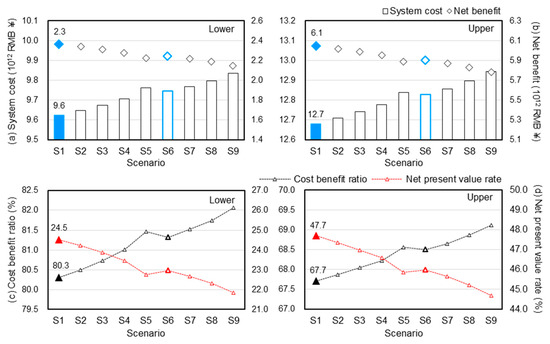
Figure 6.
Cost–benefit analysis under scenarios S1–S9 of CSP.
Figure 6c presents that the cost–benefit ratios are less than 100% of scenarios S1–S9, which indicates that the S1–S9 are all economically feasible. Generally, a higher net present value rate indicates a higher profitability of the scheme. It can be seen from Figure 6d that scenario S1 has the highest net present value rate (i.e., [47.7, 67.7] %). Therefore, scenario S1 was selected and associated with coal reduction levels (i.e., E1–E6) for generating the best scheme.
4.2. Coal Dependence Analysis
As the coal reduction levels change, the industrial energy supply structures would be different. Table 3 depicts industrial energy supply under scenarios E1–E6 of coal reduction levels.
Table 3.
Industrial energy supply under scenarios E1–E6 of coal reduction levels.
The results illustrate that industrial secondary energy support would display a downward trend while the coal reduction levels rise. The reason is that coke and coke oven gas are derived from deep processing of coal resources and coal gangue is a by-product of the coal mining process and coal washing process. A higher level of coal reduction corresponds to a lower level of coal mining and supply, and a lack of raw materials will lead to a reduction in coke, coke oven gas, and coal gangue output, which result in a decrease in industrial energy supply. Additionally, coal resources play a dominant role in the electricity production of EES in Yulin City, accounting for more than 90%. Therefore, industrial electricity supply would show a downward trend as coal reduction levels increase. Moreover, the increase in coal reduction levels would lead to an increase in industrial oil supply and a decrease in natural gas supply. This phenomenon is due to the higher exploitation and transportation cost of natural gas than that of oil. In each industrial energy supply scheme, the scheduling order depends on system cost, which is the scheme where a low energy supply cost is preferred. Figure 7 illustrates pollutant emissions (SO2, NO2 and PM10) of EES under different coal reduction levels. Generally, due to higher pollutant discharge and lower price, coal utilization is the leading source of pollutant emission for EES. The range of pollutant emissions decreases from stage 1 to 3, which is because the lower-bound energy supply growth rate is higher than the upper-bound with the increasing industrial energy demand.
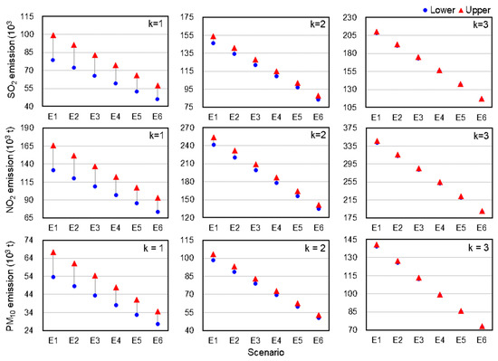
Figure 7.
Pollutant emission under scenarios E1–E6 of coal reduction levels.
Figure 8 provides the cost–benefit analysis under scenarios E1–E6 of coal reduction levels, which illustrates that a higher coal reduction level would lead to a lower cost–benefit ratio and a higher net present value ratio. The industrial structure of Yulin City is dominated by coal and related industries, which results in an extreme reliance on coal consumption for economic development. In order to quantitatively evaluate the dependence degree of economic growth on coal under different scenarios, the coal dependence index can be calculated (as shown in Appendix C). The values of parameters for the coal dependence index are listed in Table A2. In the schemes E1–E6 under the scenario of a coal reduction level, the coal dependence index shows complete dependence in the scheme of E1. In the schemes of E2, E3, E4, E5, and E6, they are [0.96, 0.97], [0.84, 0.85], [0.76, 0.78], [0.16, 0.17], and [0.27, 0.29], respectively. In the comparison of upper and lower-bound, the coal reduction level scheme E5 (that is, the reduction level of coal is 40%), when the coal dependency index is [0.16, 0.17], can achieve the lowest coal dependence index.
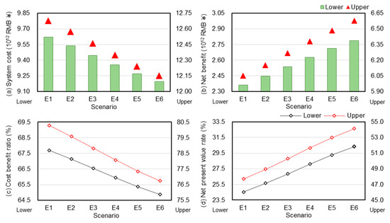
Figure 8.
Cost–benefit analysis under scenarios E1–E6 of coal reduction levels.
Therefore, by trading off system profitability and coal dependence index, scenario S1–E5 would be selected as the best decision alternative. Under S1–E5, decision makers are required to increase primary energy output by 9%, secondary energy output by 13%, and reduce industrial coal supply by 40%. In this case, the system cost would be RMB ¥ [9.27, 12.24] × 1012, net benefit would be RMB ¥ [2.71, 6.49] × 1012, corresponding cost–benefit ratio would be [65.4, 77.4] %, net present value rate would be [29.3, 53.0] %, and the coal dependence index would be [0.16, 0.17].
4.3. Comparative Analysis
To further illustrate the superiority of the CSP method for EES management, the study is turned into a chance-constrained programming (CCP) for comparison. A chance-constrained interval cost–benefit programming (CICC) (as shown in Appendix D) is formulated for planning EES, which leads to a CICC-EES model generated (as shown in Appendix E). Through solving the CICS-EES model under scenarios S1′–S9′ of the CSP and CICC-EES model under scenarios T1–T9 of CCP, the cost–benefit analysis can be obtained, as shown in Table 4.
Table 4.
Cost–benefit analysis under scenarios S1′–S9′ of CSP and T1–T9 of CCP.
Under all scenarios, the system costs from CICS-EES would range from RMB ¥ 9.11 × 10¹² to RMB ¥ 13.14 × 10¹²; correspondingly, the net present value rate would be from 31.51% to 42.54%. Meanwhile, the system costs would be from RMB ¥ 9.14 × 10¹² to RMB ¥ 13.23 × 10¹² and the net present value rate would be from 31.06% to 41.54% from CICC-EES.
Compared to CICC-EES, CICS-EES leads to lower system costs corresponding to higher net present value rates. This is because the objective of CICC-EES is to minimize system costs without considering the influence of joint constraint-violation of primary energy output and secondary energy output on the industrial energy supply structure of EES. Additionally, CICC-EES could merely tackle uncertainties represented as chances or probabilities, which neglect the correlations among random variables. In this case, it would cause a loss of uncertain information and a decrease in model reliability. The results reveal that the CICS-EES model incorporating the CSP method possesses a higher performance in uncertainty reflection, which is more economical for managers to plan EES in coal-dependent cities.
5. Conclusions
In this paper, a Copula-based interval cost–benefit stochastic programming (CICS) is proposed to handle extreme random uncertainties and support energy and EES planning of coal-dependent cities. The method proposed can reflect uncertainties shown as intervals or interactive random variables, as well as evaluate present costs and benefits. Then, the CICS-EES model is applied in planning EES of a typical coal-dependent city of China, Yulin City, during 2022–2036. Solutions of multiple scenarios under different constraint-violation levels and coal-reduction levels have been examined in the CICS-EES model. Some major findings can be summarized as follows: (i) with the increase in industrial energy supply constraint-violation level, system cost and pollutant emission would show a downward trend; (ii) by trading off system profitability and coal dependence index, scenario S1–E5 with the lowest coal dependence index was identified as the best decision alternative, in which decision makers are required to increase primary energy output by 9%, augment secondary energy output by 13%, and decrease industrial coal supply by 40%; corresponding to this, the system profitability could reach [29.3, 53.0] %; and (iii) compared with the CCP and CSP methods, CSP can address more inherent uncertainties and achieve a higher marginal net present value rate (i.e., [0.45, 1.00] %). Summarily, the results illustrate that the CICS-EES model can deal with inherent extreme random uncertainties, gain insight into the tradeoff between system reliability and profitability, and obtain overall satisfactory EES planning schemes. results also display that the developed model shows flexibility, which is able to be extended to EES planning of other similar coal-dependent cities for optimizing energy structures, improving industrial energy supply efficiency, reducing pollutant emissions, and enhancing system profitability.
Author Contributions
Conceptualization, Y.Z. and Y.L. (Yanzheng Liu); methodology, Y.Z.; software, Z.W.; validation, Z.W., J.T. and S.C.; formal analysis, Y.L. (Yanzheng Liu); investigation, Y.G.; resources, Z.W.; data curation, Z.W.; writing—original draft preparation, Z.W.; writing—review and editing, Z.W. and J.T.; visualization, Y.L. (Yexin Li) and S.L.; supervision, Y.Z.; project administration, Y.Z.; funding acquisition, Y.Z. All authors have read and agreed to the published version of the manuscript.
Funding
This research was funded by NATIONAL KEY RESEARCH PROJECTS, grant number 2016YFC0207800, NATIONAL NATURAL SCIENCE FOUNDATION OF CHINA, grant number 51809145, UNDERGRADUATE TRAINING PROGRAM FOR INNOVATION AND ENTREPRENEURSHIP OF SHAANXI PROVINCE, grant number S202310703, and SHAANXI PROVINCIAL KEY PROGRAM FOR SCIENCE AND TECHNOLOGY DEVELOPMENT, grant number 2022KWZ-25.
Institutional Review Board Statement
Not applicable.
Informed Consent Statement
Not applicable.
Data Availability Statement
The data used to support the findings of this study can be made available by the corresponding author upon request.
Acknowledgments
The authors are deeply grateful to the editors and the anonymous reviewers for their insightful comments and helpful suggestions, which have greatly helped improve the manuscript.
Conflicts of Interest
Authors Mr. Yexin Li and Mr. Yong Guo were employed by Ankang Environmental Engineering Design Limited Company. The remaining authors declare that the research was conducted in the absence of any commercial or financial relationships that could be construed as a potential conflict of interest..
Appendix A. Coal Dependence Index
The coal dependence index is an indicator that quantitatively evaluates the dependence degree of economic growth on coal. It can be defined as follows:
where Ic are coal dependence indexes; Ci are individual evaluation indexes of i type; Wi are weights of i type individual evaluation index. Among them, individual evaluation index Ci is calculated as follows:
where Cdi are i type individual evaluation indexes of d scheme; Cbi are reference values of i type individual evaluation indexes. Significantly, the coal dependence index would deviate from the actual situation when the individual evaluation index and the reference value are quite different. Therefore, the unreasonable influence can be amended as follows:
In this study, 2010 was selected as the reference value of individual evaluation index. Table A1 presents the values of parameters for the coal dependence index of Yulin City and the Chinese average.

Figure A1.
Coal dependence index of Yulin City and Chinese average since 2010.
Table A1.
Values of parameters for coal dependence index in Yulin City and China.
Table A1.
Values of parameters for coal dependence index in Yulin City and China.
| Individual Evaluation Index | Unit | Weight | Reference Value | |
|---|---|---|---|---|
| Yulin City | China | |||
| The proportion of industrial coal supply in energy supply | % | 30 | 0.88 | 0.68 |
| Contribution rate of industrial coal supply to energy supply growth | % | 30 | 0.98 | 0.92 |
| Coal consumption coefficient per unit GDP | t/109 RMB ¥ | 40 | 17,240.07 | 0.60 |
Appendix B. List of Abbreviations and Symbols
Appendix B.1. Abbreviations
| CCP | Chance-constrained programming |
| CICC | Chance-constrained interval cost–benefit programming |
| CICS | Copula-based interval cost–benefit stochastic programming |
| CBA | Cost–benefit analysis |
| CSP | Copula-based stochastic programming |
| EES | Energy and environment systems |
| ILP | Interval linear programming |
| SMP | Stochastic mathematical programming |
Appendix B.2. Symbols
| type of manufacturing business, i = 1 means chemical materials and manufacturing business, i = 2 means non-metallic mineral products business, i = 3 means ferrous metal smelting and machining business, i = 4 means non-ferrous metal smelting and machining business. | |
| pollutant type, j = 1 means SO2, j = 2 means NO2, j = 3 means PM10. | |
| planning stage, k = 1 means 2021–2025, k = 2 means 2026–2030, k = 3 means 2031–2035. | |
| mining business type, m = 1 means coal mining and washing business, m = 2 means oil and gas business, m = 3 means metal mining business, m = 4 means non-metallic mining business. | |
| energy machining business type, o = 1 means petroleum machining, coking, business, o = 2 means electricity and heat production-supply business. | |
| primary energy type, p = 1 means coal, p = 2 means oil, p = 3 means natural gas. | |
| secondary energy type, s = 1 means coke, s = 2 means coke oven gas, s = 3 means electricity, s = 4 means coal gangue. | |
| disbursements of pollutant treatment in manufacturing business i in stage k. | |
| disbursements of pollutant treatment in energy machining business o in stage k. | |
| unit prices for primary energy p in stage k. | |
| unit prices for secondary energy s in stage k. | |
| expected disbursements of system. | |
| average effective stack height. | |
| energy consumption factors of unit output on manufacturing business i in stage k. | |
| investment disbursements of pollutant handling equipment on manufacturing business i in stage k. | |
| investment disbursements of pollutant handling equipment of energy machining business o in stage k. | |
| operation disbursements of producing unit product of manufacturing business i in stage k. | |
| product outputs of manufacturing business i in stage k. | |
| market prices of manufacturing business i in stage k. | |
| emission factors from primary energy p to pollutant j in stage k. | |
| emission factors from secondary energy s to pollutant j in stage k. | |
| disposal disbursements on unit pollutant j in stage k | |
| efficiency disbursements on pollutant discharge of pollutant j. | |
| pollutant emission rates of pollutant j of manufacturing business i in stage k. | |
| pollutant concentration standards of pollutant j in stage k. | |
| treatment efficiencies of pollutant j. | |
| efficiency equivalent values of pollutant j. | |
| loss disbursements of primary energy p in stage k. | |
| loss disbursements of secondary energy s in stage k. | |
| mining disbursements of unit primary energy p in stage k. | |
| the amount of businesses exceeding scale of manufacturing business i in stage k. | |
| the amount of businesses exceeding scale of energy machining business o in stage k. | |
| product demands of manufacturing business i in stage k. | |
| general exportations of primary energy p in stage k. | |
| general exportations of secondary energy s in stage k. | |
| conversion factors from primary energy p towards standard coal. | |
| supply quantity, primary energy p on manufacturing business i in stage k. | |
| supply quantity, primary energy p on mining business m in stage k. | |
| supply quantity, primary energy p on energy machining business o in stage k. | |
| transmission disbursements on primary energy p in stage k. | |
| conversion factors from secondary energy s towards standard coal. | |
| supply quantity on secondary energy s of manufacturing business I in stage k. | |
| supply quantity on secondary energy s of mining business m in stage k. | |
| supply quantity on secondary energy s of energy machining business o in stage k. | |
| machining disbursements on unit mass secondary energy s in stage k. | |
| transmission disburse on secondary energy s in stage k. | |
| wind velocity. | |
| prescribed joint constraint-violations. | |
| individual constraint-violations corresponding to primary energy output. | |
| individual constraint-violations corresponding to secondary energy output. | |
| plume standard deviations in direction y. | |
| plume standard deviations in direction z. |
Appendix C. Values of Parameters for Coal Dependence Index
In this study, scenario E1 of coal reduction level was selected as the reference value of individual evaluation index. Table A2 shows the values of parameters for coal dependence index.
Table A2.
Interval values of parameters for coal dependence index.
Table A2.
Interval values of parameters for coal dependence index.
| Individual Evaluation Index | Unit | Weight | Reference Value |
|---|---|---|---|
| The proportion of industrial coal supply in energy supply | % | 30 | [0.80, 0.81] |
| Contribution rate of industrial coal supply to energy supply growth | % | 30 | [0.25, 0.60] |
| Coal consumption coefficient per unit net benefit generated | kg/RMB ¥ | 40 | [3872.70, 4068.10] |
Appendix D. Chance-Constrained Interval Cost–Benefit Programming (CICC)
Chance-constrained programming (CCP) is widely used to deal with uncertainties in parameters, which can be represented as chances or probabilities [35]. CCP can be expressed as follows:
Subject to
where f is objective function; xj are decision variables; aij, bi, and cj are parameters; are random variables; pi are constraint-violation levels. Then, the constraint can be converted into an equivalent constraint [31]:
where , given the cumulative distribution function of .
A chance-constrained interval programming (CICP) method, which integrates CCP and ILP can be proposed as follows:
Subject to
Then, a chance-constrained interval cost–benefit programming (CICC) method through incorporating techniques of CICP and CBA with a framework to handle uncertainties expressed as random variables and intervals, as well as cost–benefit analysis.
Appendix E. CICC-EES Modeling Formulation
Through integrating the CICC method into the EES system, a CICC-EES model is formulated as follows:
- (1)
- Objective function.
- Energy costs.
- Energy transportation costs.
- Industrial operational costs.
- Pollutant treatment costs.
- (2)
- Corresponding benefits () and net benefits () of each EAS planning scheme.
- (3)
- Constraints.
- Energy demand–supply balance constraints.
- Manufacturing business demand–supply balance constraints.
- Mass balance constraints.
- Environment requirement constraints.
- Nonnegative constraints.
References
- Ren, F.; Yu, X. Coupling analysis of urbanization and ecological total factor energy efficiency—A case study from Hebei province in China. Sustain. Cities Soc. 2021, 74, 103183. [Google Scholar] [CrossRef]
- Zhu, Y.; Wei, Z.; Li, Y.X.; Du, H.X.; Guo, Y. Energy and atmosphere system planning of coal-dependent cities based on an interval minimax-regret coupled joint-probabilistic cost-benefit approach. Energy 2022, 239, 122154. [Google Scholar] [CrossRef]
- The State Council of the People’s Republic of China. National Plan for Sustainable Development of Resource-Dependent Cities (2013–2020). 2013. Available online: http://www.gov.cn/zwgk/2013-12/03/content_2540070.htm (accessed on 1 November 2020).
- Han, J.Z.; Hu, Z.Q.; Wang, P.J.; Yan, Z.G.; Li, G.S.; Zhang, Y.H.; Zhou, T. Spatio-temporal evolution and optimization analysis of ecosystem service value-A case study of coal resource-based city group in Shandong, China. J. Clean. Prod. 2022, 363, 132602. [Google Scholar] [CrossRef]
- Wang, D.; Ji, X.; Li, C.; Gong, Y. Spatiotemporal Variations of Landscape Ecological Risks in a Resource-Based City under Transformation. Sustainability 2021, 13, 5297. [Google Scholar] [CrossRef]
- Guan, P.B.; Huang, G.H.; Wu, C.B.; Wang, L.R.; Li, C.C.; Wang, Y.Y. Analysis of emission taxes levying on regional electric power structure adjustment with an inexact optimization model—A case study of Zibo, China. Energy Econ. 2019, 84, 104485. [Google Scholar] [CrossRef]
- Asif, Z.; Chen, Z. A life cycle-based air quality modeling and decision support system (LCAQMS) for sustainable mining management. J. Environ. Inform. 2020, 35, 103–117. [Google Scholar] [CrossRef]
- Zheng, H.T.; Zheng, L.; Ni, W.D.; Larson, E.D.; Ren, T.J. Case-study of a coal gasification-based energy supply system for China. Energy Stustain. Dev. 2003, 7, 63–78. [Google Scholar] [CrossRef]
- Roch, I. Brown coal planning as a basis for sustainable settlement development. Earth Planet. Sci. Lett. 2009, 1, 857–867. [Google Scholar] [CrossRef][Green Version]
- Li, H.; Dong, L.; Ren, J.Z. Industrial symbiosis as a countermeasure for resource dependent city: A case study of Guiyang, China. J. Clean. Prod. 2015, 107, 252–266. [Google Scholar] [CrossRef]
- Campbell, M.; Nel, V.; Mphambukeli, T. A thriving coal mining city in crisis? The governance and spatial planning challenges at Witbank, South Africa. Land Use Pol. 2017, 62, 223–231. [Google Scholar] [CrossRef]
- Tai, X.L.; Xiao, W.; Tang, Y.X. A quantitative assessment of vulnerability using social-economic-natural compound ecosystem framework in coal mining cities. J. Clean. Prod. 2020, 258, 120969. [Google Scholar] [CrossRef]
- Jin, S.W.; Li, Y.P.; Yu, L.; Suo, C.; Zhang, K. Multidivisional planning model for energy, water and environment considering synergies, trade-offs and uncertainty. J. Clean. Prod. 2020, 259, 121070. [Google Scholar] [CrossRef]
- Kung, C.C.; Wu, T. Influence of water allocation on bioenergy production under climate change: A stochastic mathematical programming approach. Energy 2021, 231, 120955. [Google Scholar] [CrossRef]
- Suo, C.; Li, Y.P.; Sun, J.; Yin, S. An air quality index-based multistage type-2-fuzzy interval-stochastic programming model for energy and environmental systems management under multiple uncertainties. Environ. Res. 2018, 167, 98–114. [Google Scholar] [CrossRef] [PubMed]
- Yu, L.; Xiao, Y.; Jiang, S.; Li, Y.P.; Fan, Y.R.; Huang, G.H.; Lv, J.; Zuo, Q.T.; Wang, F.Q. A copula-based fuzzy interval-random programming approach for planning water-energy nexus system under uncertainty. Energy 2020, 196, 117063. [Google Scholar] [CrossRef]
- Sklar, A. Fonctions de Répartition à n Dimensions Etleursmarges; Publications de l’Institut de Statistique de l’Université de Paris: Paris, France, 1959; Volume 8, pp. 229–231. [Google Scholar]
- Zhang, Y.F.; Li, Y.P.; Huang, G.H.; Ma, Y. A copula-based stochastic fractional programming method for optimizing water-food-energy nexus system under uncertainty in the Aral Sea basin. J. Clean. Prod. 2020, 292, 126037. [Google Scholar] [CrossRef]
- Suo, C.; Li, Y.P.; Nie, S.; Lv, J.; Mei, H.; Ma, Y. Analyzing the effects of economic development on the transition to cleaner production of China’s energy system under uncertainty. J. Clean. Prod. 2021, 279, 123725. [Google Scholar] [CrossRef]
- Kouaissah, N.; Hocine, A. Optimizing sustainable and renewable energy portfolios using a fuzzy interval goal programming approach. Comput. Ind. Eng. 2020, 144, 106448. [Google Scholar] [CrossRef]
- Chen, C.; Yu, L.; Zeng, X.; Huang, G.; Li, Y. Planning an Energy–Water–Environment Nexus System in Coal-Dependent Regions under Uncertainties. Energies 2020, 13, 208. [Google Scholar] [CrossRef]
- Li, Y.; Feng, B.; Wang, B.; Sun, S.C. Joint planning of distributed generations and energy storage in active distribution networks: A Bi-Level programming approach. Energy 2022, 245, 123226. [Google Scholar] [CrossRef]
- Li, W.S.; Zhao, L.; Bo, Y.; Wang, W.L.; Wang, M.Q.; Liu, S.; Liu, R.; Wang, X. Robust transmission expansion planning model considering multiple uncertainties and active load. Glob. Energy Interconnect. 2021, 4, 476–484. [Google Scholar] [CrossRef]
- Wu, J.; Wu, N.; Feng, Q.; Deng, C.; Zhang, X.; Fu, Z.; Zhang, Z.; Li, H. Design and Optimization of a Coal Substitution Path Based on Cost–Benefit Analysis: Evidence from Coal Resource-Based Cities in China. Sustainability 2023, 15, 15448. [Google Scholar] [CrossRef]
- Barić, D.; Grabušić, S.; Jakara, M.; Emanović, M. Reviewing the Cost–Benefit Analysis and Multi-Criteria Decision-Making Methods for Evaluating the Effectiveness of Lithium-Ion Batteries in Electric Vehicles. Sustainability 2024, 16, 233. [Google Scholar] [CrossRef]
- Ministry of Ecology and Environment of the People’s Republic of China. Outline of the National Protection Plan for Ecologically Fragile Areas [EB/OL]. (2008-09-27). Available online: https://www.gov.cn/govweb/gzdt/att/att/site1/20081009/00123f37b41e0a57e2e601.pdf (accessed on 28 December 2023).
- Otsu, T.; Taniguchi, G. Kolmogorov-Smirnov type test for generated variables. Econ. Lett. 2020, 195, 109401. [Google Scholar] [CrossRef]
- Baak, M.; Koopman, R.; Snoek, H.; Klous, S. A new correlation coefficient between categorical, ordinal and interval variables with Pearson characteristics. Comput. Stat. Data Anal. 2020, 152, 107043. [Google Scholar] [CrossRef]
- Wang, D.; Fan, Q.; Ma, Y. An interactive maximum likelihood estimation method for multivariable Hammerstein systems. J. Franklin Inst. 2020, 357, 12986–13005. [Google Scholar] [CrossRef]
- Yu, L.; Li, Y.P.; Huang, G.H.; Fan, Y.R.; Yin, S. Planning regional-scale electric power systems under uncertainty: A case study of Jing-Jin-Ji region, China. Appl. Energy 2018, 212, 834–849. [Google Scholar] [CrossRef]
- Chen, F.; Huang, G.H.; Fan, Y.R.; Wang, S. A copula-based chance-constrained waste management planning method: An application to the city of Regina, Saskatchewan, Canada. J. Air Waste Manag. Assoc. 2017, 66, 307–328. [Google Scholar] [CrossRef]
- Huang, G.H.; Baetz, B.W.; Patry, G.G. Grey integer programming: An application to waste management planning under uncertainty. Eur. J. Oper. Res. 1995, 83, 594–620. [Google Scholar] [CrossRef]
- Cabrales, S.; Valencia, C.; Ramírez, C.; Ramírez, A.; Herrera, J.; Cadena, A. Stochastic cost-benefit analysis to assess new infrastructure to improve the reliability of the natural gas supply. Energy 2022, 246, 123421. [Google Scholar] [CrossRef]
- The People’s Government of Yulin City. Comprehensive Work Plan for Energy Conservation and Emission Reduction in “Thirteenth Five-Year Plan” Stage of Yulin City 2018. Available online: http://www.yl.gov.cn/P/C/34072.htm (accessed on 1 November 2020).
- Yu, L.; Li, Y.P.; Huang, G.H.; Shan, B.G. A hybrid fuzzy-stochastic technique for planning peak electricity management under multiple uncertainties. Eng. Appl. Artif. Intel. 2017, 62, 252–264. [Google Scholar] [CrossRef]
Disclaimer/Publisher’s Note: The statements, opinions and data contained in all publications are solely those of the individual author(s) and contributor(s) and not of MDPI and/or the editor(s). MDPI and/or the editor(s) disclaim responsibility for any injury to people or property resulting from any ideas, methods, instructions or products referred to in the content. |
© 2024 by the authors. Licensee MDPI, Basel, Switzerland. This article is an open access article distributed under the terms and conditions of the Creative Commons Attribution (CC BY) license (https://creativecommons.org/licenses/by/4.0/).