Understanding the Determinants of Lane Inefficiency at Fully Actuated Intersections: An Empirical Analysis

Abstract

As urban traffic challenges intensify, the growing interest for fully actuated control systems in intersection management is on the rise due to their capacity to adapt to dynamic traffic demands. These systems play a crucial role in sustainable traffic solutions, significantly reducing delays and emissions and enhancing overall system efficiency. The optimal performance of these systems relies on effectively facilitating vehicle discharge at the saturation flow rate throughout the green period. This study introduces a new parameter, lane inefficiency, evaluating vehicle discharge effectiveness by comparing saturation flow rate with instantaneous discharge for each green period. It provides a comprehensive assessment of green utilization for specific lanes. This study also explores the impact of signal control system parameters and traffic flow characteristics on lane inefficiency using principal component analysis (PCA) and multiple linear regression models. This approach holistically evaluates how both signal control system and traffic flow parameters collectively influence efficient green period utilization. The findings emphasize the impact of critical factors on lane inefficiency, including green time, the proportion of total unused green time to green time, total unused green time, the percentage of heavy vehicles in departing traffic, the ratio of effective green time to cycle time, the total time headways of the first four vehicles, and queue length. Decision makers need to pay due attention to these parameters to enhance intersection performance and foster a more sustainable urban transportation network.

1. Introduction

The escalating urban population has fueled a notable surge in traffic congestion in urban areas, making traffic management a critical issue [1]. At the heart of urban transportation networks, intersections have a pivotal influence on the overall efficiency of the road system [2]. Among the strategies employed to manage intersections, traffic signal control stands out, particularly in densely populated and well-developed urban road networks [3].

It is imperative to underscore that well-managed intersections are not only instrumental in enhancing traffic flow but also have a significant influence on advancing urban sustainability objectives. Well-managed intersectional practices result in increased capacity, mitigating traffic congestion and consequently reducing emissions, aligning seamlessly with sustainability principles [4]. This emphasizes the crucial role of adopting traffic management practices that not only optimize vehicular movement but also substantially contribute to broader environmental goals. Traditionally, fixed-time systems have been the go-to for managing urban intersections, assigning pre-defined green times under the assumption of steady traffic flow. However, this assumption often falters in practice, given the fluctuating nature of traffic flow rates throughout the day and week [5]. In response to the dynamic nature of traffic demand, the surge in popularity of fully actuated control systems is notable. Fully actuated signal control is a concept wherein vehicular traffic data are detected in real time from all intersection approach legs via sensors, and these data are evaluated simultaneously via an algorithm that aims to minimize the delay or queue from all approach legs and maximize the number of vehicles passing through the intersection in one cycle. These systems dynamically adjust cycle lengths, green time allocations, and phase sequences in real-time based on arrival flow rates [6,7]. This adaptive approach not only optimizes traffic efficiency but also, crucially, aligns with sustainability goals by responding in real time to traffic conditions, thereby contributing substantially to reductions in the overall environmental footprint [8,9].

At the heart of maximizing intersection capacity lies the saturation flow rate, a pivotal parameter in traffic signal system planning and design [10]. Beyond its technical significance, the saturation flow rate intertwines with sustainability by influencing traffic signal system planning and design, which are integral to achieving sustainable urban mobility. Vehicles discharge at the saturation flow rate until the queue dissipates, a period called queue service time [11]. The green extension period following the discharge of queued vehicles plays a pivotal role in determining the effectiveness of signal control. The optimal performance of signal control systems hinges on their ability to facilitate vehicle discharges at the saturation flow rate during the green extension period.

Morozov et al. [12] argue that the traffic flow rate parameter alone is not sufficient for the efficient management of signal-controlled urban intersections. They developed a method for adjusting cycle time that examines changes in traffic flow rates at urban intersections, considering the impact of lane occupancy. Similarly, this study introduces a lane inefficiency parameter to gain insights into how efficiently vehicles are discharged at the saturation flow rate during the green period at intersections controlled by fully actuated signal systems. The lane inefficiency parameter, calculated by comparing the saturation flow rate with the instant discharge rate for each green period, offers a comprehensive evaluation of green utilization for specific lanes, constituting the main contribution of this research. It should be noted that given the fluctuation in green time for each signal cycle in fully actuated control systems, the saturation flow rate was recalculated for each green period. Furthermore, this study delves into the impact of signal control system parameters (e.g., green time, red time, and cycle time) and traffic flow parameters (e.g., queue length, departure flow, and vehicle composition) on lane inefficiency using PCA and multiple linear regression models. This detailed method not only helps us to discuss managing traffic in a technical manner but also expands our discussion to reveal how signal control systems and traffic patterns together affect the sustainable use of green traffic signals.

The rest of this article is structured as follows: First, a brief review of the related literature is presented. Second, the data collection process is introduced. Third, the methodology is described in detail. Fourth, the modeling results are presented. Finally, the conclusions are summarized along with further recommendations.

2. Literature Review

Leitner et al. [13] presented a literature review on the evaluation metrics employed for assessing signalized intersection performance. These performance indicators encompass a range of factors, including the green and red phase occupancy ratio [14], the platoon ratio [15], approach capacity [16], approach speed [17,18], congestion [19], travel time [20], peak hour volume, and delay [21].

The Highway Capacity Manual (HCM) 2010 [22] employs the volume-to-capacity ratio for evaluating performance at signalized intersections. The discharge flow rate and saturation flow rate are two significant parameters that have a close relationship with intersection volume and capacity. Time headway is a significant microscopic parameter used to accurately estimate the discharge flow rate at signalized intersections [23,24]. It is the time difference between successive vehicles passing the stop line at a signalized intersection and is inversely proportional to the discharge flow rate. Several researchers have studied discharge flow characteristics [25]. Li and Prevedouros [26] noted that the discharge rate increases in a straight lane, reaching its maximum value for between 9 and 12 vehicles. In the study by Denney et al. [27], it is suggested that long green times adversely affect the discharge rate. Li and Prevedouros [26] observed a decrease in the discharge rate after the 40th second of green time, while Khosla and Williams [28] suggested that this decline begins after the 60th second. Queue length is another parameter affecting the discharge rate, as found by Lin and Thomas [29], who discovered that an increase in queue length enhances the discharge rate. Conversely, Gao and Alam [30] indicated a decreasing trend in the discharge rate with an increasing queue.

The saturation flow rate holds significance in geometric design, signal control, and level-of-service evaluations at signalized intersections [31]. Numerous studies have delved into factors influencing the saturation flow rate. These factors encompass intersection geometry [32], grade [33], lane width and markings [34,35], vehicle composition [36], left- and right-turning vehicles [37], pedestrian and bicycle activity [38], signal characteristics [39], weather conditions [40], signal countdown devices [41] and autonomous vehicles [31]. In addition, it has been reported that the saturation flow rate is affected by drivers’ lane-changing behavior as they approach an intersection [38,42,43].

The conclusion drawn from existing research suggests that while numerous studies have delved into the performance of signal-controlled intersections, there exists a limited body of research exploring fluctuations in saturated flow, specifically at fully actuated intersections. Typically, the volume-to-capacity ratio or degree of saturation serves as a standard measure for evaluating the efficacy of signalized intersections. This metric calculates the hourly volume-to-capacity ratio for each phase of a signal system, assuming a macro-level perspective wherein green and cycle times remain constant. However, real-time-managed intersections strive to maintain the saturation flow rate during the green period, introducing variability in green times across signal cycles. Consequently, a micro-level approach that considers the fluctuation in green times and the instantaneous discharge rate within the green period becomes imperative for accurate performance evaluation, serving as the primary impetus behind this study. Furthermore, our objective is to enrich the literature by elucidating the factors influencing lane inefficiency through the application of mathematical models.

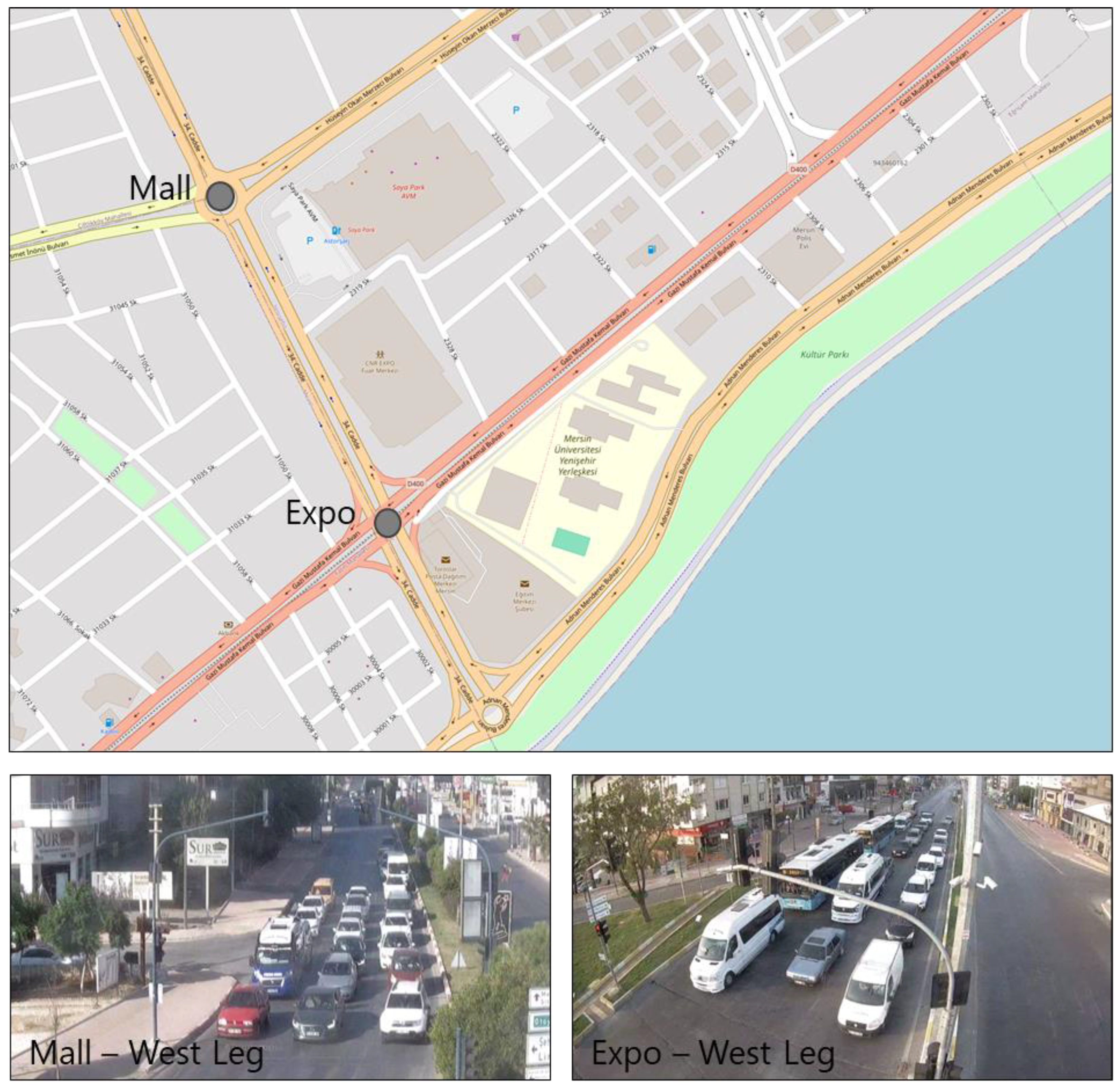
3. Study Area and Data Collection

Traffic flow data were collected for two isolated intersections in Mersin, Turkey: Expo Intersection, a four-way intersection, and Mall Intersection, a roundabout (see Figure 1). Both intersections have three lanes for each approach, and traffic in the middle lanes is slightly affected by vehicles turning left or right. The other attributes of these intersections are listed below:

• The lane widths range from 3 to 3.6 m;
• The approach slopes are negligible (i.e., less than 2%);
• Pedestrian activities are limited.

Traffic video recordings of the approach lanes were obtained from the Transportation Department of the Mersin Metropolitan Municipality. The recordings were captured during the morning peak hours on two weekdays, from 7:30 to 9:30 a.m., under dry and clear weather conditions. Signal system data, including the start and end times of the green and red periods for each signal cycle, were also acquired. Considerably high traffic volumes were observed for the West, East, and North approaches of the Mall Intersection and for the West approach of the Expo Intersection.

Table 1. Observed traffic volumes during the study period.

Day 1
Intersection	Approach	07:30–08:30			08:30–09:30
		Left	Middle	Right	Left	Middle	Right
Mall	West	545	1540	884	532	1512	942
	East	141	1103	878	125	1089	849
	North	358	557	211	372	449	241
Expo	West	765	998	201	689	801	199
Day 2
Intersection	Approach	07:30–08:30			08:30–09:30
		Left	Middle	Right	Left	Middle	Right
Mall	West	548	1467	991	572	1352	901
	East	114	1104	792	164	1210	756
	North	233	641	239	227	583	217
Expo	West	518	1020	149	573	1259	132

presents the observed traffic volumes for these approaches during the study period. Approaches with low traffic volumes were excluded from the study. Notably, these intersections can be considered isolated due to the low traffic volumes observed in the section between them and because of the absence of any formed queues.

4. Methodology

4.1. Concept of Lane Inefficiency

Figure 2 displays the instant discharge flow rates of vehicles during two observed green periods (G₁ = 36 s and G₂ = 38 s), both characterized by an identical saturation flow rate of 0.480 veh/s/lane (1728 veh/h/lane) and a consistent number of queued vehicles, which, in this case, is 11. Note that apart from the studies in the literature that provide saturation flow rate values in pcu/h/lane [44,45,46,47], there are also those presenting these values as vehicle/h/lane [38,48,49]. Therefore, in this study, the saturation flow rate was calculated as vehicles per hour per lane using the time headways of the vehicles. Then, the effect of heavy vehicles on lane efficiency was explored through developed models in Section 5.2.

In both instances depicted in Figure 2, it is evident that saturation flow was not achieved immediately after the initiation of the green signal. However, in the first scenario, saturation flow was attained starting from the third vehicle, while in the second scenario, it was achieved with the fifth vehicle. Upon closer examination, it becomes apparent that during the first green period, vehicles were discharged at or near the saturation flow. However, the same level of efficiency was not sustained during the second green period. Specifically, it was observed that saturation flow could not be maintained in the latter part of the 38 s green duration, approximately occurring after the 25th second. In this case, a significant portion of the green time was utilized efficiently. Therefore, assessments based solely on saturation flow would be insufficient. The necessity for a more detailed examination is apparent.

The identification of factors influencing this situation is deemed crucial for the optimization of intersection capacity, constituting the primary focus of this study. The lane inefficiency parameter (δ) was developed to derive insights into the effectiveness of vehicle discharge at saturation flow during the green period by comparing instant discharge rates with the saturation flow rate. Subsequently, an exploration into how lane inefficiency is influenced by signal control system parameters and traffic flow parameters, aiming for a comprehensive understanding of the factors contributing to the observed variations, was conducted.

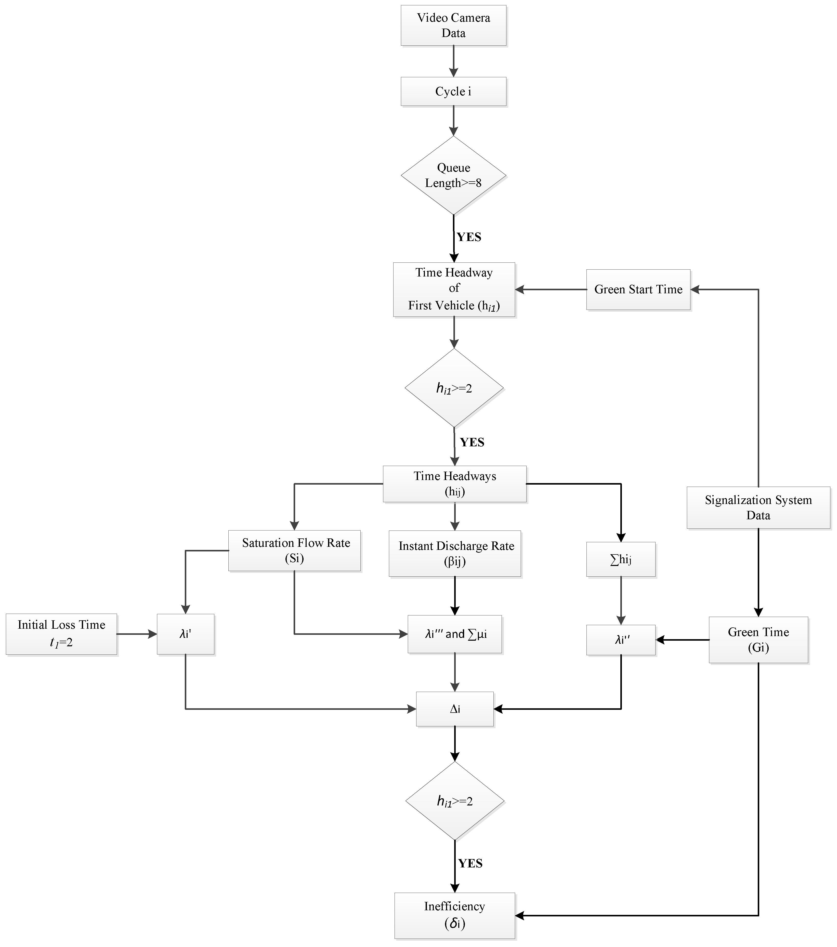
4.2. Calculation of the Lane Inefficiency

Previous studies indicated that the presence of vehicles making left and right turns negatively impacts the saturation flow rate and capacity of signalized intersections [37,50]. To minimize the impact of these vehicles on the saturation flow rate, only the middle lanes of intersection approaches were considered. A flowchart of the proposed methodology is presented in Figure 3. Saturation flow rate was calculated using the method described in Highway Capacity Manual 2010. HCM 2010 recommends that there should be at least eight vehicles in a standing queue to achieve saturation flow [22]. Consequently, at the start of each green period, video recordings were paused to ascertain the number of vehicles in the queue (see Figure 1). Only the green periods where there were at least eight vehicles in the queue were considered. The time headways between consecutive vehicles during each green period were determined by decoding the video images using MATLAB 2019b software. HCM 2010 recommends a value of 2 s for the initial loss time (t₁) [22]. Thus, green periods in which the time headway of the first vehicle was less than 2 s were excluded from the analysis (see Figure 3).

As an example, Figure 4 displays the saturation flow rate (S_i) (veh/s) for the green period i [22].

$$S_i=1/{hs}_i$$

(1)

Here, ${hs}_i$ refers to the saturated headway (s/veh) for the green period i. The saturated headway was calculated using Equation (2), where n refers to the total number of vehicles in a queue of green period i, and h_q refers to the time of qth queued vehicle in cycle i (s) [22].

$${hs}_i=\left({\sum }_{q=5}^n{h}_{iq}\right)/(n-4)$$

(2)

Figure 4 also displays the instant discharge rate (β_ij) during the green period i [22].

$${\beta }_{ij}=1/h_{ij}$$

(3)

Here, h_ij refers to the time headway of the jth vehicle that traverses the stop line during the green period i.

As depicted in Figure 4, the instant discharge rate fluctuates during the green period, which leads to inefficiency when it drops below the saturation flow rate. The total inefficiency consists of the following three components: (a) the inefficiency resulting from the initial unused green time (λ′), (b) the inefficiency resulting from the unused green time after the last vehicle passes the stop line (λ″), and (c) the sum of inefficiency resulting from the low instant discharge rate ($\sum \lambda ‴$). The total inefficiency is equal to

$${\lambda }_i={\lambda }_i^{\prime }+{\lambda }_i^{″}+\sum {\lambda }_i^{‴}$$

(4)

λ′ was calculated using Equation (5).

$${\lambda }_i^{\prime }={\theta }_i^{\prime }{S}_i$$

(5)

Here, ${\theta }^{\prime }$ refers to the initial unused green time (s) for the green period $i \mathrm{a}\mathrm{n}\mathrm{d}$ was calculated using Equation (6).

$${\theta }_i^{\prime }=h_{i1}-t_1$$

(6)

where $h_{\mathrm{i}1}$ refers to the time headway of the first vehicle in the queue. $t_1$ refers to the initial loss time, set at 2 s in line with the recommendations from the HCM 2010 [22]. The inefficiency resulting from the unused green time after the last vehicle (λ″) was calculated using Equation (7).

$${\lambda }_i^{″}={\theta }_i^{″}{S}_i$$

(7)

Above, ${\theta }^{″}$ refers to the unused green time after the last vehicle (s)

$${\theta }_i^{″}=G_i-{\sum }_{j=1}^m{h}_j$$

(8)

where G refers to the green time (s), and m is the departure volume for the green period i (i.e., the total number of vehicles traversing the stop line during the green period).

The sum of inefficiency resulting from the low instant discharge rate ($\sum {\lambda }^{‴}$) was calculated using an algorithm developed in MATLAB^®.

On the contrary, exceeding the instant discharge rate beyond the saturation flow rate indicates efficiency, a state known as oversaturation. It is equally crucial to consider these efficient segments during a green period. Consequently, the net inefficiency during the green time can be expressed using Equation (9)

$$\Delta ={\lambda }_i-\sum {\mu }_i$$

(9)

where $\Delta$ refers to the net inefficiency, and $\sum {\mu }_i$ refers to the total efficiency during the green period i. Notably, the total efficiency resulting from oversaturation was calculated using an algorithm developed in MATLAB^®.

The efficient green times (i.e., $\sum {\mu }_i>{\lambda }_i$) were excluded from further analysis (see Figure 3). If Equations (4) to (9) are closely examined, it can be seen that a vehicle is the unit of the parameters λ and μ. Therefore, net inefficiency ($\Delta )$ corresponds to the number of unserved vehicles as a result of unmaintainable saturation flow during the green period. Accordingly, lane inefficiency (${\delta }_i$) of the green period i can be calculated using Equation (10).

$${\delta }_i=100\frac{\Delta }{S_i(G_i-t_1)}$$

(10)

As an example, the lane inefficiency of the green period depicted in Figure 4 can be calculated as follows:

The green period was 54 s $\left(G\right)$.

A total of 18 vehicles traversed the stop line during the green period.

The first vehicle in the queue traversed the stop line 3.949 s after the start of the green period ${(h}_1)$.

The green period ended 3.252 s after the last vehicle traversed the stop line ${(\theta }^{″})$.

The saturation flow rate of the green period was determined to be 0.447 veh/s/lane ($S$).

Therefore,

$${\theta }_i^{\prime }=h_1-t_1=3.949-2=1.949 \mathrm{s}$$

$${\lambda }_i^{\prime }={\theta }_i^{\prime }{S}_i=1.949\times 0.447=0.871 \mathrm{v}\mathrm{e}\mathrm{h}\mathrm{i}\mathrm{c}\mathrm{l}\mathrm{e}\mathrm{s},$$

$${\lambda }_i^{″}={\theta }_i^{″}{S}_i=3.252\times 0.447=1.453 \mathrm{v}\mathrm{e}\mathrm{h}\mathrm{i}\mathrm{c}\mathrm{l}\mathrm{e}\mathrm{s},$$

$$\sum {\lambda }_i^{‴}=5.981 \mathrm{v}\mathrm{e}\mathrm{h}\mathrm{i}\mathrm{c}\mathrm{l}\mathrm{e}\mathrm{s}$$

$${\lambda }_i={\lambda }_i^{\prime }+{\lambda }_i^{″}+\sum {\lambda }_i^{‴}=0.871+1.453+5.981=8.305 \mathrm{v}\mathrm{e}\mathrm{h}\mathrm{i}\mathrm{c}\mathrm{l}\mathrm{e}\mathrm{s}$$

$$\sum {\mu }_i=1.763 \mathrm{v}\mathrm{e}\mathrm{h}\mathrm{i}\mathrm{c}\mathrm{l}\mathrm{e}\mathrm{s};$$

$${\Delta }_i=\sum {\lambda }_i-\sum {\mu }_i=8.305-1.763=6.542 \mathrm{v}\mathrm{e}\mathrm{h}\mathrm{i}\mathrm{c}\mathrm{l}\mathrm{e}\mathrm{s}$$

$${\delta }_i=100\frac{{\Delta }_i}{S_i(G_i-2)}=\frac{100\times 6.542}{0.447\times (54-2)}=28.14\mathrm{\%}$$

28.14% of the ${(G-t}_1)$ period was used inefficiently.

4.3. Determination of the Factors Affecting Lane Inefficiency

After calculating the lane inefficiency for each green period, it is essential to develop statistical models to associate the independent variables with the lane inefficiency. The statistical models involved a thorough statistical assessment encompassing the following two key steps, which were performed using IBM SPSS 20 software.

The first step included the execution of a PCA to categorize variables exhibiting similar behaviors into distinct groups. In the second step, multiple linear regression models were developed to assess the predictive capability of specific parameter(s) with respect to lane inefficiency. The mathematical formulation of multiple linear regression models can be written as follows [51]:

$${\delta }_i=a\left(X_1\right)+b\left(X_2\right)+c\left(X_3\right)$$

(11)

where X refers to independent variables of the green period i, and a, b, and c are the model coefficients.

Table 2. List of independent variables.

Variables	Symbol	Unit
Signal System Parameters
Green time	G	s
Total unused green time	θ	s
Total unused green time/green time	θ/G	-
Effective green time/cycle time	g/C	-
Traffic Flow Parameters
Queue length	Q	veh
Departure volume	V	veh
Percentage of heavy vehicles in the departure volume	VHV	%
Total time headway of the first four vehicles in the queue	ϕ	s
Average discharge rate	β	veh/s

presents a list of the independent variables that were examined. Total unused green time (θ) is the summation of the initial unused green time and the unused green time after the last vehicle (i.e., $\theta ={\theta }^{\prime }+{\theta }^{″}$). Departure volume is the total number of vehicles that traverse the stop line during the green period. The average discharge rate is the average of the instant discharge rates for the green period i.

The intersections examined within the scope of the study were managed by a fully actuated signal system; therefore, values of the variables in Table 2 vary in each signal cycle. Some of these parameters are explained below.

Green time (G): This represents the green time of the approaching leg in the corresponding signal cycle.

Unused green time (θ): This is the sum of the unused green times at the beginning (θ′) and end (θ″) of the green time.

Effective green time (g): This is the time for which a traffic movement is effectively utilized.

Queue length (Q): This represents the number of vehicles in a standing queue at the beginning of the green period.

Departure volume (V): This is the total number of vehicles that traverse the stop line during the green period.

Average discharge rate (β): This is the average of the time headway of the vehicles that traverse the stop line during the green period.

5. Results

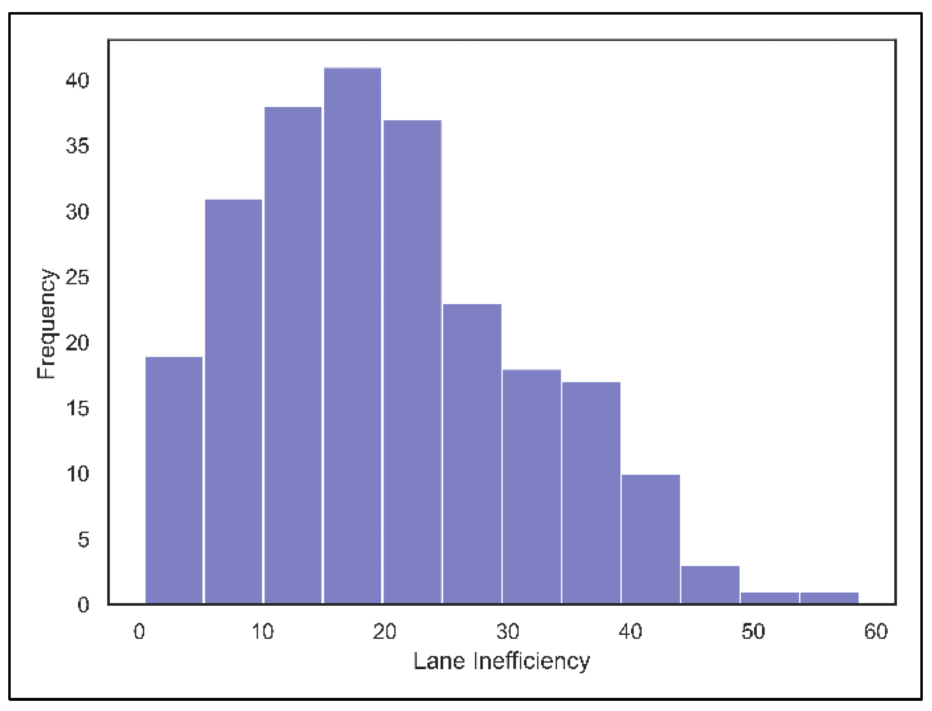
5.1. Descriptive Evaluation of the Lane Inefficiency Values

Throughout the field study, a total of 586 green periods were observed from video recordings. As mentioned earlier, green periods with fewer than eight vehicles in the queue, as well as green periods in which the time headway of the first vehicle was less than 2 s, were excluded (see

Table 3. Number of studied green periods.

Intersection	Approach	Observed	Q < 8	h1 < 2	Efficient	Studied
Mall	West	142	23	13	13	93
	East	142	94	8	2	38
	North	145	93	0	0	52
Expo	West	157	74	23	4	56
Total		586	284	44	19	239

). The results indicated that some cycles were efficient (i.e., $\sum {\mu }_i>{\lambda }_i$). These green periods were also excluded from the analysis.

Table 4. Properties of the inefficient green periods.

Intersection		Mall			Expo
Approach		West	East	North	West
Number of green periods		93	38	52	56
Green time (s)	Min.	31	19	20	18
	Avg.	56	32	25	23
	Max.	72	35	30	33
Red time (s)	Min.	30	42	58	63
	Avg.	46	66	78	69
	Max.	78	77	90	91
Queue length (veh/lane)	Min.	8	8	8	8
	Avg.	14.0	11.0	10.0	10.6
	Max.	25	15	15	15
Traffic composition (%)	PC	94.3	92.2	97.3	92.5
	PT	4.6	2.4	2.7	5.1
	HV	1.1	5.4	0.0	2.4

presents the properties of the studied green periods. The distribution of lane inefficiency values for these green periods is shown in Figure 5 (239 green periods). The lane inefficiency values ranged from 0.40% to 58.60%. The median lane inefficiency was determined to be 19%, with a mean of %11.60.

5.2. Statistical Modeling Results

5.2.1. Principal Component Analysis (PCA) Results

PCA is a technique employed for the analysis of large datasets, aiding in the visualization of multidimensional data in order to enhance data interpretability [52,53]. Additionally, PCA is utilized for the detection, quantification, and resolution of multicollinearity in a dataset [54].

PCA was conducted on the entire dataset, incorporating all nine independent variables with orthogonal rotation using varimax. The Kaiser–Meyer–Olkin (KMO) measure, assessing the sampling adequacy for the analysis, yielded a value of 0.583, surpassing the recommended threshold of 0.50, as suggested by Kaiser [55]. Additionally, Bartlett’s test of sphericity, resulting in χ² (586) = 2560.408, with p < 0.001, indicated that the outcomes of the PCA analysis achieved statistical significance. The outcomes of the PCA analysis are shown in

Table 5. The results of the PCA analysis.

Total Variance Explained
Component	Initial Eigenvalues			Extraction Sums of Squared Loadings			Rotation Sums of Squared Loadings
	Total	% of Variance	Cum. %	Total	% of Variance	Cum. %	Total	% of Variance	Cum. %
1	3.711	41.230	41.230	3.711	41.230	41.230	3.643	40.479	40.479
2	2.245	24.948	66.178	2.245	24.948	66.178	1.924	21.375	61.853
3	1.286	14.292	80.469	1.286	14.292	80.469	1.675	18.616	80.469
4	0.804	8.933	89.402
5	0.571	6.340	95.743
6	0.285	3.171	98.913
7	0.060	0.668	99.581
8	0.031	0.343	99.924
9	0.007	0.076	100.000

. The output revealed three components with eigenvalues exceeding the threshold of “1,” collectively explaining 80.469% of the variance. The PCA analysis results proposed three distinct components, as outlined in

Table 6. Rotated component matrix.

Variable	Component
	1	2	3
G	0.971
g/C	0.943
θ		0.913
θ/G		0.933
Q	0.801
V	0.982
VHV			0.650
ϕ			0.636
β			−0.837

. The variables in the first component (G, g/C, Q, and V) explained 40.479% of the variance, followed by the second component (θ and θ/G), which explained 21.375%. Finally, the last component (V, ϕ, and β), the total time headway of the first four vehicles in the queue and average discharge rate, explained 18.616% of the variance.

In light of these findings, it is imperative to incorporate variables from all three components during the development of multiple linear regression models. It is advised to refrain from employing various variables obtained from a single component, given their pronounced levels of correlation. This approach is essential to ensuring the robustness and diversity of the selected variables in the regression models [56].

5.2.2. Multiple Linear Regression Analysis Results

Linear regression analysis relies on the assumption that the independent variables used in a model are statistically uncorrelated with each other. Therefore, it is crucial to confirm whether these variables meet this assumption through a Pearson correlation analysis. Figure 6 depicts the correlation coefficients among the independent variables. Correlation coefficients with an absolute value exceeding 0.60 or 0.70 indicate a strong correlation between variables [57].

The Pearson correlation analysis yielded similar results to the PCA analysis:

• Green time (G), the ratio of the effective green time to the cycle time (g/C), queue length (Q), and departure volume (V) are highly correlated with each other (variables in component 1);
• The ratio of total unused green time to green time (θ/G) is highly positively correlated with total unused green time (θ) (variables in component 2).

As a result, in the developed models, the use of more than one variable from both component 1 and component 2 was avoided to mitigate potential multicollinearity issues. Various models have been developed to illustrate the impact of different independent variables on lane inefficiency. The results of the most significant models are presented in

Table 7. Results of the multiple linear regression analysis.

Model	Independent Variables	Coeff.	p-Value	R2
1	Green time (G)	0.170	0.000	0.730
	Total unused green time/green time (θ/G)	116.662	0.000
2	Green time (G)	0.179	0.000	0.618
	Total unused green time (θ)	2.336	0.000
	Percentage of heavy vehicles in departure volume (VHV)	0.620	0.005
3	Total unused green time (θ)	1.321	0.000	0.835
	Effective green time/cycle time (g/C)	−37.855	0.000
	Total time headways of the first four vehicles (ϕ)	2.655	0.000
4	Total unused green time/green time (θ/G)	42.464	0.000	0.844
	Queue length (Q)	−1.020	0.000
	Total time headways of the first four vehicles (ϕ)	2.546	0.000

. The adjusted R-squared values for all the different models are high, ranging from 0.618 to 0.844.

The subsequent findings are outlined below:

• Model 1: The combination of green time (G) and the ratio of total unused green time to green time (θ/G) accounted for 73%, a significant proportion, of the total variability in lane inefficiency. Of particular note is the substantial influence of the latter variable on lane inefficiency, as indicated by its standardized coefficient (Coefficient = 116.662, p-value = 0.000).
• Model 2: Green time (G), total unused green time (θ), and the percentage of heavy vehicles (VHV) were identified as significant factors contributing positively to lane inefficiency. This model attained an adjusted R-squared value of 0.618.
• Model 3: Demonstrating higher predictive power with an R-squared value of 0.835, this model revealed positive associations between total unused green time (θ), the total time headways of the first four vehicles (ϕ), and lane inefficiency. Conversely, the ratio of effective green time to cycle time (g/C) exhibited a negative association with lane inefficiency (Coefficient = −37.855, p-value < 0.000).
• Model 4: This model yielded the highest adjusted R-squared value. It suggested that (a) an increase in the ratio of total unused green time to green time (θ/G) and total time headways of the first four vehicles (ϕ) increases lane inefficiency. On the other hand, an increase in queue length (Q) decreases lane inefficiency.

6. Conclusions and Discussion

This study focused on understanding the efficiency of vehicle discharge at the saturation flow rate during the green period at intersections controlled by fully actuated signal systems. The saturation flow rate, representing maximum vehicle discharge under optimal conditions, plays a crucial role in intersection capacity and traffic signal system planning. It is a key parameter explored in this research, holding significance not only for intersection capacity but also for the overarching goal of sustainable traffic management. Efficient signal systems contribute directly to reducing traffic congestion, subsequently decreasing emissions and enhancing overall air quality in urban areas. This connection underscores this study’s relevance to the broader context of environmental sustainability.

This study introduced a novel parameter, lane inefficiency, to assess vehicle discharge efficiency during green period. Calculated by comparing the saturation flow rate with the instant discharge rate, this parameter offers a comprehensive evaluation of green period utilization for a specific lane. In this research, we investigated signal control system parameters (e.g., green time, red time, and cycle time) and traffic flow parameters (e.g., queue length, departure flow, and vehicle composition) using PCA and multiple linear regression models, contributing to a holistic understanding of factors influencing the green period’s efficient use. Additionally, sustainability in urban transportation can be promoted through the practical insights provided by this study on fully actuated signal systems. When applied, the following findings contribute directly to creating smarter, more efficient, and environmentally conscious urban mobility systems:

• The variables of green time (G), the ratio of total unused green time to green time (θ/G), the total unused green time (θ), the percentage of heavy vehicles in the departure volume (VHV), the ratio of effective green time to cycle time (g/C), the total time headways of the first four vehicles (ϕ), and queue length (Q) were identified as significant factors.
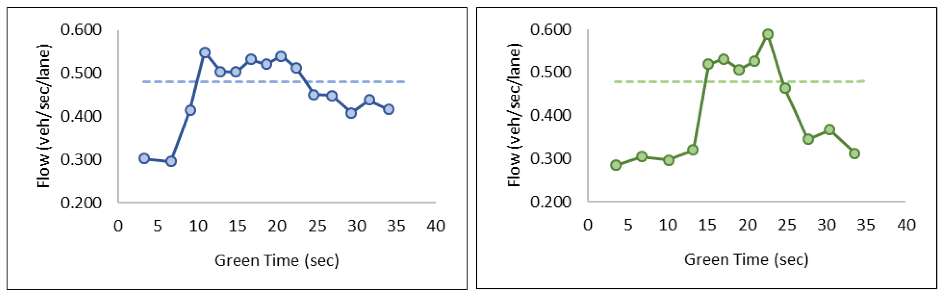
• Extended green times (G) contribute to increased lane inefficiency (δ). This phenomenon results from a decreased discharge rate in the later part of the green period. Therefore, the time headways surpass the saturated time headways at the end of green periods.
• The total unused green time (θ) at the start of the green period as well as the ratio of total unused green time to green time (θ/G) both contribute to a rise in lane inefficiency (δ). This indicates that delays induced by the initial vehicles crossing the stop line negatively affect traffic flow. In contrast, there was an observed decrease in lane inefficiency (δ) with an increase in the ratio of effective green time to cycle time (g/C). This observation underscores the adverse impact of time losses on traffic flow.
• The results highlight a notable correlation between the percentage of heavy vehicles (VHV) and the escalation of lane inefficiency (δ). This phenomenon can be elucidated by considering the cautious driving behavior of passenger car drivers when sharing the road with heavy vehicles. The heightened presence of heavy vehicles appears to instigate a decrease in the discharge flow rate, contributing to the observed increase in lane inefficiency (δ).
• It was observed that lane inefficiency (δ) experiences an increase as queue length (Q) decreases. This phenomenon can be attributed to a shorter queue length, where a substantial portion of the green period is often occupied by non-queue vehicles characterized by greater time headways. In contrast, as the queue length increases, a larger portion of the green period tends to be occupied by queue vehicles with smaller time headways, resulting in a decrease in lane inefficiency. This highlights the relationship between queue length dynamics and their influence on the efficiency of traffic flow during green periods.
• This investigation reveals a noteworthy trend wherein lane inefficiency (δ) tends to rise with an increase in the total time headway of the first four vehicles in a queue (ϕ). The total time headway of the first four vehicles in the queue (ϕ) signifies the total time needed to attain saturation conditions. When the traffic flow reaches saturation flow later, denoting a higher ϕ value, the inherent consequence is an increase in lane inefficiency (δ).

The findings pointed out insights into aspects like green times, the influence of heavy vehicles, and the queue length, suggesting ideas for specific actions that can improve traffic signal timing and minimize environmental impacts. This directly supports the sustainable utilization of urban infrastructure. This study emphasizes the dynamic interaction between different factors and lane inefficiency, giving practical insights for urban planners and policymakers. Adjusting various parameters related to traffic improves overall traffic flow efficiency, decreases fuel consumption, and reduces emissions, aligning with broader sustainability objectives for efficient and environmentally friendly transportation. In summary, this research delves into fully actuated signal systems, enhancing our understanding of traffic dynamics and proposing practical measures to encourage sustainability in urban transportation. Consequently, it contributes to the creation of more intelligent, efficient, and environmentally friendly urban mobility systems.

7. Limitations and Further Recommendations

While this study offers valuable insights, a primary limitation arises from its exclusive focus on the middle lanes of approach legs at intersections. Enhancing the proposed method so that it includes other lanes and accounts for factors such as right-/left-turning vehicles and lane-changing behaviors could amplify the generalizability of the findings, which could be achieved in further studies. This suggests a promising avenue for future research with the aim of delving into a more comprehensive understanding of traffic dynamics. However, it is crucial to emphasize that the proposed methodology remains readily applicable and easily adoptable for assessing lane efficiency in various intersection scenarios.

References

1. Cipriani, E.; Mannini, L.; Montemarani, B.; Nigro, M.; Petrelli, M. Congestion pricing policies: Design and assessment for the city of Rome, Italy. Transp. Policy 2019, 80, 127–135. [Google Scholar] [CrossRef]
2. Mondal, S.; Gupta, A. A review of methodological approaches for saturation flow estimation at signalized intersections. Can. J. Civ. Eng. 2020, 47, 237–247. [Google Scholar] [CrossRef]
3. Wong, S.C.; Sze, N.N.; Li, Y.C. Contributory factors to traffic crashes at signalized intersections in Hong Kong. Accid. Anal. Prev. 2007, 39, 1107–1113. [Google Scholar] [CrossRef] [PubMed]
4. Wang, J.; Guo, X.; Yang, X. Efficient and safe strategies for intersection management: A review. Sensors 2021, 21, 3096. [Google Scholar] [CrossRef] [PubMed]
5. Gong, Y.J.; Zhang, J. Real-time traffic signal control for modern roundabouts by using particle swarm optimization-based fuzzy controller. arXiv 2014, arXiv:1408.0689. [Google Scholar]
6. Cai, C.; Wong, C.K.; Heydecker, B.G. Adaptive traffic signal control using approximate dynamic programming. Transp. Res. Part C Emerg. Technol. 2009, 17, 456–474. [Google Scholar] [CrossRef]
7. Ali, M.E.M.; Durdu, A.; Çeltek, S.A.; Yilmaz, A. An adaptive method for traffic signal control based on fuzzy logic with webster and modified webster formula using SUMO traffic simulator. IEEE Access 2021, 9, 102985–102997. [Google Scholar] [CrossRef]
8. Fan, J.; Najafi, A.; Sarang, J.; Li, T. Analyzing and Optimizing the Emission Impact of Intersection Signal Control in Mixed Traffic. Sustainability 2023, 15, 16118. [Google Scholar] [CrossRef]
9. Majstorović, Ž.; Tišljarić, L.; Ivanjko, E.; Carić, T. Urban Traffic Signal Control under Mixed Traffic Flows: Literature Review. Appl. Sci. 2023, 13, 4484. [Google Scholar] [CrossRef]
10. Du, Y.; Kouvelas, A.; ShangGuan, W.; Makridis, M.A. Dynamic capacity estimation of mixed traffic flows with application in adaptive traffic signal control. Phys. A Stat. Mech. Its Appl. 2022, 606, 128065. [Google Scholar] [CrossRef]
11. Zheng, X.; Recker, W.; Chu, L. Optimization of control parameters for adaptive traffic-actuated signal control. J. Intell. Transp. Syst. 2010, 14, 95–108. [Google Scholar] [CrossRef]
12. Morozov, V.; Shepelev, V.; Kostyrchenko, V. Modeling the operation of signal-controlled intersections with different lane occupancy. Mathematics 2022, 10, 4829. [Google Scholar] [CrossRef]
13. Leitner, D.; Meleby, P.; Miao, L. Recent advances in traffic signal performance evaluation. J. Traffic Transp. Eng. 2022, 9, 507–531. [Google Scholar] [CrossRef]
14. Lattimer, C.R. Automated Traffic Signals Performance Measures. FWHA-HOP-20-002; Federal Highway Administration: Washington, DC, USA, 2020.
15. Gettman, D.; Folk, E.; Curtis, E.; Ormand, K.K.D.; Mayer, M.; Flanigan, E. Measures of Effectiveness and Validation Guidance for Adaptive Signal Control Technologies; Federal Highway Administration: Washington, DC, USA, 2013.
16. Fourati, W.; Friedrich, B. Trajectory-based measurement of signalized intersection capacity. Transp. Res. Rec. 2019, 2673, 370–380. [Google Scholar] [CrossRef]
17. Maxwell, A.; Wood, K. Review of traffic signals on high-speed roads. In Proceedings of the European Transport Conference (ETC) Association for European Transport (AET), Strasbourg, France, 18–20 September 2006. [Google Scholar]
18. He, F.; Yan, X.; Liu, Y.; Ma, L. A traffic congestion assessment method for urban road networks based on speed performance index. Procedia Eng. 2016, 137, 425–433. [Google Scholar] [CrossRef]
19. Taylor, R. Travel Time Reliability: Making It There on Time, All the Time. FHWA-HOP-06-070; Federal Highway Administration: Washington, DC, USA, 2006.
20. Margiotta, R.A.; Turner, S.; Taylor, R.; Chang, C. National Performance Measures for Congestion, Reliability, and Freight, and CMAQ Traffic Congestion: General Guidance and Step-by-Step Metric Calculation Procedures (No. FHWA-HIF-18-040). 2018. Available online: https://trid.trb.org/view/1528656 (accessed on 14 July 2023).
21. Chen, P.; Sun, J.; Qi, H. Estimation of delay variability at signalized intersections for urban arterial performance evaluation. J. Intell. Transp. Syst. 2017, 21, 94–110. [Google Scholar] [CrossRef]
22. Transportation Research Board (TRB). Highway Capacity Manual, 5th ed.; Transportation Research Board, National Research Council: Washington, DC, USA, 2010. [Google Scholar]
23. Saha, P.; Roy, R.; Sarkar, A.K.; Pal, M. Preferred time headway of drivers on two-lane highways with heterogeneous traffic. Transp. Lett. 2019, 11, 200–207. [Google Scholar] [CrossRef]
24. Wu, S.; Zou, Y.; Wu, L.; Zhang, Y. Application of Bayesian model averaging for modeling time headway distribution. Phys. A Stat. Mech. Its Appl. 2023, 620, 128747. [Google Scholar] [CrossRef]
25. Knoop, V.; Hoogendoorn, S. Free Flow Capacity and Queue Discharge Rate: Long-Term Changes. Transp. Res. Rec. 2022, 2676, 483–494. [Google Scholar] [CrossRef]
26. Li, H.; Prevedouros, P.D. Detailed observations of saturation headways and start-up lost times. Transp. Res. Rec. 2002, 1802, 44–53. [Google Scholar] [CrossRef]
27. Denney, R.W., Jr.; Curtis, E.; Head, L. Long green times and cycles at congested traffic signals. Transp. Res. Rec. 2009, 2128, 1–10. [Google Scholar] [CrossRef]
28. Khosla, K.; Williams, J.C. Saturation flow at signalized intersections during longer green time. Transp. Res. Rec. 2006, 1978, 61–67. [Google Scholar] [CrossRef]
29. Lin, F.B.; Thomas, D.R. Headway compression during queue discharge at signalized intersections. Transp. Res. Rec. 2005, 1920, 81–85. [Google Scholar] [CrossRef]
30. Gao, L.; Alam, B. Optimal discharge speed and queue discharge headway at signalized intersections. In Proceedings of the 93rd Annual Meeting of Transportation Research Board, Washington, DC, USA, 12–16 January 2014. [Google Scholar]
31. Liu, X.; Yu, J.; Yang, X. Diagnostic-oriented and evaluation-driven framework for bus route performance improvement. J. Transp. Eng. Part A Syst. 2021, 147, 04021030. [Google Scholar] [CrossRef]
32. Chen, P.; Nakamura, H.; Asano, M. Saturation flow rate analysis for shared left-turn lane at signalized intersections in Japan. Procedia-Soc. Behav. Sci. 2011, 16, 548–559. [Google Scholar] [CrossRef]
33. Shao, C.Q.; Rong, J.; Liu, X.M. Study on the saturation flow rate and its influence factors at signalized intersections in China. Procedia-Soc. Behav. Sci. 2011, 16, 504–514. [Google Scholar] [CrossRef]
34. Potts, I.B.; Ringert, J.F.; Bauer, K.M.; Zegeer, J.D.; Harwood, D.W.; Gilmore, D.K. Relationship of lane width to saturation flow rate on urban and suburban signalized intersection approaches. Transp. Res. Rec. 2007, 2027, 45–51. [Google Scholar] [CrossRef]
35. Qin, Z.; Zhao, J.; Liang, S.; Yao, J. Impact of guideline markings on saturation flow rate at signalized intersections. J. Adv. Transp. 2019, 2019, 1–13. [Google Scholar]
36. Davoodi, S.R.; Sadeghiyan, S.; Faezi, S.F. The Analysis the Role of Motorcycles on Saturation Flow Rates at Signalized Intersections in Gorgan. Indian J. Sci. Technol. 2015, 8, 1–6. [Google Scholar] [CrossRef]
37. Chen, P.; Qi, H.; Sun, J. Investigation of saturation flow on shared right-turn lane at signalized intersections. Transp. Res. Rec. 2014, 2461, 66–75. [Google Scholar] [CrossRef]
38. Wang, Y.; Rong, J.; Zhou, C.; Chang, X.; Liu, S. An analysis of the interactions between adjustment factors of saturation flow rates at signalized intersections. Sustainability 2020, 12, 665. [Google Scholar] [CrossRef]
39. Mondal, S.; Arya, V.K.; Gupta, A.; Gunarta, S. Comparative analysis of saturation flow using various PCU estimation methods. Transportation Research Procedia 2020, 48, 3153–3162. [Google Scholar] [CrossRef]
40. Lu, Z.; Kwon, T.J.; Fu, L. Effects of winter weather on traffic operations and optimization of signalized intersections. J. Traffic Transp. Eng. 2019, 6, 196–208. [Google Scholar] [CrossRef]
41. Devalla, J.; Biswas, S.; Ghosh, I. The effect of countdown timer on the approach speed at signalised intersections. Procedia Comput. Sci. 2015, 52, 920–925. [Google Scholar] [CrossRef]
42. Zhao, J.; Yu, J.; Zhou, X. Saturation flow models of exit lanes for left-turn intersections. J. Transp. Eng. Part A Syst. 2019, 145, 04018090. [Google Scholar] [CrossRef]
43. Gao, X.; Zhao, J.; Wang, M. Modelling the saturation flow rate for continuous flow intersections based on field collected data. PLoS ONE 2020, 15, e0236922. [Google Scholar] [CrossRef] [PubMed]
44. Wang, Y.; Rong, J.; Zhou, C.; Gao, Y. Dynamic estimation of saturation flow rate at information-rich signalized intersections. Information 2020, 11, 178. [Google Scholar] [CrossRef]
45. Mondal, S.; Gupta, A. Non-linear evaluation model to analyze saturation flow under weak-lane-disciplined mixed traffic stream. Transp. Res. Rec. 2021, 2675, 422–431. [Google Scholar] [CrossRef]
46. Patel, P.N.; Dhamaniya, A. Developing mixed traffic equivalency factors to estimate saturation flow at urban signalized intersections. Transp. Res. Rec. 2021, 2675, 601–611. [Google Scholar] [CrossRef]
47. Dehman, A.; Farooq, B. Capacity characteristics of long-term work zones on signalized intersection approaches. Transp. Res. Part A Policy Pract. 2023, 175, 103791. [Google Scholar] [CrossRef]
48. Liu, X.; Lai, L.; Kong, Y.; Le Vine, S. Protected turning movements of noncooperative automated vehicles: Geometrics, trajectories, and saturation flow. J. Adv. Transp. 2018, 2018, 1–12. [Google Scholar] [CrossRef]
49. Song, L.; Fan, W. Intersection capacity adjustments considering different market penetration rates of connected and automated vehicles. Transp. Plan. Technol. 2023, 46, 286–303. [Google Scholar] [CrossRef]
50. Day, C.M.; Sturdevant, J.R.; Li, H.; Stevens, A.; Hainen, A.M.; Remias, S.M.; Bullock, D.M. Revisiting the cycle length: Lost time question with critical lane analysis. Transp. Res. Rec. 2013, 2355, 1–9. [Google Scholar] [CrossRef]
51. Ross, S.M. Introduction to Probability and Statistics for Engineers and Scientists; Academic Press: Cambridge, MA, USA, 2014. [Google Scholar]
52. Hastie, T.; Tibshirani, R.; Friedman, J.H.; Friedman, J.H. The Elements of Statistical Learning: Data Mining, Inference, and Prediction; Springer: New York, NY, USA, 2009; Volume 2, pp. 1–758. [Google Scholar]
53. Beattie, J.R.; Esmonde-White, F.W. Exploration of principal component analysis: Deriving principal component analysis visually using spectra. Appl. Spectrosc. 2021, 75, 361–375. [Google Scholar] [CrossRef]
54. Lafi, S.Q.; Kaneene, J.B. An explanation of the use of principal-components analysis to detect and correct for multicollinearity. Prev. Vet. Med. 1992, 13, 261–275. [Google Scholar] [CrossRef]
55. Kaiser, H.F. An index of factorial simplicity. Psychometrika 1974, 39, 31–36. [Google Scholar] [CrossRef]
56. Cevher, O.; Altintasi, O.; Tuydes-Yaman, H. Evaluating the relation between station area design parameters and transit usage for urban rail systems in Ankara, Turkey. Int. J. Civ. Eng. 2020, 18, 951–966. [Google Scholar] [CrossRef]
57. Hosseinzadeh, A.; Algomaiah, M.; Kluger, R.; Li, Z. Spatial analysis of shared e-scooter trips. J. Transp. Geogr. 2021, 92, 103016. [Google Scholar] [CrossRef]
Figure 1. Locations of the studied intersections.
Sustainability 16 00722 g001
Figure 2. The concept of lane inefficiency.
Sustainability 16 00722 g002
Figure 3. Flowchart of the proposed methodology.
Sustainability 16 00722 g003
Figure 4. Saturation flow rate and instant discharge rate.
Sustainability 16 00722 g004
Figure 5. Distribution of the lane inefficiency values.
Sustainability 16 00722 g005
Figure 6. Correlation matrix of the independent variables.
Sustainability 16 00722 g006