Analyzing Technical Efficiency in Cereal Production across Selected European Union Countries

Abstract

This paper investigates the technical efficiency of cereal production in European Union (EU) countries from 2008 to 2018. The primary purpose is to estimate technical efficiency scores by country and crop and explain their variation using macroeconomic and agricultural policy variables using the stochastic frontier production function. The results indicate that the United Kingdom has the highest efficiency in barley production, while Finland has the lowest. France exhibits the highest efficiency in common wheat, and Romania has the lowest efficiency in grain maize production. This study also explores the impact of various factors on technical efficiency, finding, for example, the positive effects of female wages and foreign direct investment on barley production efficiency and the negative effects of forest area and subsidies. Similar analyses were conducted for wheat and maize production. The results indicate a variation in technical efficiency scores across crops and countries. This diversity in performance not only reflects the inherent complexities within each crop but also emphasizes the crucial role played by macroeconomic variables and agricultural policies in shaping efficiency outcomes on a country-wide scale.

1. Introduction

Despite the technological advances in the past century, agriculture remains critical in advancing and preserving human welfare. In addition, the future of humanity depends on the stability and sustainability of agricultural production. However, the land available to allocate to agriculture is limited, and with more urbanization, it may even shrink. Because of this, agriculture is one of the most critical areas that policy-makers in Europe are focusing on due to agriculture’s significant contribution to the European economy. They argue that improving agricultural productivity is crucial for raising farmer income and the survival of humanity [1,2]

According to Schils et al. [3], European countries are among the highest cereal producers globally, producing 20% of total global production and exporting 15% of that production. Schils et al. [3] also mentioned that approximately one-fourth of that production is for human consumption. Furthermore, Europe’s crop production accounts for a third of the total agricultural land and approximately 60% of the total crops, with barley, sorghum, and oats used for livestock feed. In contrast, wheat is used nearly equally for human use. However, agriculture is highly dependent on land conditions, seasonal terms, and the climate. The economies of several European Union countries are strongly reliant on agriculture, and crop production is one of the most common livelihood sources in rural Europe. Despite being developed countries, Europe’s overall gross value added to agriculture has grown by 1.7% per year. The changes in national agricultural institutions, the effects of globalization, and many other variables, such as the agricultural policy that the European countries have established, have played the most significant role in this regard [4].

Revisions to agricultural policies were made throughout the 1990s as new concerns emerged and further information was obtained. Driven by changes in the global economy and the sector, European countries are enacting new legislation to increase agricultural efficiency. The government requires the private sector and producers to adhere to specific standards [5]. In this regard, European governments designed the common agricultural policy (CAP) to promote complementary sectors and producers via various programs encouraging farmers to adopt sustainable and efficient farming practices. Moreover, the European Union implements standards in farming (such as quality and environmental protection) and produces more outputs while using fewer inputs. As evidenced by these recent advances, many scholars believe that sustainable agricultural and natural resource usage are critical to many nations’ policies, particularly those of the European Union.

Since the implementation of the new rules, which also affect the private sector and agricultural industry operations, agricultural efficiency has been at the center of many debates in agricultural production. Adopting more efficient agricultural practices for the private sector is helpful as it reduces costs. It also reduces the detrimental environmental impacts, enhances food security, and contributes to the attainment of sustainable development goals, with food security as a central focus. For all these reasons, measuring efficiency is as critical to these objectives as attaining it. To elaborate, improving efficiency is essential because it allows farmers to produce more output without using more inputs, thus reducing costs or at least preventing an increase in the cost of production. Consequently, it is unsurprising that much work has been dedicated to investigating farm-level efficiency in developed and developing countries. However, if farmers are not optimally using present technology to boost efficiency, enhancing efficiency is a more economically efficient strategy than implementing new technologies.

Introducing the most efficient production technologies is one of the most effective strategies to guarantee that producers can produce in the best and most lucrative manner. Efficiency is essential due to a lack of natural endowments and financial constraints. Moreover, the efficiency evaluation is vital since it is considered the most suitable way for these producers to evaluate how much productivity can be enhanced by optimizing the number of resources used while at the same time boosting their production and profit. Additionally, efficiency determines whether growing productivity or developing new technologies should be the company’s primary emphasis to be the leading company in different aspects of agricultural production [6]. In this regard, the mismanagement of resource allocation is also emphasized since it affects productivity.

Assessing technical efficiency in developed and developing nations is still an essential field of study [6]. Particularly relevant for the agriculture sector, when resources are limited and subject to environmental and government regulations, greater production is driven by improved technical efficiency. Hence, the estimation of efficiency is essential because it is the most significant measure for productivity growth and reduction in inefficiency. For the farmers, being aware of the efficiency levels of their production will help them allocate resources more effectively, reduce the loss of soil quality, reduce the cost, and eventually increase profit.

Therefore, the primary purpose of this study is to estimate the level of technical efficiency for cereal products (barley, common wheat, and grain maize) across some European countries. In addition, this study uses macroeconomic variables like GDP, unemployment rate, and inflation and agricultural policy variables such as total direct subsidies, decoupled subsidies, and livestock subsidies to explain the variation of the technical efficiency scores across crops and European countries. One of the novelties of this study is that we estimate technical efficiency at the country level rather than just at the firm level, providing a comprehensive understanding of the overall efficiency landscape within a country’s cereal production sector. This approach considers macroeconomic variables and agricultural policies, identifying trends, patterns, and disparities in technical efficiency across countries. It also allows for targeted policy recommendations and interventions at the national level, leading to sustainable improvements in cereal production practices. The other novelty of this study is that we use machine learning techniques, specifically random forest regression, to help us identify the most important inputs to be used as independent variables for each crop in the estimation of the production function. This study also uses the random forest technique to determine the economic and policy variables that enter the inefficiency component of the production function. The random forest technique allows only the most influential explanatory variables, saving the degrees of freedom due to the small sample size.

Furthermore, we assess the degree of technical efficiency and its variability across various crops and countries by employing stochastic frontier analysis, incorporating a random effect model under three distinct distributional assumptions (half-normal, exponential, and truncated-normal). Furthermore, we also estimate the impact of macroeconomic and agricultural policy variables on the overall level of technical efficiency across crops and countries. Finally, using Vuong’s test [7], we compare the stochastic frontier model (a random effect model) implied by the three distributions and determine which model best fits the sample data.

Efficiency variations are caused by changes in the size of the operation, manufacturing technology, operating conditions, and operational efficiency [8]. According to [9], efficiency helps farmers increase their output without increasing or changing the number of inputs used in the production process. The concept of efficiency also arises to avoid wasting overexploited resources such as land, water, energy, and fertilizers. In doing so, this assists farmers in efficiently allocating scarce inputs to be suitable for producing higher output. Therefore, efficiency measurement is critical since farmers need to improve agricultural production while utilizing limited resources.

Furthermore, because resources such as land, energy, water, and fertilizers are essential in agricultural production, producers must use them efficiently to avoid overconsumption, which wastes resources and may deplete soil quality and exacerbate scarcity of water and food insecurity. For this reason, governments often put regulations and restrictions on farmers to make them use resources efficiently in a suitable way for continuing population growth, adaptation to climate change, consumption growth, and reduction in the overexploitation of the environment. At the same time, from an economic standpoint, governments may employ subsidies to achieve a more efficient allocation of resources by incentivizing farmers to change production decisions or adopt more efficient production technologies [10].

One such policy was the Common Agricultural Policy (CAP) (a collaborative and shared policy embraced by all European Union nations, with the goal of assisting farmers in enhancing productivity, which established a pact between agriculture and society, as well as between Europe and its producers) instituted in 1962 by the European Union. One of the goals of the Common Agricultural Policy (CAP) is to assist farmers, enhance agricultural productivity, ensure a consistent supply of affordable food, and contribute to addressing climate change while promoting the sustainable management of natural resources (European Commission, n.a.). One of the primary vehicles the CAP uses to achieve its objectives is providing income support or subsidies through direct payments, decoupled payments, livestock payments, and remunerating farmers for practicing environmentally friendly farming.

Several studies have been undertaken to evaluate the efficiency and its determinants among various kinds of farmers and regions (see, for example, [2,6,11,12,13,14,15,16,17,18,19,20,21]). These studies aimed to explain the technical efficiency of diverse crops and farms in the same country concerning the same inputs in general or by varying the specific inputs for each farm or crop. Furthermore, many studies also examine the sources of the technical efficiency for crops or farms to identify the variables, such as family labor, level of education, contract work, farm size, and farmer age, that affect the efficiency of farms or crops. As such, crop efficiency studies help educate us about farmer productivity and performance regarding the inputs.

At the same time, these studies have established that various factors cause differences in farmers’ production efficiency. As a result, it makes sense not to limit these studies to an analysis of only the inputs but also to include macroeconomic variables such as GDP and inflation. In the context of Europe (see, e.g., [11,22,23]), while many studies have looked into understanding the technical inefficiency determinants in crop production, none of these studies have considered studying the efficiency levels for the same crops across countries and how efficiency is sensitive to macroeconomic variables and subsidies. Therefore, this study estimates technical efficiency for various crops, including common wheat, grain maize, and barley. It determines the level of technical efficiency using data from Europe’s Farm Accountancy Data Network (FADN) and the World Bank. We estimate technical efficiency using stochastic frontier analysis (SFA), and its variation is explained by macroeconomic and agricultural policy variables (subsidies) across different countries. In other words, we evaluate how macroeconomic factors such as GDP, inflation, and unemployment rate and policy variables, such as subsidies originating from the Common Agricultural Policy (CAP), contribute to the sources of technical inefficiency. We use machine learning techniques, specifically random forest regression, to extract the most important inputs to be used as independent variables for each crop in the production function estimation. This study also uses the random forest technique to determine the economic and policy variables that enter the inefficiency component of the production function.

The rest of the paper is organized as follows. First, in Section 2, we describe the conceptual framework. Then, Section 3 describes the data and the empirical estimation. Finally, in Section 4, we present and discuss the results; in Section 5, we conclude and suggest future research avenues.

2. Conceptual Framework

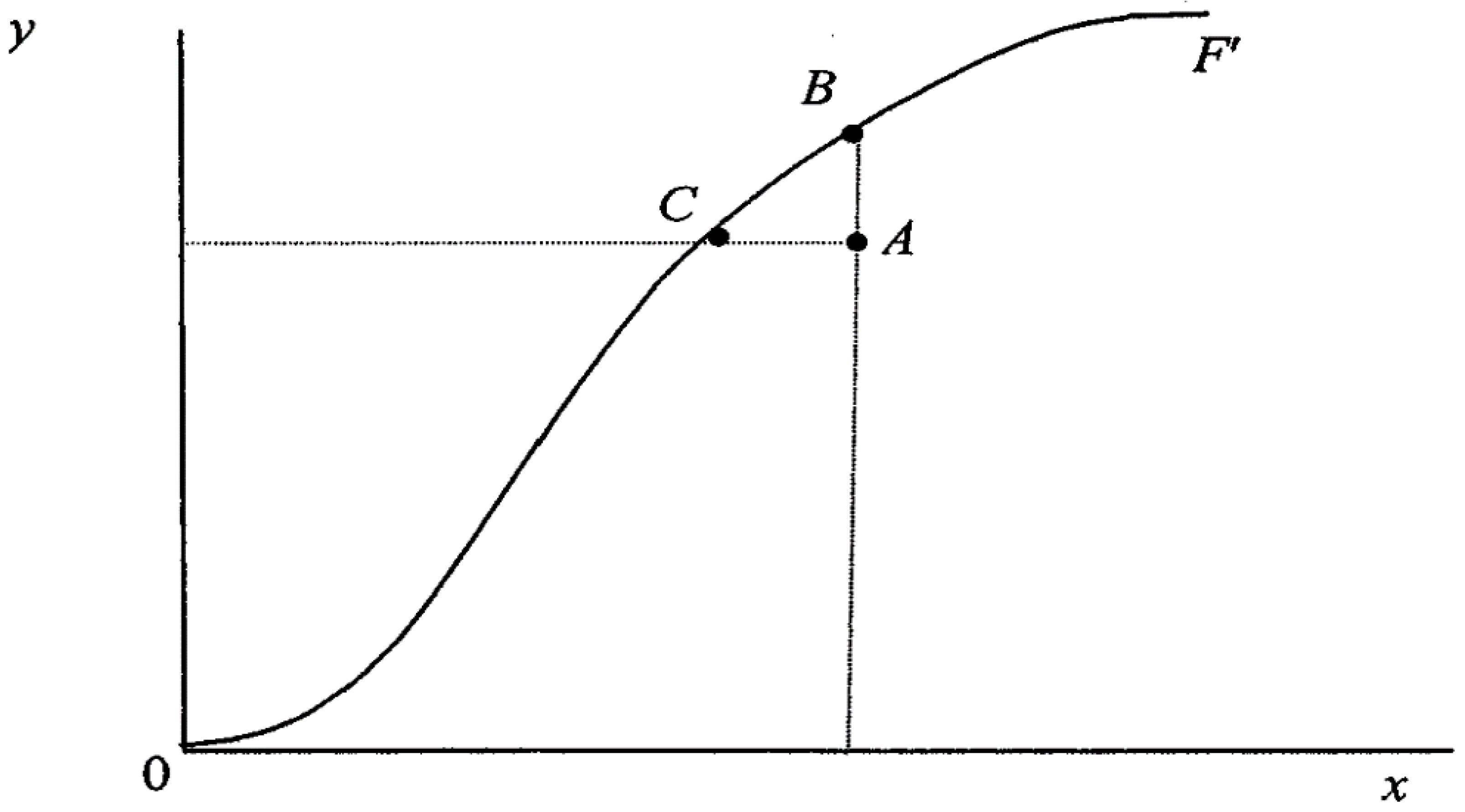
Coelli et al. [24] identified a production frontier curve that describes the connection between inputs and output. Thus, the production frontier denotes the maximum output obtained from the combination of inputs used in the production process. Graphically, the production frontier curve can be represented in Figure 1 with the inputs, x, on the horizontal axis, and the output level, y, on the vertical axis. Firms in the industry operate either on the frontier if they are technically efficient or below the frontier curve if they are not efficient for various reasons.

For instance, consider point A as an inefficient position, while points B and C represent efficient locations. Therefore, a company operating at point A is deemed inefficient since it has the potential to increase production to the level associated with either point B without requiring additional inputs for higher output or using fewer inputs to produce the same output as in point C. The diagram also conveys the concept of a feasible production set, encompassing all conceivable input–output combinations between the production line $OF$ and the x axis. The subset of this viable production set that represents efficiency is characterized by points along the production frontier [24].

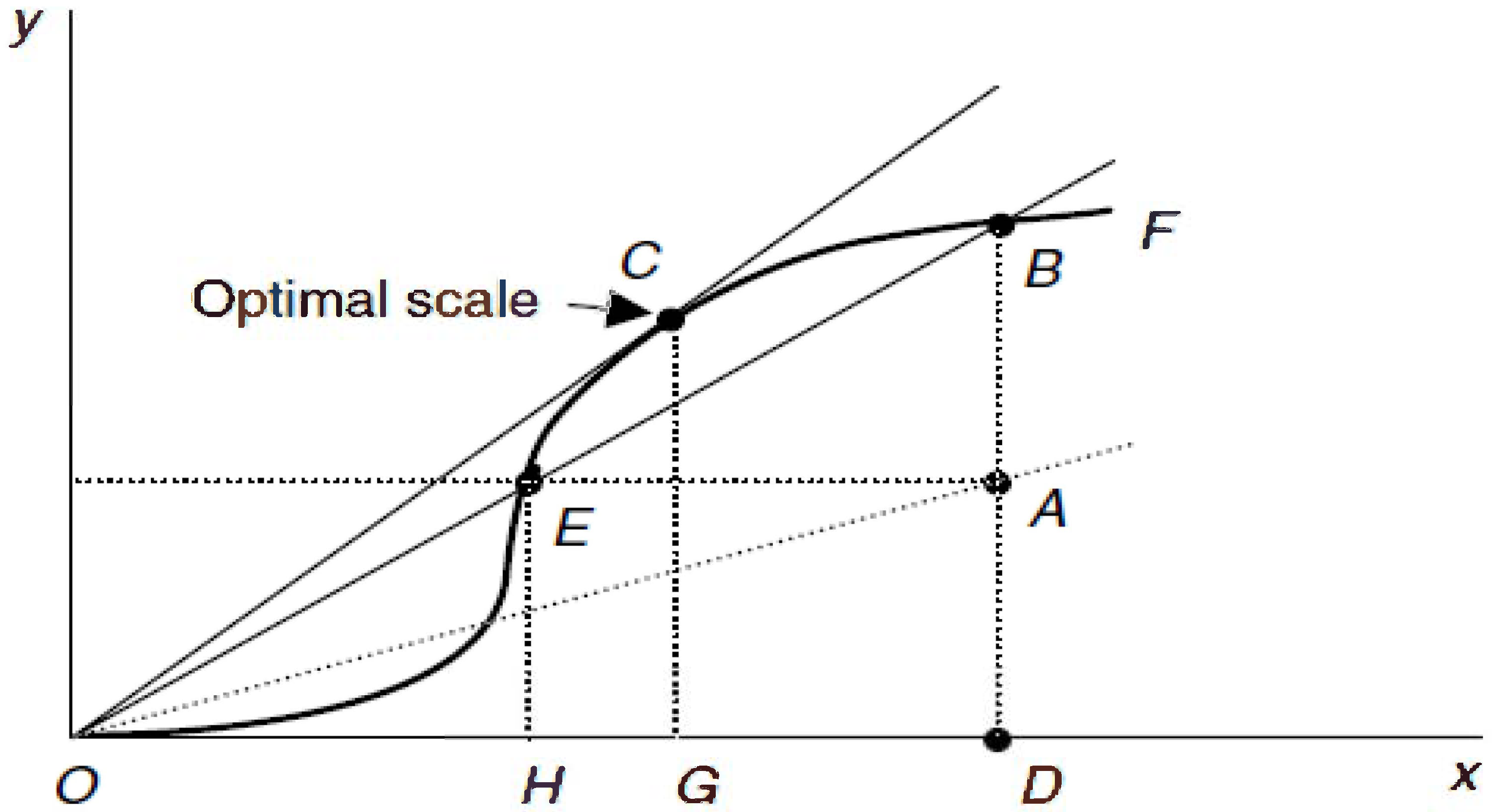
More often, productivity and efficiency are used interchangeably. Productivity is the rate at which a corporation produces outputs per unit of input or the quantity produced about the number of resources required to generate them. On the other hand, efficiency can be defined as completing a task without wasting resources or using fewer resources, such as fertilizer, energy, and water [24]. Figure 2 shows the difference between productivity and efficiency for a single-input–single-output case.

In Figure 2, three distinct producers are denoted as points A, B, and C. At point A, productivity is determined by the output ratio, $DA$, to the input, $OD$, expressed as $productivity=\frac{DA}{0D}$. To gauge productivity at a specific point, a ray originating from the origin can be used, and its slope, represented by $\frac{y}{x}$, indicates the productivity level at that point. For instance, if a firm moves from point A to point B, it becomes more productive, as the slope of the ray from the origin to point B exceeds that from the origin to point A. At point B, however, the firm is technically more efficient than at point A, operating on the production function curve. Shifting to point C, and the ray from the origin becomes tangent to the production frontier curve, making point C the location of the highest potential productivity using scale economies. Point C is also at the technically optimum scale since, at this point, the slope of productivity matches the slope of the production frontier curve. Other positions on the graph above indicate poorer performance in productivity and efficiency [25]. Despite using the same input, transitioning from point A to point B could further enhance productivity. To evaluate the efficiency of point A, the ratio of point A’s productivity to that of point B is considered, i.e., $efficiency=\left(\frac{DA}{0D}\right)/\left(\frac{DB}{0D}\right)=\frac{DA}{DB}$ [25].

This efficiency is commonly referred to as technical efficiency ($TE$) and encompasses both output and input technical efficiencies. In simpler terms, a producer can enhance output using the same inputs (illustrated by output-oriented items A–B) or reduce input while maintaining the same output through technological improvements (depicted by input-oriented items A–E). Consequently, the curve $OF$ in Figure 2 signifies the production frontier, wherein all points located on it are technically efficient. Conversely, points situated below the production frontier indicate technical inefficiency [24].

Measuring productivity and efficiency is critical for assessing the production units for the performance of various sectors or the general performance of the whole economy. This allows for identifying the causes and effects of efficiency and productivity differentials, which is critical for future policies to enhance the producer performance. For instance, measuring productivity and efficiency can teach the producers about the inputs used in the production process to increase their productivity concerning the farm’s performance in specific sectors and for various sectors [26]. The departure from the frontier function determines the technical efficiency of an individual production unit. Because this frontier function is challenging to know in reality, it must be calculated from a sample of observed production units for the inputs used in the production process. Furthermore, technical efficiency assessments are usually performed using frontier methods, which move the average response functions to the maximum output or the most efficient company [26].

According to Lovell et al. [27], two principal methodologies were utilized to estimate the frontier function: data envelopment analysis (DEA), which uses nonparametric linear programming, and stochastic frontier analysis (SFA), which employs parametric econometric estimation. This paper follows the SFA estimation methodology using the production function. Following Aignet et al. [28], a Cobb–Douglas production stochastic frontier relates the output y to a vector of input x, and technical inefficiency u for a production unit i as

$$ln{y}_i=x_i^{\prime }\beta -u_{i}fori=1,2,\dots N,and{u}_i\ge 0$$

(1)

where ln is the natural logarithm function, and N is the number of production units. Aigner et al. [29] and Meeusen et al. [30] modified the model in Equation (1) to include the random symmetric error ${}_{v}i$ to account for statistical noise due to measurement and approximation related to the functional form selection, omitted variables, such as weather and luck, which are not under the control of the production units [31]. The resulting model is the stochastic frontier analysis model because it includes both error terms: the technical inefficiency $u_i$ that might affect production due to fluctuations in many parameters and the typical random shock $v_i$. In the context of panel data, the stochastic frontier model becomes:

$$ln{y}_{it}=x_{it}^{\prime }\beta +v_{it}-u_{it}fori=1,2,\dots N,t=1,2,\dots ,Tand{u}_{it}\ge 0$$

(2)

The ratio of the output observed for the $i^{th}$ company compared to the prospective output specified by the frontier function determines the technical efficiency as follows

$$T{E}_{it}=\frac{exp\left(x_{it}^{\prime }\beta +v_{it}-u_{it}\right)}{exp\left(x_{it}^{\prime }\beta +v_{it}\right)}=exp\left(-u_{it}\right)with{u}_{it}\ge 0$$

(3)

The panel data stochastic frontier model in Equation (3) has two common versions of measuring efficiency and estimating the technical inefficiency factor: time-invariant and time-variant technical efficiency. The first implies that the technical inefficiency of individual producers remains constant throughout time, whereas the second allows for variation in inefficiency throughout time [32]. In this paper, we allow the TE to be a time-variant. In addition, $u_{it}$ can depend on variables, $z_{it}$, that can vary over time and across production units and affect their efficiency according to the following expression

$$u_{it}=z_{it}^{\prime }\delta +d_{it},$$

(4)

where $d_{it}$ is a random variable with an assumed distribution, and $\delta$ are unknown parameters to be estimated. Furthermore, we assume that the inefficiency component $u_{it}$ can follow the half-normal, the exponential, the truncated normal, and the Gamma distribution.

3. Data and the Empirical Estimation

This section consists of two parts. The first part describes the data employed in this analysis: data source, descriptive statistics, and some background regarding crop production across some European countries. The second part gives the estimation strategy, including production model specification, inefficiency distribution specification, variable selection, and model selection using Vuong’s test [7].

3.1. Data

This paper uses two sets of data. The first set consists of annual barley, common wheat, and maize production and input use in some European Union countries. In addition, this set also contains some policy variables, such as subsidies. The annual data are publicly available on the official website of the Farm Accountancy Data Network (FADN) of the European Commission (we retrieved the data on 5 March 2023 from this website https://agridata.ec.europa.eu/extensions/DashboardFarmEconomyFocusCrops/DashboardFarmEconomyFocusCrops.html). The second set consists of macroeconomic variables such as GDP, inflation, and employment rate, which are publicly available on the World Bank’s official website. Both datasets span the period from 2008 to 2018.

Table 1. Summary statistics of variables used in SFA.

Variables	Mean	Std.	Min	Max
Barley
Total output (tons)	3991.24	3786.74	254.4	13,098.23
Total utility area (ha)	849.55	773.36	102.48	3486.9
Quantity index of fertilizer	1101.13	1041.85	57.44	4414.22
Price index for fertilizer	108.205	16.26	73.8	165.3
Quantity index of seed	477.91	410.43	37.32	1946.18
Price index for seed	106.147	10.601	77.9	141.2
Quantity index of machine and lubricants	608.44	532.93	59.55	2028.68
Machine and building upkeep (EUR 1000)	59,814.99	60,966.33	543.55	301,548.98
Price index for machine and lubricants	104.162	14.169	69.2	138.1
Quantity index of energy	104.49	104.9	0.73	550.54
Price index for energy	104.375	10.126	73.3	127
Interest payment (1000 EUR/ha)	0.03	0.05	0	0.29
Contract work (1000 EUR)	49,479.82	49,076.64	6.16	286,565.58
Rent payment (1000 EUR/ha)	0.05	0.03	0	0.18
Wage payment (1000 EUR/ha)	0.02	0.02	0	0.15
Total labor input (AWU)	891.37	906.74	77.26	3553.7
Quantity index of crop protection	595.92	715.06	5.1	3164.08
Own capital cost (1000 EUR/ha)	0.11	0.07	0	0.42
Family labor costs (1000 EUR/ha)	0.28	0.19	0	1.17
Wheat
Total output (tons)	6625.67	8781.73	298.63	40,944.64
Total utility area (h)	1153.31	1210.36	107.6	5161.39
Quantity index of fertilizer	1820.29	2410.15	109.64	12,029.78
Price index for fertilizer	108.725	15.921	73.8	165.3
Quantity index of seed	780.63	902.6	44.13	4591.1
Price index for seed	106.285	10.667	77.9	145.6
Quantity index of machine and lubricants	926.7	948.51	57.31	3780.6
Price index for machine and lubricants	104.608	14.739	64.1	166.4
Machine and building upkeep (EUR 1000)	74,964.95	99,700.05	2649.19	457,612.55
Quantity index of energy	124.37	137.04	2.91	585.07
Price index for energy	104.023	11.056	68.2	142.7
Interest payment (1000 EUR/h)	0.01	0	0.01	0.02
Contract work (EUR 1000)	72,876.04	102,306.59	1009.53	498,018.12
Rent payment (1000 EUR/h)	0.01	0	0.01	0.02
Wage payment (1000 EUR/h)	0.01	0	0.01	0.02
Total labor input (AWU)	1819.73	1938.85	11.7	7503.38
Quantity index of crop protection	1419.24	2366.55	1.4	11,278.72
Own capital cost (1000 EUR/h)	0.01	0	0.01	0.01
Family labor costs (1000 EUR/h)	0.02	0	0.01	0.02
Maize
Total output (tons)	4529.62	4272.51	226.63	18,663.94
Total utility area (h)	628.21	674.66	36.39	2731.16
Quantity index of fertilizer	1075.36	1086.94	27.56	5243.49
Price index for fertilizer	109.05	13.724	76.44	165.3
Quantity index of seed	763.27	773.64	5.3	3253.04
Price index for seed	105.344	9.144	77.9	136.24
Quantity index of machine and lubricants	667.27	589.92	24.56	1988.87
Price index for machine and lubricants	104.363	14.635	64.1	166.4
Machine and building upkeep (EUR 1000)	38,976.17	47,687.85	2351.37	237,548.72
Quantity index of energy	174.07	235.93	0.53	1344.85
Price index for energy	104.206	10.839	68.2	142.7
Interest payment (1000 EUR/h)	0.01	0	0.01	0.02
Contract work (EUR 1000)	62,662.30	76,312.84	536.43	370,289.15
Rent payment (1000 EUR/h)	0.01	0	0.01	0.02
Wage payment (1000 EUR/h)	0.01	0	0.01	0.02
Total labor input (AWU)	796.76	856.17	19.19	4191.12
Quantity index of crop protection	552.76	595.31	26.57	2600.25
Own capital cost (1000 EUR/h)	0.01	0	0.01	0.01
Family labor costs (1000 EUR/h)	0.02	0	0.01	0.02

presents the summary statistics of the variables used in the production function at the aggregate level and the price indexes for energy, fertilizer, seeds, and machine and lubricants used to define the quantity index for each of these variables (the total expenditure of any variable for each year divided by the price index of the same year), aggregated across all countries. Detailed descriptive statistics are available upon request.

We notice that the machine, building upkeep, and contract work have the highest expenditure for barley with EUR 59,814.99 and EUR 49,479.82, respectively. Comparatively, wage payment and own capital costs are only 0.02 EUR/ha and 0.11 EUR/ha, respectively. We observe the same pattern for common wheat, with an average of 1.39 EUR/ha on capital costs. On the other hand, growing maize seems to cost less in terms of machine and building upkeep, with EUR 38,976.17. However, the contract work and own capital costs are similar to those for the common wheat.

Table 2. Summary statistics of macroeconomic and subsidies variables used in crops production.

Technical Inefficiency Variable	Mean	Std. Dev.	Min.	Max.
Agriculture value added (% of GDP)	2.402	1.171	0.558	6.302
Total unemployment (%)	9.604	4.765	2.24	27.47
Employment in agriculture—female (%)	5.198	6.089	0.55	32.36
Employment in agriculture—male (%)	7.665	5.31	1.38	29.95
Employment in industry—male (%)	36.408	6.795	19.93	52.48
Employment in industry—female (%)	14.602	5.294	6.91	28.63
Exports of goods and services (annual % growth)	3.967	7.169	−20.309	39.25
Exports of goods and services (% of GDP)	53.463	22.51	18.982	122.99
Imports of goods and services (annual % growth)	3.012	8.304	−30.894	32.448
Imports of goods and services (% of GDP)	51.699	19.24	23.02	105.859
Foreign direct investment (%)	3.685	8.822	−40.33	81.335
GDP growth (%)	1.249	3.835	−14.839	25.176
Industry, value added (% of GDP)	24.335	5.06	13.226	38.695
Inflation (annual %)	1.761	2.183	−9.728	16.016
Total labor force (1 million)	10.034	11.912	0.676	43.562
Population growth (annual %)	0.031	0.671	−2.258	2.039
Total population (1 million)	20.746	24.395	1.315	82.906
Urban population (%)	69.634	10.62	52.209	87.874
Rural population (%)	30.366	10.62	12.126	47.791
Agricultural land (% of land area)	43.481	16.891	7.387	73.096
Forest area (% of land area)	0.693	0.741	0.058	2.809
Wage and salaried workers—male (%)	80.583	6.706	59.49	89.27
Wage and salaried workers—female (%)	87.652	6.775	65.63	95.02
Total direct payments (EUR 1000)	16.68	19.836	0.1	83.616
Total subsidies on crops (EUR 1000)	0.815	2.093	0	17.151
Total subsidies on livestock (EUR 1000)	0.339	1.014	−0.002	5.883
Total support for rural development (EUR 1000)	2.403	3	0.002	13.819
Subsidies on intermediate consumption (EUR 1000)	0.597	1.302	0	5.859
Decoupled payments (EUR 1000)	14.733	18.504	0.09	81.799
Other subsidies (EUR 1000)	0.918	1.933	0	11.897

presents statistical summaries across all countries of the macroeconomic and agricultural policy variables used to explain the inefficiency. The detailed summary statistics for each country in this study are available upon request.

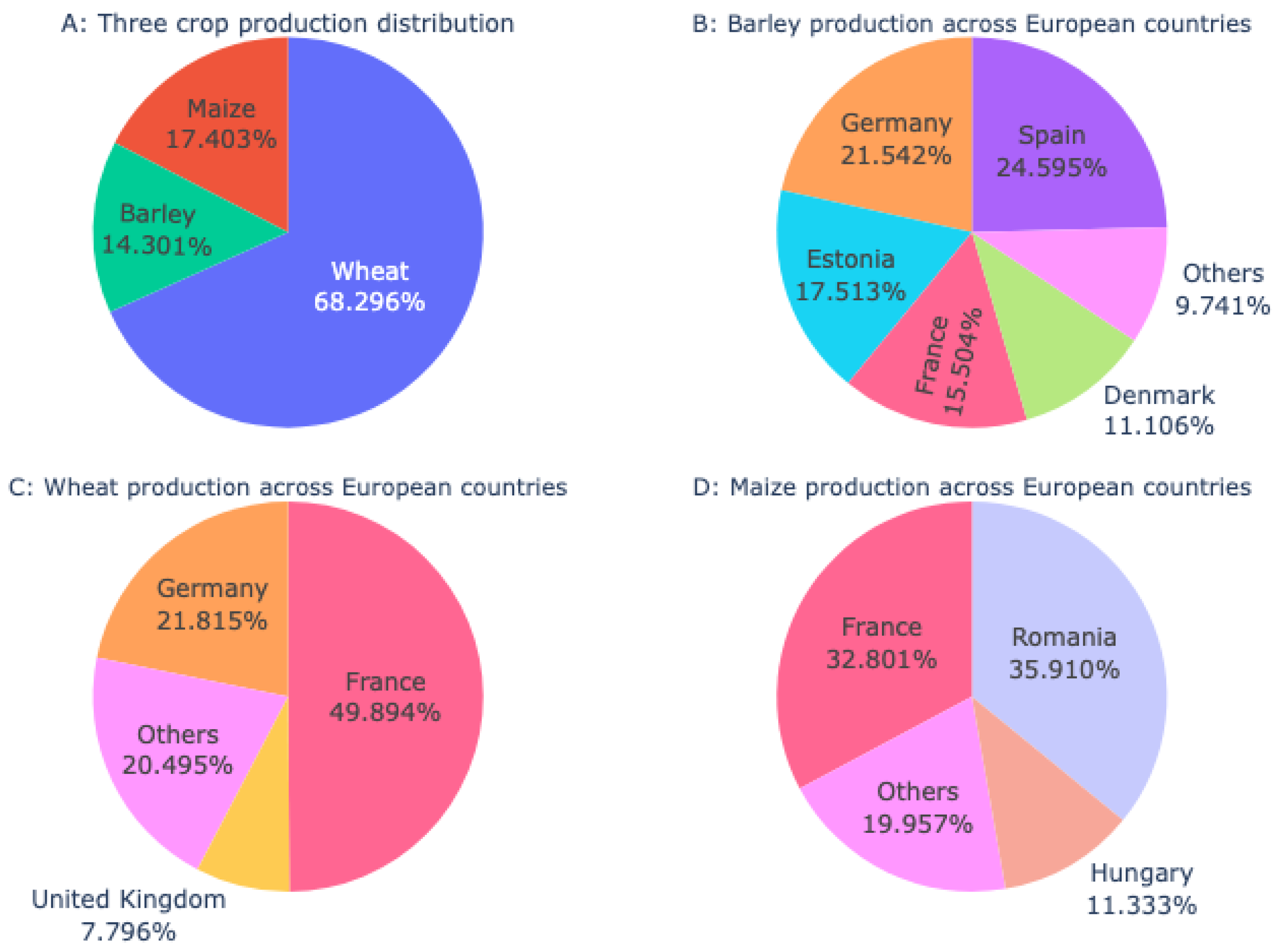
Figure 3 provides a snapshot of the barley, grain maize, and wheat output distribution for the European countries included in this study. The percentages are for the total production of the three crops. Hence, in Figure 3A, common wheat, barley, and maize represent 14%, 18%, and 68% of the total output from these crops across all the countries considered. When we consider barley, Figure 3B shows that Spain, Germany, and France are the top producers, with 25%, 22%, and 15% for each. On the other hand, the least producers are Sweden, Romania, Italy, and Ireland, producing roughly 1%, 1%, 0.1%, and 0.2%, respectively, of the total barley across the considered countries. For maize, Figure 3D indicates that France and Romania produce around 33% and 36% of the total production for each, respectively.

In contrast, Slovenia, Slovakia, and Portugal have the lowest grain maize production levels among European countries in the study. Regarding wheat production, Figure 3C shows that France has the highest production level with 50%, while the other countries have almost the same production level share of between 0.1 and 8%.

3.2. Estimation Strategy

The estimation strategy proceeds in three steps. First, we perform a random forest regression, a machine learning technique, to identify the variables for the production (Equation (2)) and inefficiency (Equation (4)) models. We justify using the random forest regression technique by saving on the degrees of freedom given the high number of explanatory variables in both models and the small sample size. In the second step, we estimate the production frontier using the identified covariates from the first step under three distributional assumptions: half-normal, exponential, and truncated normal distributions. Finally, we use the Vuong (1989) test to identify which model best fits the data.

3.2.1. Random Forest Regression

Random forest is an ensemble technique described as a modification of bagging or bootstrapping aggregation used for classification and regression (Bagging or bootstrapped aggregation is a machine learning technique involving multiple iterations of bootstrapping and training an estimation for each bootstrapped sample.). The random forest technique has been shown to demonstrate exceptional prediction performance on various benchmark datasets [33]. First, the random forest builds a series of decision trees for classification (data with discrete labels on the outcome variable). Then, it combines them using the average to obtain accurate results with low bias and low variance consistent with the actual dataset. In cases with a continuous outcome variable, the algorithm still builds many decision trees but bases the final decision on the average of all trees instead of a majority voting. The idea of the random forest technique is to reduce the level of variance by averaging the noise without randomization. For the mathematics of the random forest model, see [34]. The process of the random forest technique proceeds in four steps:

• Randomly choose samples from the training dataset with replacements;
• Grow a decision in each sample from step 1;
• Choose the optimal split at each node among the randomly q predictors out of a total of p predictors. The user may set the number of q predictors;
• Repeat the steps (1–3) until the T trees are grown.

Once we have T trees, we use the aggregation techniques for a final estimate. One of the random forest model outcomes is the variable importance measure, obtained using the mean decrease impunity (MDI) algorithm. For estimation, we use the RandomForestRegressor algorithm from the Python package sklearn.

3.2.2. Stochastic Frontier under Different Distributions

This research explores the production of three cereal products in various European countries, utilizing the general panel Cobb–Douglas production function specification and analyzing three distinct distributions: half-normal, exponential, and truncated normal (the translog specification was not considered due to the limited sample size). The technical inefficiency model of Equation (4) consists of macroeconomic factors like inflation, GDP, and unemployment rate, as well as agricultural policies such as total crop subsidies, total livestock subsidies, total rural development support, decoupled payments, intermediate consumption subsidies, and other subsidies offered by certain European countries. For estimation, we use the command frontier from the STATA 15 software.

3.2.3. Testing between Different Specifications: Vuong’s Test

In general, Vuong’s test [7] compares non-nested models. Non-nested models can be identified as having two or more models (or hypotheses) that can neither be derived from the other through acceptable parametric constraints nor as a limit of a reasonable approximation [35]. Furthermore, Vuong’s test provides the economist with the information necessary to identify the optimal model under the various assumptions by testing the null hypothesis in Equation (5):

$$lnL\left(modelj\right)-lnL\left(modelk\right)=0$$

(5)

against the alternative hypothesis in Equation (6)

$$lnL\left(modelj\right)-lnL\left(modelk\right)>0,$$

(6)

where $modelj$ and $modelk$ are any two competing models, and $lnL$ is the log-likelihood function. Equation (7) provides the Vuong statistic as

$$V=\frac{\sqrt{n}\left(\frac{1}{n}{\sum }_{i=1}^n{m}_i\right)}{\sqrt{\frac{1}{n}{\sum }_{i=1}^n{\left(m_i-\overline{m}\right)}^2}},$$

(7)

where $m_i=lnL\left(mode{l}_{i,j}\right)-lnL\left(mode{l}_{i,k}\right)$ and $\overline{m}$ is the average of $m_i$.

Vuong [7] has shown that V has an asymptotic standard normal distribution if the two models are equivalent. In contrast, if V tends towards positive infinity, then $mode{l}_j$ fits the data better than $mode{l}_k$. Finally, $mode{l}_k$ outperforms $mode{l}_j$ if V goes to negative infinity.

4. Results and Discussion

This section will first present the random forest regression estimation results. This step will help us choose the most important variables to estimate the production function and the inefficiency equation. Next, we will provide the SFA estimation results under three distributions: half-normal, truncated normal, and exponential. After that, we will present the pairwise Vuong test results to identify the model that best suits the data for each crop. Finally, we will discuss the results of the best model.

4.1. Random Forest Regression Results

In this research, we employed random forest regression to identify the key explanatory variables for estimating the production and inefficiency equations. We utilized the RandomForestRegressor algorithm from the popular sklearn library in Python to estimate variable importance. Breiman [33] defines variable importance as the increase in prediction error resulting from removing a specific variable from the predictors. Before using the importance scores, we performed model validation by splitting the sample into training (75%) and testing (25%) sets, used the root mean absolute percentage error (MAPE), and computed the model accuracy by subtracting the mean MAPE from 100. The accuracy measures ranged from 89.77% for truncated normal distribution for barley to 93.23% for half-normal distribution for wheat. We presented the variable importance results of the random forest in

Table 3. Random forest regression for the production function.

Variables	Importance Score
Barley inputs
Total utility area (ha)	0.6733
Quantity index of fertilizer	0.1884
Quantity index of seed	0.0499
Rent payment (EUR/ha)	0.0358
Quantity index of crop protection	0.0111
Quantity index of machine and lubricants	0.0104
Common wheat input
Total utility area (ha)	0.6739
Quantity index of seed	0.1032
Quantity index of crop protection	0.0593
Rent payment (EUR/ha)	0.0578
Own capital cost (EUR/ha)	0.0231
Quantity index of energy	0.0228
Grain maize inputs
Quantity index of seed	0.6672
Total utility area (ha)	0.1772
Family labor costs (EUR/ha)	0.0266
Contract work (EUR/ha)	0.0262
Rent payment (EUR/ha)	0.0156
Quantity index of machine and lubricants	0.0150

for the production function and

Table 4. Random forest importance score for variables entering technical inefficiency.

Variables	Importance Score
Barely
Half-normal distribution
Agriculture value added (% of GDP)	0.3309
Employment in industry—male (%)	0.0973
Agricultural land (% of land area)	0.0445
Wage and salaried workers—female (%)	0.0329
Foreign direct investment (%)	0.0299
Inflation (annual %)	0.0267
Exponential distribution
Agriculture value added (% of GDP)	0.3055
Employment in industry—male (%)	0.1027
Agricultural land (% of land area)	0.0478
Foreign direct investment (%)	0.0448
Employment in agriculture—female (%)	0.0341
Forest area (% of land area)	0.0341
Truncated normal distribution
Agriculture value added (% of GDP)	0.3315
Employment in industry—male (%)	0.0973
Agricultural land (% of land area)	0.0447
Wage and salaried workers—female (%)	0.0329
Foreign direct investment (%)	0.0301
Inflation (annual %)	0.0266
Common wheat
Half-normal distribution
Total unemployment (%)	0.0955
Decoupled payments (EUR)	0.0937
Wage and salaried workers—male (%)	0.0822
Agriculture value added (% of GDP)	0.0712
Forest area (% of land area)	0.0701
Employment in agriculture—male (%)	0.0437
Exponential distribution
Total unemployment (%)	0.1273
Wage and salaried workers—male (%)	0.1046
Forest area (% of land area)	0.0639
Other subsidies (EUR)	0.0576
Agricultural value added (% of GDP)	0.0525
Decoupled payments (EUR)	0.0462
Truncated normal distribution
Total unemployment (%)	0.0876
Agricultural value added (% of GDP)	0.0830
Decoupled payments (EUR)	0.0829
Forest area (% of land area)	0.0826
Wage and salaried workers—male (%)	0.0718
Employment in agriculture—male (%)	0.0437
Variables	Importance score
Grain maize
Half-normal distribution
Employment in industry—female (%)	0.3549
Total unemployment (%)	0.099
Industry, value added (% of GDP)	0.0521
Forest area (% of land area)	0.0392
Other subsidies (EUR)	0.0358
Employment in agriculture—male (%)	0.0311
Exponential distribution
Employment in industry—female (%)	0.1985
Total unemployment (%)	0.1205
Industry, value added (% of GDP)	0.0903
Employment in industry—male (%)	0.0530
Forest area (% of land area)	0.0512
Exports of goods and services (annual % growth)	0.0397
Truncated normal distribution
Employment in industry—female (%)	0.2577
Total unemployment (%)	0.1175
Industry, value added (% of GDP)	0.0903
Industry, value added (% of GDP)	0.0799
Forest area (% of land area)	0.0426
Employment in industry—male (%)	0.0402
Exports of goods and services (annual % growth)	0.0367

for the technical inefficiency estimation under various distributional assumptions.

Our findings on barley reveal that the most significant variables that explain the variation in barley production are the total utility area, quantity of fertilizer, amount of seed, rent payment, crop protection, and machine and lubricants, contributing 67.33%, 18.84%, 4.99%, 3.58%, 1.11%, and 1.04%, respectively. These six variables together account for approximately 96% of the barley production variation. Consequently, we retained these six variables to estimate the production function under diverse technical inefficiency distributional assumptions.

Regarding common wheat, based on the random forest analysis, the largest contributor to the variation in output is the total utility area, which accounts for 67.39%. Other variables, such as seed quantity, crop protection, rent payment, cost of own capital, and amount of energy, explain smaller percentages in the variation (10.32%, 5.93%, 5.78%, 2.31%, and 2.28%, respectively). Due to collinearity issues, we excluded the cost of own capital and the quantity of energy and instead included machine and building upkeep expenses. With these changes, the specification now explains approximately 91% of the total variation in wheat production.

For grain maize, the random forest variable importance analysis indicates that the largest contributors to the variation in output are the seed quantity, total area, expenditure on contract work, rent payment, and machine and lubricants quantity, which account for roughly 93%. However, due to multicollinearity, we removed the expenditure on family labor and added the expenditure on crop protection instead.

The random forest regression analysis findings are displayed in Table 4, examining the impact of various macroeconomic and agricultural policies on barley output as technical inefficiency factors. The analysis was conducted under three distributional assumptions. The results suggest that the percentage of agriculture value added in GDP is the most significant factor affecting the technical efficiency of barley crops, accounting for 33.09%, 30.55%, and 33.15% of the total variation for half-normal, exponential, and truncated normal distributions, respectively. Conversely, the intermediate consumption subsidies are the least important factor, contributing only 1.49% and 1.32% of the total variation under half-normal and truncated normal distributions, respectively. However, for the exponential distribution, total direct payments are the least significant factor, accounting for approximately 1.15% of the total variation in technical efficiency.

Table 4 displays the random forest regression analysis results for technical inefficiency variables of the common wheat crop using three distributions: half-normal, exponential, and truncated normal. The analysis reveals that the unemployment rate (as a percentage of the labor force) is the most significant predictor of the total technical efficiency for common wheat. It accounts for 9.55%, 12.73%, and 8.76% of the total variation in technical efficiency under the three distributions, respectively. Conversely, the imports of goods and services (as a percentage of GDP) have the least impact on the common wheat crop, accounting for only 1.05%, 1.02%, and 1.07% of the total variation in technical efficiency under the three distributions.

The study found that female employment in the industry sector is the most crucial variable in predicting the technical efficiency of grain maize. This variable accounts for 35.49%, 19.85%, and 25.77% for half-normal, exponential, and truncated normal distributions, respectively (refer to Table 4 for details). On the other hand, the least important variable varies based on the distribution used. For example, the variable exports of goods and services (as a proportion of GDP) is the least important variable under the half-normal distribution. In the exponential distribution, the total population accounts for approximately 0.85% of the technical efficiency variation. Finally, under the truncated normal distribution, the total labor force accounts for around 0.94% of the total variation in the technical efficiency of grain maize. To sum up, it is important to note that the random forest variable importance provides a ranking of the relevant variables. However, this ranking may be deviated from when some variables have multicollinearity issues.

4.2. Stochastic Frontier Analysis Results

Table 5. Stochastic frontier results for barley.

Variable	Half-Normal	Exponential	Truncated Normal
Production function
Intercept	2.125 ***	1.862 ***	2.782 ***
	(0.233)	(0.256)	(0.234)
Total utility (ha)	0.835 ***	0.809 ***	0.863 ***
	(0.043)	(0.052)	(0.049)
Quantity index of seed	−0.122 ***	−0.099 ***	−0.098 ***
	(0.045)	(0.053)	(0.039)
Quantity index of fertilizer	0.207 ***	0238 ***	0.092 *
	(0.047)	(0.049)	(0.047)
Rent payment (EUR/ha)	0.203 ***	0.177 ***	0.125 ***
	(0.018)	(0.021)	(0.031)
Quantity index of crop protection	0.139 ***	0.134 ***	0.091 **
	(0.022)	(0.026)	(0.036)
Quantity index of machine and lubricants	−0.153 ***	−0.155 ***	−0.056
	(0.041)	(0.042)	(0.042)
Technical inefficiency
Intercept	28.976 **	56.422 **	7.431 ***
	(13.094)	(21.951)	(1.565)
Employment in industry—male (%)	−0.114	-	0.011 *
	(0.088)	-	(0.007)
Wage and salaried workers—female (%)	−0.807 ***	−1.259 ***	−0.126 ***
	(0.259)	(0.437)	(0.026)
Foreign direct investment (%)	−0.065 *	−0.094	−0.009 *
	(0.039)	(0.072)	(0.005)
Forest area (% of land area)	1.482 ***	1.654 *	-
	(0.396)	(0.971)	-
Employment in agriculture—female (%)	−0.71 ***	−0.657 ***	−0.058 ***
	(0.202)	(0.242)	(0.014)
Other subsidies (EUR)	0.498 *	0.339	−0.002
	(0.278)	(0.405)	(0.03)
Industry, value added (% of GDP)	−0.062	-	−0.001
	(0.072)	-	(0.009)
Employment in industry—female (%)	0.546 **	0.188	-
	(0.238)	(0.166)	-
Total labor force	−0.073 **	-	-
	(0.032)	-	-
Employment in agriculture—male (%)	0.385 **	-	-
	(0.194)	-	-
Wage and salaried workers—male (%)	0.235	0.585 **	0.051 ***
	(0.17)	(0.246)	(0.014)
Exports of goods and services (% of GDP)	0.088 ***	0.061 **	0.004 *
	(0.031)	(0.03)	(0.002)
Urban population (%)	0.198 **	-	-
	0.092	-	-
Total subsidies on crops (EUR)	0.16 *	-	0.008
	(0.091)	-	(0.01)
Inflation (annual %)	−0.079	-	-
	(0.11)	-	-
Imports of goods and services	0.007	-	-
	(0.019)	-	-
Agricultural land (% of land area)	-	0.019	−0.005 ***
	-	(0.037)	(0.002)
Total unemployment (%)	-	0.134 **	0.025 ***
	-	(0.056)	(0.005)
Total population	-	−0.092 ***	−0.01 ***
	-	(0.035)	(0.002)
Total support for rural development (EUR)	-	0.093	-
	-	(0.091)	-

(*): significance level at 10%; (**): significance level at 5%; and (***): significance level at 1%. Figures between parentheses are coefficient standard errors.

,

Table 6. Stochastic frontier results for common wheat.

Variable	Half-Normal	Exponential	Truncated Normal
Production function
Intercept	9.289 ***	10.347 ***	8.611 ***
	(1.642)	(1.657)	(2.233)
Total utility area (ha)	0.617 ***	0.538 ***	0.632 ***
	(0.046)	(0.046)	(0.056)
Quantity index of seed	0.07	0.141 ***	0.037
	(0.045)	(0.046)	(0.049)
Quantity index of crop protection	0.522 ***	0.587 ***	0.462 ***
	(0.09)	(0.093)	(0.122)
Rent payment (EUR/ha)	−5.101 ***	−5.734 ***	−4.379 ***
	(0.939)	(0.97)	(1.245)
Machine and building upkeep (EUR/ha)	0.171 ***	0.16 ***	0.167 ***
	(0.021)	(0.022)	(0.025)
Technical inefficiency
Intercept	1.583	3.313	−0.883
	(1.583)	(2.866)	(0.667)
Decoupled payments (EUR)	0.272	−0.023 *	0.037 *
	(0.186)	(0.012)	(0.019)
Total labor force	1.758 ***	-	0.187 ***
	(0.424)	-	(0.051)
Total direct payments (EUR)	−0.393 **	-	−0.053 ***
	(0.193)	-	(0.021)
Total population	−0.812 ***	-	−0.086 ***
	(0.198)	-	(0.023)
Employment in agriculture—female (%)	−0.37 ***	-	-
	(0.14)	-	-
Urban population (%)	0.075 **	-	0.02 ***
	(0.032)	-	(0.004)
Wage and salaried workers—male (%)	−0.202 ***	−0.105 ***	−0.105 ***
	(0.049)	(0.031)	(0.004)
Agriculture value added (% of GDP)	0.258	-	-
	(0.289)	-	-
Forest area (% of land area)	−0.412	-	0.138 **
	(0.515)	-	(0.068)
Total support for rural development (EUR)	0.067	-	-
	(0.104)	-	-
Employment in industry—male (%)	0.108 *	0.091 *	0.024 ***
	(0.06)	(0.054)	(0.009)
Employment in agriculture—male (%)	0.373 **	-	0.013 *
	(0.147)	-	(0.008)
Agricultural land (% of land area)	−0.041 *	−0.043 **	−0.005 *
	(0.022)	(0.017)	(0.003)
Total unemployment (%)	0.084 **	0.124 ***	0.024 ***
	(0.041)	(0.039)	(0.004)
Other subsidies (EUR)	0.308 *	-	0.037 *
	(0.187)	-	(0.021)
Industry value added (% of GDP)	0.125 *	-	0.007
	(0.075)	-	(0.008)
Imports of goods and services	−0.004	0.009	-
	(0.016)	(0.018)	-
Total subsidies on livestock (EUR)	-	0.545 *	0.11 ***
	-	(0.319)	(0.042)
Employment in industry—female (%)	-	−0.076	0.002
	-	(0.08)	(0.011)
Population growth	-	−0.632 *	-
	-	(0.379)	-
Foreign direct investment (%)	-	0.01	−0.001
	-	(0.038)	(0.003)

(*): significance level at 10%; (**): significance level at 5%; and (***): significance level at 1%. Figures between parentheses are coefficient standard errors.

and

Table 7. Stochastic frontier results for grain maize.

Variable	Half-Normal	Exponential	Truncated Normal
Production function
Intercept	−14.174 ***	−12.28 ***	−10.974 **
	(3.134)	(3.176)	(5.392)
Quantity index of seed	0.062 ***	0.077 ***	0.052 **
	(0.023)	(0.025)	(0.025)
Total utility area (ha)	0.888 ***	0.893 ***	0.917 ***
	(0.056)	(0.058)	(0.059)
Contract work	0.047	0.075 ***	0.008
	(0.029)	(0.027)	(0.035)
Rent payment (EUR/ha)	10.796 ***	9.416 ***	8.889 ***
	(2.077)	(2.100)	(3.363)
Quantity index of machine and lubricants	0.019	0.013	0.035
	(0.039)	(0.045)	(0.038)
Quantity index of crop protection	−0.896 ***	−0.823 ***	−0.741 ***
	(0.156)	(0.163)	(0.271)
Technical inefficiency
Intercept	13.391	6.261	3.429 *
	(11.414)	(15.188)	(1.769)
Employment in industry—female (%)	0.126	0.195 *	0.028 ***
	(0.077)	(0.112)	(0.01)
Employment in industry—male (%)	0.269 ***	0.294 ***	0.041 ***
	(0.08)	(0.100)	(0.013)
Employment in agriculture—male (%)	1.221 ***	1.505 ***	0.199 ***
	(0.294)	(0.395)	(0.051)
Total support for rural development (EUR)	0.615 **	0.546	0.068
	(0.311)	(0.36)	(0.048)
Employment in agriculture—female (%)	−1.185 ***	−1.438 ***	−0.195 ***
	(0.326)	(0.43)	(0.055)
Wage and salaried workers—male (%)	0.473 ***	0.644 ***	0.089 ***
	(0.158)	(0.228)	(0.028)
Wage and salaried workers—female (%)	−0.778 ***	−1.004 ***	−0.145 ***
	(0.257)	(0.371)	(0.046)
Agricultural land (% of land area)	−0.055 **	−0.069 **	−0.008 **
	(0.028)	(0.031)	(0.004)
Total direct payments (EUR)	−1.269	-	0.001
	(1.220)	-	(0.188)
Total subsidies on crops (EUR)	0.160	-	−0.122
	(1.590)	-	(0.215)
Other subsidies (EUR)	1.211	-	0.027
	(1.220)	-	(0.19)
Decoupled payments (EUR)	1.298	-	0.003
	(1.220)	-	(0.188)
GDP growth (annual %)	−0.124 *	−0.188	−0.017 **
	(0.070)	(0.122)	(0.008)
Total unemployment (%)	0.007	-	-
	(0.052)	-	-
Inflation (annual %)	0.090	0.121	-
	(0.104)	(0.151)	-
Agriculture value added (% of GDP)	-	−0.285	-
	-	(0.417)	-
Exports of goods and services (annual % growth)	-	0.044	-
	-	(0.05)	-
Foreign direct investment (%)	-	−0.012	-
	-	(0.032)	-
Total subsidies on livestock (EUR)	-	-	−0.053
	-	-	(0.284)

(*): significance level at 10%; (**): significance level at 5%; and (***): significance level at 1%. Figures between parentheses are coefficient standard errors.

show the maximum likelihood results of estimating the stochastic frontier for the three crops across the countries considered, along with the findings of the effect of macroeconomics and agricultural policy variables on technical inefficiency.

Table 5 displays the maximum likelihood estimation results of the stochastic frontier analysis and the impact of macroeconomic and policy variables on technical inefficiency for barley under three different distributions: half-normal, exponential, and truncated normal. Except for the quantity index of seed, machines, and lubricants, all coefficients exhibit statistical significance and align with the anticipated direction.

Assuming all other factors remain constant (ceteris paribus), the results indicate that a 1% increase in total utility area leads to a 0.835% increase in total barley production for the half-normal distribution. Similarly, a 1% increase in the fertilizer quantity index would result in a 0.207% increase in the overall barley production. Moreover, a 1% increase in rent payment and crop protection quantity index would increase the total barley production by 0.203% and 0.139%, respectively. However, a 1% rise in the seed quantity index reduces barley production by 0.122%, while a 1% increase in the quantity index of machines and lubricants will reduce the barley production by 0.153%.

Under the exponential distribution, a 1% increase in total utility area results in a 0.809% increase in overall barley production. Similarly, a 1% increase in the fertilizer quantity index would result in a 0.238% increase in the overall barley production. In contrast, a 1% increase in rent payment and crop protection quantity index resulted in 0.177% and 0.134% increases in the total barley production, respectively. However, a 1% rise in the seed quantity index lowers the barley production by 0.099%, while a 1% increase in the quantity index of machines and lubricants results in a 0.155% reduction in overall barley production.

Finally, under the truncated normal distribution, the results show that a 1% increase in total utility area enhances the overall barley production by 0.863%. Similarly, a 1% increase in the fertilizer amount index results in a 0.09% increase in barley production. Additionally, a 1% increase in rent payment and crop protection quantity index increased the total barley production by 0.125% and 0.091%, respectively. However, a 1% increase in the seed quantity index reduces barley production by 0.098%, while a 1% increase in the quantity index of machines and lubricants resulted in a 0.056% decrease in barley production.

Table 5 illustrates the influence of different macroeconomic and subsidy variables on the technical efficiency of barley production under three distributional assumptions. The findings indicate that certain variables significantly impact the overall technical efficiency of barley production, while others demonstrate no effect.

In the context of the half-normal distribution, factors such as male employment in the industry, industry value added as a percentage of GDP, male waged and salaried workers, inflation, and imports of goods and services exhibit no statistically significant impact on technical efficiency. Conversely, variables like female wage and salaried workers, female employment in agriculture, and the total labor force show a negative yet statistically significant effect on technical inefficiency. This suggests that these variables contribute to enhancing the technical efficiency of barley production.

Conversely, factors such as forest area, other subsidies, female employment in industry, male employment in agriculture, exports of goods and services as a percentage of GDP, urban population, and total crop subsidies demonstrate a statistically significant adverse impact on the technical efficiency of barley production. Furthermore, under the half-normal distribution, variables like male employment in industry, industrial value added as a proportion of GDP, male wages, inflation, and imports of goods and services do not exert a significant effect on technical efficiency and inefficiency in barley production.

In the context of exponential distribution, the findings indicate that female wages, female employment in agriculture, and the total population exhibit a statistically significant positive impact on the technical efficiency of barley production. Conversely, factors such as forest area, male wages, the total unemployment rate, and exports of goods and services as a percentage of GDP have a statistically significant adverse effect on the technical efficiency of barley production. Additionally, variables like foreign direct investment, other subsidies, female employment in the industry, total support for rural development, and agricultural land as a percentage of total land do not exert a significant influence on technical efficiency in barley production.

The regression analysis presented in Table 5 also examines the impact of macroeconomic and policy variables on technical efficiency within the truncated normal distribution. The results suggest that female wages, foreign direct investment, female employment in agriculture, agricultural land as a percentage of total land, and the total population demonstrate a statistically significant positive effect on the technical efficiency of barley production. Conversely, factors such as male employment in the industry, male wages, exports of goods and services as a percentage of GDP, and the total unemployment rate have a statistically significant negative impact on the technical efficiency of barley. Additionally, other subsidies, industry value added as a percentage of GDP, and total crop subsidies significantly influence the technical efficiency.

Table 6 illustrates the regression of frontier analysis and the influence of macroeconomic and policy variables on technical efficiencies for common wheat in some European Union member nations using the maximum likelihood estimator under the three distributional assumptions. The estimation results show that, except for the quantity index of seed under the half normal and truncated normal distribution, all inputs are statistically significant for wheat production. On a ceteris paribus basis, a 1% increase in total utility area results in a 0.617% increase in total wheat production under half-normal. Moreover, a 1% increase in the seed quantity index increases wheat production by 0.07%. Additionally, a 1% increase in the crop protection index results in a 0.522% increase in total wheat production. In comparison, a 1% increase in the machines and buildings’ upkeep yields a 0.171% increase in the total wheat production. However, a 1% increase in the rent payment, on the other hand, reduces the total wheat production by 5.101%.

The estimation under exponential distribution shows that increasing the total utility area by 1% boosts the overall wheat production by 0.538%. Besides that, increasing the seed quantity index by 1% increases the wheat production by 0.141%. Furthermore, increasing the quantity index crop protection by the same amount results in a 0.587% increase in total wheat production. In contrast, a 1% increase in rent payment resulted in a reduction in total wheat production of 5.734%. Additionally, a 1% increase in the machines’ and buildings’ upkeep implies a 0.16% increase in total wheat production.

Table 6 also provides the estimation results for the production frontier for the wheat under a truncated normal distribution. The results, ceteris paribus, reveal that a 1% increase in total utility area increases wheat production by 0.632%. At the same time, the same increase in the seed quantity index results in a 0.037% increase in total wheat production. Besides that, a 1% increase in the quantity index of crop protection yields a 0.46% increase in wheat production. However, raising the rent payment by 1% decreases the wheat production by 4.379%. The same increase in the machines and buildings’ upkeep resulted in a 0.167% decrease in the total wheat production.

Regarding the technical efficiency, Table 6 outlines the impact of various macroeconomic and subsidy factors on the technical efficiency of wheat production under different distributional assumptions. Several variables exhibit a statistically significant effect, while others show no discernible impact. For instance, within the half-normal distribution, total direct payments, total population, female wages, female agricultural employment, and agricultural land as a percentage of total land all exert a statistically significant positive influence on the technical efficiency of wheat production. Conversely, the total labor force, urban population, male employment in the industry, male employment in agriculture, total unemployment rate, other subsidies, and industry value added as a percentage of GDP demonstrate a statistically significant negative effect on the technical efficiency of wheat production. Furthermore, decoupled payments, agricultural value added as a percentage of GDP, forest area as a percentage of total land area, total support for rural development, and imports of goods and services for annual growth do not exhibit a significant influence on technical efficiency for wheat production under a half-normal distribution.

Furthermore, the results within the exponential distribution framework reveal that male wages, agricultural land as a percentage of total land, and annual population growth display a statistically significant positive impact on the technical efficiency of wheat production. Conversely, male employment in the industry, the overall unemployment rate, and total subsidies on livestock exhibit a statistically significant negative effect on the technical efficiency of wheat production. Additionally, the imports of goods and services, female employment in the industry, and foreign direct investment do not exert a significant influence on the technical efficiency of wheat production.

The regression outcomes presented in Table 6 further illustrate the impact of macroeconomic and policy variables on technical efficiency under the normal truncated distribution. The results reveal that total direct payments, total population, male wages, the forest area as a percentage of total land area, and agricultural land as a percentage of total land all exhibit a statistically significant positive effect on the technical efficiency of wheat production. Conversely, decoupled payments, the total labor force, urban population, male employment in the industry, male employment in agriculture, the total unemployment rate, other subsidies, and total subsidies on livestock demonstrate a statistically significant negative influence on the technical efficiency of wheat production. Furthermore, industry value added as a percentage of GDP, female employment, and foreign direct investment do not show a significant influence on the technical efficiency of wheat production.

Regarding the grain maize results, Table 7 provides the results of the SFA and inefficiency estimates. All inputs in grain maize production are statistically significant except for contract work, the quantity index of machines and lubricants under half-normal and truncated normal distributions, and the quantity index of machines and lubricants under the exponential distribution. According to this research, a 1% increase in the quantity index of seed under half-normal distribution results in a 0.062% increase in total grain maize production. At the same time, a 1% increase in total utility area results in a 0.888% increase in the total grain maize production. Furthermore, a 1% increase in contract work and rent payment increased grain maize production by 0.047% and 10.796%, respectively. The same increase in the quantity index of machines and lubricants will increase the grain maize production by 0.019%. However, a 1% increase in the crop protection quantity index reduces the output of grain maize by 0.896.

Additionally, under exponential distribution, the regression findings indicate that increasing the quantity index of seed by 1% increases the output of grain maize by 0.077%. Moreover, increasing the total utility area by 1% increases the grain maize production by 0.893%. Furthermore, increasing contract work, rent payment, and the quantity index of machines and lubricants by 1% improves grain maize production by 0.075, 9.416, and 0.01%, respectively. In comparison, a 1% increase in the quantity index of crop protection leads to a 0.82% decrease in grain maize production.

For the regression under a truncated normal distribution, the results indicate that a 1% increase in the quantity index of seed enhances the grain maize production by 0.05%. Similarly, a 1% increase in total utility area enhances it by 0.917%. Furthermore, increasing the contract work by 1% will increase the grain maize output by 0.008%. Furthermore, an increase in rent payment and machine lubricant quantity index by 1% will increase overall grain maize production by 8.889% and 0.035%, respectively. Finally, a 1% increase in the crop protection quantity index will reduce the grain maize production by 0.741%.

Concerning the estimation of the inefficiency equation, Table 7 delineates the impact of various macroeconomic and subsidy variables on the technical efficiency of grain maize production under different distributional assumptions. Most variables exhibit a statistically significant effect, while others show no discernible impact. For instance, within a half-normal distribution, male employment in the industry, male employment in agriculture, total support for rural development, and male wages all demonstrate a statistically significant positive effect on the technical efficiency of grain maize production. However, female employment in agriculture, female wages, agricultural land as a percentage of total land, and GDP all reveal a statistically significant negative effect on the technical efficiency of grain maize production. Furthermore, female employment in the industry, total direct payments, total subsidies on crops, other subsidies, decoupled payments, the total unemployment rate, and inflation do not exhibit a significant effect on the technical efficiency of grain maize production.

In the context of exponential distribution, male wages, female employment in the industry, male industry employment, and male employment in agriculture all exhibit a statistically significant positive impact on technical efficiency. Furthermore, employment in agriculture and female wages demonstrate a statistically significant negative influence on the technical efficiency of grain maize production. Additionally, the total rural development support, male wages, GDP annual growth, inflation, agricultural value added as a percentage of GDP, exports of goods and services, annual growth, and foreign direct investment do not have a significant effect on the technical efficiency of grain maize production.

Under truncated normal distribution, the results reveal that male employment in agriculture, male wages, female employment in the industry, and male employment in the industry significantly positively affect the overall technical efficiency of grain maize production. However, female employment in agriculture, agricultural land as a percentage of total land, GDP annual growth, and female wages significantly negatively impact the technical efficiency of grain maize production. Moreover, total support for rural development, total direct payment, total subsidies on crops, other subsidies, decoupled payments, and total subsidies on livestock do not have a significant effect on the technical efficiency of grain maize production.

4.3. Vuong Test Results

In this part, we report the results of Vuong’s test to compare the non-nested models. We carry this test for each crop.

Table 8. Vuong test results.

Barley
Null hypothesis	Vuong statistic	Distribution retained
Half-normal equivalent to exponential	17.368	Half-normal
Half-normal equivalent to truncated normal	24.069	Half-normal
Common wheat
Null hypothesis	Vuong statistic	Distribution retained
Half-normal equivalent to exponential	25.684	Half-normal
Half-normal equivalent to truncated normal	23.804	Half-normal
Gain maize
Null hypothesis	Vuong statistic	Distribution retained
Half-normal equivalent to exponential	24.113	Half-normal
Half-normal equivalent to truncated normal	20.918	Half-normal

If $-1.96<V<1.96$, the two models are equivalent. If $V>1.96$, the first model outperforms the second. If $V<-1.96$, the second model outperforms the first.

provides the pairwise comparison between the three distributional specifications. Given that the half-normal model outperforms the two other models, we conclude that the estimation under half-normal fits the data better for the three crops considered. In what follows, we will limit our discussion of the results implied by half-normal distribution.

4.4. Efficiency Results

When averaging across all countries and years, the estimates for barley’s technical efficiency scores range from 0.803 under the half-normal distribution to 0.835 under the exponential distribution, with a mean score of 0.812 (refer to

Table 9. Average technical efficiency over countries and years.

	Barley		Wheat		Maize
Distribution	Mean	Std. Dev.	Meanth	Std. Dev.	Mean	Std. Dev.
Half-normal	0.812	0.149	0.855	0.141	0.716	0.182
Exponential	0.835	0.152	0.843	0.142	0.774	0.163
Truncated normal	0.803	0.183	0.825	0.181	0.755	0.187

). For wheat, the figures are slightly higher, with average technical efficiency scores of 0.855 under the half-normal distribution, 0.843 under the exponential distribution, and 0.825 under the truncated normal distribution. However, maize exhibits the lowest technical efficiency scores, with values of 0.716, 0.774, and 0.755 under half-normal, exponential, and truncated normal distributions, respectively.

Table 10. Average technical efficiency across countries.

	Barley				Wheat				Maize
Country	Mean	Std. Dev.	Min.	Max.	Mean	td. Dev.	Min.	Max.	Mean	Std. Dev.	Min.	Max.
Austria	-	-	-	-	0.908	0.066	0.776	0.975	0.931	0.047	0.815	0.968
Bulgaria	-	-	-	-	0.919	0.038	0.86	0.967	0.598	0.133	0.397	0.819
Croatia	-	-	-	-	0.863	0.084	0.708	0.951	0.731	0.153	0.437	0.952
Czech Republic	-	-	-	-	0.86	0.079	0.658	0.942	-	-	-	-
Denmark	0.883	0.095	0.651	0.966	0.972	0.007	0.961	0.981	-	-	-	-
Estonia	0.692	0.135	0.431	0.883	0.609	0.101	0.499	0.818	-	-	-	-
Finland	0.656	0.050	0.586	0.744	0.571	0.062	0.421	0.647	-	-	-	-
France	0.921	0.047	0.82	0.979	0.993	0.001	0.981	1	0.994	0.004	0.986	1.000
Germany	0.942	0.042	0.835	0.971	0.991	0.013	0.953	0.999	0.941	0.036	0.851	0.972
Greece	-	-	-	-	0.562	0.086	0.404	0.657	0.969	0.013	0.945	0.983
Hungary	-	-	-	-	0.923	0.039	0.859	0.965	0.704	0.130	0.434	0.868
Italy	0.826	0.056	0.741	0.921	0.962	0.017	0.918	0.976	0.941	0.027	0.885	0.967
Latvia	-	-	-	-	0.732	0.089	0.595	0.872	-	-	-	-
Lithuania	0.69	0.129	0.444	0.919	0.821	0.085	0.683	0.925	-	-	-	-
Poland	0.844	0.116	0.674	0.964	0.769	0.058	0.659	0.845	0.679	0.081	0.508	0.774
Romania	0.683	0.170	0.511	0.968	0.814	0.121	0.628	0.963	0.484	0.162	0.244	0.850
Slovakia	-	-	-	-	0.838	0.114	0.616	0.957	0.655	0.149	0.466	0.855
Slovenia	-	-	-	-	-	-	-	-	0.862	0.107	0.619	0.949
Spain	0.697	0.136	0.491	0.885	0.716	0.121	0.535	0.903	0.977	0.007	0.961	0.984
Sweden	0.807	0.132	0.56	0.944	0.882	0.079	0.702	0.947	-	-	-	-
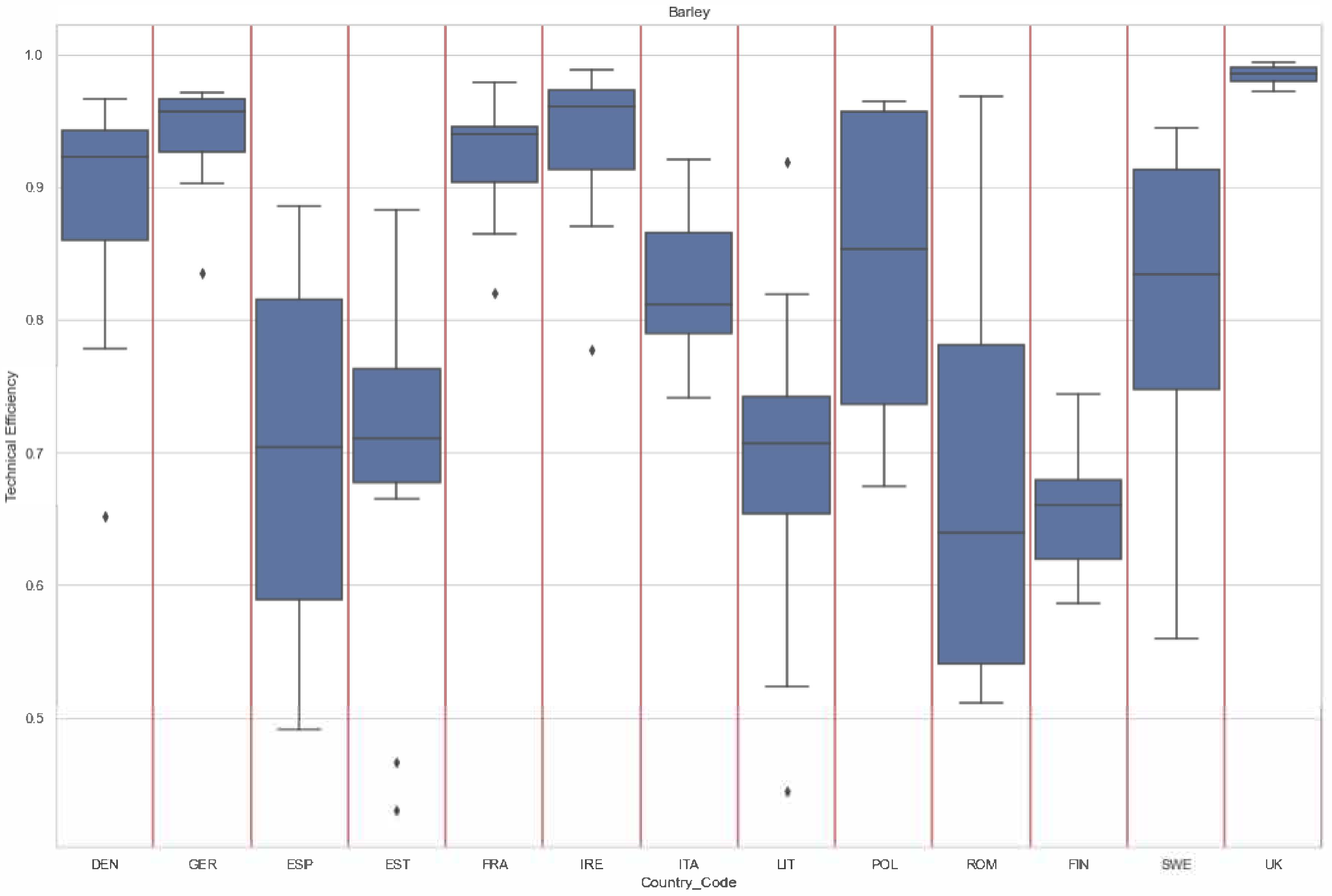
United Kingdom	0.985	0.007	0.972	0.994	0.985	0.008	0.971	0.994	-	-	-	-

presents the technical efficiency estimates distribution for barley, wheat, and maize across the countries considered in this study under the half-normal distribution. The highest efficiency level is in the United Kingdom, while Finland has the lowest technical efficiency. Specifically, the average level of technical efficiency estimates for the United Kingdom is 0.98, with a minimum of 0.97, a maximum of 0.99, and a standard deviation of 0.077. For Finland, the average is 0.65, with a minimum of 0.58, a maximum of 0.74, and a standard deviation of 0.050. It is surprising that other countries, such as Estonia, Lithuania, Romania, and Spain, have technical efficiencies lower than 0.70.

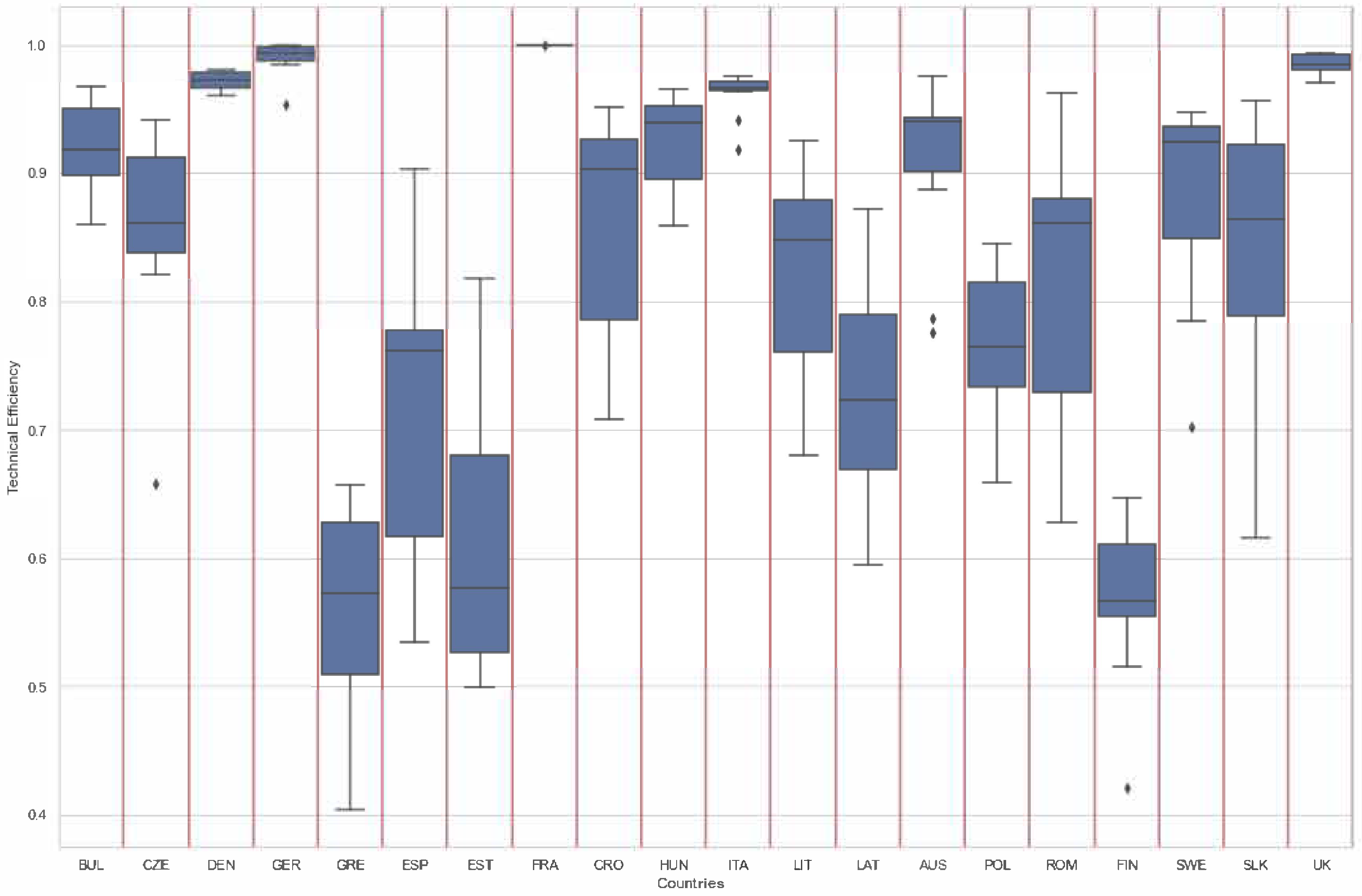
For wheat production, France has the highest technical efficiency, while Greece has the lowest. Using a half-normal distribution, France’s average level of technical efficiency is 0.993, with a minimum of 0.981 and a maximum of 1. Within the same distribution, however, the average for Greece is 0.56, with a range of 0.40–0.65 and a standard deviation of 0.086. The United Kingdom has an average efficiency of 0.985, with a minimum of 0.971, a maximum of 0.994, and a standard deviation of 0.008.

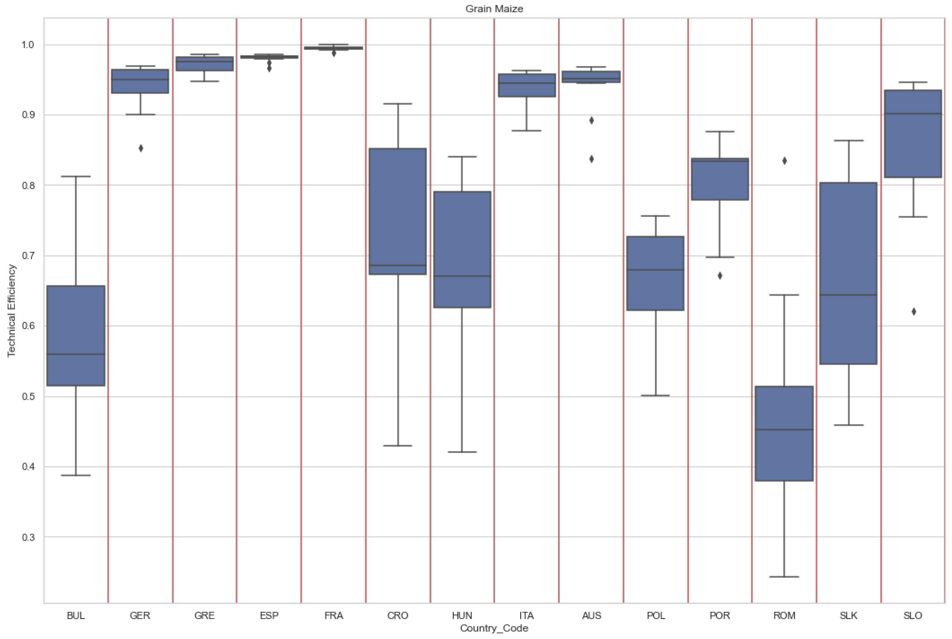
Regarding the grain maize, France has the highest technical efficiency, while Romania has the lowest. France’s average level of technical efficiency, using a half-normal distribution, is 0.994, with a minimum of 0.986 and a maximum of 1. The average for Romania is 0.48, ranging from 0.244 to 0.850. Bulgaria is another country with low technical efficiency in producing grain maize. Over the years, the TE averages 0.598, with a minimum of 0.397 and a maximum of 0.819. On the other hand, Poland and Slovakia’s maize productions exhibit a TE lower than 0.70.

However, the results provide a different story when examining the variation across the countries and years, as summarized in Figure 4, Figure 5 and Figure 6. The advantage of boxplots over summary statistics is that the former provide more information on the distribution and variability of the variable under consideration. For example, the boxplot provides information on the minimum, the maximum, the median, the first quartile, and the third quartile. It also provides information on the presence of outliers, the symmetry and skewness of the distribution, and whether the data are tightly grouped or not. Figure 4 gives the boxplot of barley’s technical efficiency score estimates under the half-normal distribution across the countries considered in the study. In the case of this study, the boxplot graph for each country provides the distribution of the technical efficiency score estimates over the years.

Examining the boxplot above, we notice a significant variability in the technical efficiency estimates. For example, the U.K. has the shortest boxplot, implying that there has not been a lot of variation in technical efficiency scores over the years. On the other hand, countries such as Poland, Romania, Spain, and Sweden have comparatively taller boxplots, indicating the higher variation of the technical efficiency estimates over the years. Another striking result is the inequality of the median values of the technical efficiency score estimates. Western European countries, such as the U.K., Germany, Ireland, and France, show high median values compared to Eastern European countries, such as Estonia, Lithuania, Romania, and Poland. The technical efficiency estimates are lower for Spain than other Western European countries, with scores as low as 0.491 compared to 0.972 in the U.K., 0.835 in Germany, or 0.820 in France.

Figure 5 provides the boxplot for technical efficiency for wheat across producing countries in Europe. We observe that countries such as the UK, Germany, France, and Italy show slight variations in technical efficiency scores over the years. In contrast, countries such as Spain, Greece, Estonia, Croatia, Lithuania, Latvia, Romania, and Slovakia exhibited high variability in technical efficiency scores over the years. It is also striking to observe that Spain and Greece, which have been part of the European Union since the 1980s, produce common wheat at a lower technical efficiency than countries such as Lithuania, Latvia, Croatia, and Romania, which recently joined the union.

Regarding the variability of the technical efficiency scores, Figure 6 displays their boxplots under the half-normal distribution. We notice that countries such as Germany, France, Spain, Austria, and Greece have their score values oscillating between 0.9 and 1 over the years, with a small amount of variance. In comparison, Romania’s technical efficiency scores vary considerably over the years between 0.24 and 0.65.

5. Conclusions

The objective of this study was to assess the technical efficiency scores for three crops—barley, wheat, and maize—across European countries. The research unfolds in three stages. Initially, a random forest algorithm is employed to pinpoint the most influential variables that account for variations in the production function and inefficiency levels. Subsequently, these identified variables are utilized to estimate the production function and technical efficiency scores under half-normal, exponential, and truncated normal distributions. Lastly, this study employed Vuong’s (1989) test to determine the model that best aligns with the available data.

For barley, the random forest estimation results indicate the most important variables explaining that the variation in production is the total utility area, the quantity of fertilizer, the quantity of seed, rent payment, crop protection, and machine and lubricants. For wheat, the total utility area is the most important variable, followed by the quantity of seed, crop protection, rent payment, the cost of the own capital, and the quantity of energy. For maize, the most important variables are the seed quantity, total area, expenditure on family labor, expenditure on contract work, rent payment, and the machine and lubricant quantity.

For the technical inefficiency results, the random forest findings indicate that, for barley, the most important variable affecting technical efficiency is agriculture value added as a percentage of GDP. For wheat, the unemployment rate as a percentage of the labor force is the most influential predictor of total technical efficiency. For maize, the most crucial variable in predicting the technical efficiency of grain maize is female employment in the industry.

When considering the average level of technical efficiency across all countries and years, the study shows that barley’s technical efficiency score ranges from 0.803 to 0.835, while wheat has a higher score of 0.855. However, maize has the lowest score, ranging from 0.716 to 0.774. The UK has the highest technical efficiency score for barley, while Finland has the lowest. France demonstrates the highest technical efficiency score for common wheat and grain maize, while Greece and Romania exhibit the lowest scores, respectively.

Various macroeconomic and subsidy variables affect the technical efficiency of barley production. Factors such as female wages, foreign direct investment, and total population have a positive effect, while forest area, other subsidies, and total unemployment rate have a negative effect. Other variables have no significant effect on technical efficiency in barley production. For wheat production, factors such as agricultural employment, wages, forest area, and total direct payments have a positive effect on technical efficiency, while factors such as urban population, unemployment rate, and subsidies have a negative effect. Decoupled payments have varying effects under different distributions. For maize production, factors such as employment in the industry and wages for males have a positive effect, while factors such as employment in the industry for females, wage for females, and agricultural land have a negative effect. Total support for rural development has a positive impact on the technical efficiency of grain maize production under the half-normal distribution.

In summary, the study unveils a variation in the technical efficiency scores across diverse crops and countries, revealing the complex nature of agricultural productivity. This disparity underscores the significance of considering unique challenges and opportunities inherent in the cultivation of different crops within specific national contexts. Furthermore, the impact of macroeconomic variables and agricultural policies on these efficiency scores becomes evident, highlighting the need for tailored strategies to optimize production capabilities and address sector-specific challenges across various nations. Such insights are pivotal for policymakers aiming to enhance the overall agricultural efficiency and sustainability on a global scale. However, it is essential to acknowledge that this study is not without limitations. The scope of our research does not encompass an exhaustive exploration of all potential influencing factors, and thus, some aspects may not have been fully addressed. While recognizing these shortcomings, the current study serves as a valuable foundation, and future research may delve deeper into specific unexplored dimensions for a more comprehensive understanding of technical efficiency in cereal production at the national level.

References

1. Kočišová, K. Application of the DEA on the measurement of efficiency in the EU countries. Agric. Econ. 2015, 61, 51–62. [Google Scholar] [CrossRef]
2. Kaur, M.; Mahal, A.K.; Sekhon, M.; Kingra, H. Technical efficiency of wheat production in Punjab: A Regional Analysis. Agric. Econ. Res. Rev. 2010, 23, 173–180. [Google Scholar]
3. Schils, R.; Olesen, J.E.; Kersebaum, K.C.; Rijk, B.; Oberforster, M.; Kalyada, V.; Khitrykau, M.; Gobin, A.; Kirchev, H.; Manolova, V.; et al. Cereal yield gaps across Europe. Eur. J. Agron. 2018, 101, 109–120. [Google Scholar] [CrossRef]
4. Nowak, A.; Kijek, T.; Domańska, K. Technical efficiency and its determinants in the European Union. Agric. Econ. 2015, 61, 275–283. [Google Scholar] [CrossRef]
5. Tzouvelekas, V.; Pantzios, C.J.; Fotopoulos, C. Empirical evidence of technical efficiency levels in Greek organic and conventional farms. Agric. Econ. Rev. 2002, 3, 49–60. [Google Scholar]
6. Tadesse, B.; Krishnamoorthy, S. Technical efficiency in paddy farms of Tamil Nadu: An analysis based on farm size and ecological zone. Agric. Econ. 1997, 16, 185–192. [Google Scholar] [CrossRef]
7. Vuong, Q.H. Likelihood ratio tests for model selection and non-nested hypotheses. Econom. J. Econom. Soc. 1989, 57, 307–333. [Google Scholar] [CrossRef]
8. Fried, H.O.; Lovell, C.K.; Schmidt, S.S. The Measurement of Productive Efficiency and Productivity Growth; Oxford University Press: Oxford, UK, 2008. [Google Scholar]
9. Cesaro, L.; Marongiu, S.; Arfini, F.; Donati, M.; Capelli, M.G. Methodology for Analysing Competitiveness, Efficiency and Economy of Scale: Use and Applications of DEA; FACEPA Deliverable; INEA: Latina, Italy, 2009; pp. 1–3. [Google Scholar]
10. Hueth, D.L. The Use of Subsidies to Achieve Efficient Resource Allocation in Upland Watersheds; Documento de Trabajo No. ENV-1 (marzo); Banco Interamericano de Desarrollo, División de Medio Ambiente: Washington, DC, USA, 1995. [Google Scholar]
11. Benedetti, I.; Branca, G.; Zucaro, R. Evaluating input use efficiency in agriculture through a stochastic frontier production: An application on a case study in Apulia (Italy). J. Clean. Prod. 2019, 236, 117609. [Google Scholar] [CrossRef]
12. Bravo-Ureta, B.E.; Evenson, R.E. Efficiency in agricultural production: The case of peasant farmers in eastern Paraguay. Agric. Econ. 1994, 10, 27–37. [Google Scholar] [CrossRef]
13. Seyoum, E.; Battese, G.E.; Fleming, E. Technical efficiency and productivity of maize producers in eastern Ethiopia: A study of farmers within and outside the Sasakawa-Global 2000 project. Agric. Econ. 1998, 19, 341–348. [Google Scholar]
14. Zhu, X.; Lansink, A.O. Impact of CAP subsidies on technical efficiency of crop farms in Germany, the Netherlands and Sweden. J. Agric. Econ. 2010, 61, 545–564. [Google Scholar] [CrossRef]
15. Chen, Z.; Huffman, W.E.; Rozelle, S. Farm technology and technical efficiency: Evidence from four regions in China. China Econ. Rev. 2009, 20, 153–161. [Google Scholar] [CrossRef]
16. Ghaderzadeh, H.; Rahimi, M.H. Estimation of technical efficiency of wheat farms: A case study in Kurdistan Province, Iran. Am.-Eurasian J. Agric. Environ. Sci. 2008, 4, 104–109. [Google Scholar]
17. Tzouvelekas, V.; Pantzios, C.J.; Fotopoulos, C. Economic efficiency in organic farming: Evidence from cotton farms in Viotia, Greece. J. Agric. Appl. Econ. 2001, 33, 35–48. [Google Scholar] [CrossRef]
18. Madau, F.A. Technical efficiency in organic and conventional farming: Evidence from Italian cereal farms. Agric. Econ. Rev. 2007, 8, 5–22. [Google Scholar]
19. Lansink, A.O.; Silva, E.; Stefanou, S. Inter-firm and intra-firm efficiency measures. J. Product. Anal. 2001, 15, 185–199. [Google Scholar] [CrossRef]
20. Latruffe, L.; Balcombe, K.; Davidova, S.; Zawalinska, K. Technical and scale efficiency of crop and livestock farms in Poland: Does specialization matter? Agric. Econ. 2005, 32, 281–296. [Google Scholar] [CrossRef]
21. Dimara, E.; Pantzios, C.J.; Skuras, D.; Tsekouras, K. The impacts of regulated notions of quality on farm efficiency: A DEA application. Eur. J. Oper. Res. 2005, 161, 416–431. [Google Scholar] [CrossRef]
22. Lambarraa, F.; Serra, T.; Gil, J. Technical efficiency analysis and decomposition of productivity growth of Spanish olive farms. Span. J. Agric. Res. 2007, 5, 259–270. [Google Scholar] [CrossRef]
23. Gadanakis, Y.; Bennett, R.; Park, J.; Areal, F.J. Improving productivity and water use efficiency: A case study of farms in England. Agric. Water Manag. 2015, 160, 22–32. [Google Scholar] [CrossRef]
24. Coelli, T.J.; Rao, D.S.P.; O’Donnell, C.J.; Battese, G.E. An Introduction to Efficiency and Productivity Analysis; Springer Science & Business Media: Berlin/Heidelberg, Germany, 2005. [Google Scholar]
25. Wang, T.; Cullinane, K.; Song, D.W. Container Port Production and Economic Efficiency; Springer: Berlin/Heidelberg, Germany, 2005. [Google Scholar]
26. Gebrie, A.; Mada, M. Technical Efficiency of Smallholder Wheat Producers in Simada District of Amhara Region, Ethiopia; College of Agriculture and Environmental Sciences, School of Graduate Studies: Gondar, Ethiopia, 2018. [Google Scholar]
27. Lovell, C.K. Production frontiers and productive efficiency. Meas. Product. Effic. Tech. Appl. 1993, 3, 67. [Google Scholar]
28. Aigner, D.J.; Chu, S.f. On estimating the industry production function. Am. Econ. Rev. 1968, 58, 826–839. [Google Scholar]
29. Aigner, D.; Lovell, C.K.; Schmidt, P. Formulation and estimation of stochastic frontier production function models. J. Econom. 1977, 6, 21–37. [Google Scholar] [CrossRef]
30. Meeusen, W.; van Den Broeck, J. Efficiency estimation from Cobb-Douglas production functions with composed error. Int. Econ. Rev. 1977, 18, 435–444. [Google Scholar] [CrossRef]
31. Battese, G.E.; Coelli, T.J. A model for technical inefficiency effects in a stochastic frontier production function for panel data. Empir. Econ. 1995, 20, 325–332. [Google Scholar] [CrossRef]
32. Kumbhakar, S.C.; Lovell, C.K. Stochastic Frontier Analysis; Cambridge University Press: Cambridge, UK, 2003. [Google Scholar]
33. Breiman, L. Random forests. Mach. Learn. 2001, 45, 5–32. [Google Scholar] [CrossRef]
34. Biau, G.; Scornet, E. A random forest guided tour. Test 2016, 25, 197–227. [Google Scholar] [CrossRef]
35. Greene, W.H. Econometric Analysis; Pearson Education India: Chennai, India, 2003. [Google Scholar]
Figure 1. Production frontiers and technical efficiency. Source: [24].
Sustainability 16 00546 g001
Figure 2. Productivity and efficiency. Source: [25].
Sustainability 16 00546 g002
Figure 3. The three-crop production distribution.
Sustainability 16 00546 g003
Figure 4. A boxplot for common barley under half-normal distribution across countries.
Sustainability 16 00546 g004
Figure 5. A boxplot for common wheat under half-normal distribution across countries.
Sustainability 16 00546 g005
Figure 6. A boxplot for grain maize under half-normal distribution across countries.
Sustainability 16 00546 g006