Article

Comparing the Evolution of Land Surface Temperature and Driving Factors between Three Different Urban Agglomerations in China

1
School of Civil Engineering and Geomatics, Shandong University of Technology, Zibo 255049, China
2
Key Laboratory of Urban Land Resources Monitoring and Simulation, Ministry of Natural Resources, Shenzhen 518040, China
3
School of Space Science and Physics, Shandong University, Weihai 264209, China
4
State Key Laboratory of Resource and Environmental Information System, Institute of Geographic Sciences and Natural Resources Research, Chinese Academy of Sciences, Beijing 100101, China
5
College of Earth Science, Chengdu University of Technology, Chengdu 610059, China
*
Author to whom correspondence should be addressed.
Sustainability 2024, 16(2), 486; https://doi.org/10.3390/su16020486
Submission received: 8 November 2023 / Revised: 27 December 2023 / Accepted: 27 December 2023 / Published: 5 January 2024

Abstract

:
Increases in land surface temperature (LST) and the urban heat island effect have become major challenges in the process of urban development. However, few studies have examined variations in LST between different urban agglomerations (UAs). Based on MODIS LST data, we quantitatively analyzed the spatial and temporal evolution patterns of LST in three different UAs in China from 2000 to 2020—Beijing–Tianjin–Hebei (BTH) at the national level, the Shandong Peninsula (SP) at the regional level, and Central Shanxi (CS) at the city level—by employing urban agglomeration built-up area intensity (UABI), linear regression analyses, and geodetic detector models. The results showed the following: (1) The spatial and temporal evolution pattern of the LST in BTH was the most regularized; the spatial pattern of the LST in SP gradually evolved from “two points” to “a single branch”; and the LST of CS was easily influenced by the neighboring big cities. (2) The best-fitting coefficients for BTH, SP, and CS were R2BTH = 0.58, R2SP = 0.66, and R2CS = 0.58, respectively; every 10% increase in UABI warmed the LSTs in BTH, SP, and CS by 1.47 °C, 1.27 °C, and 1.83 °C, respectively. (3) The ranking of single-factor influence was DEM (digital elevation model) > UABI > NDVI > T2m (air temperature at 2 m) > POP (population). The UABI interacting with DEM had the strongest warming effect on LST, with the maximum value q(UABI ∩ DEM) BTH = 0.951. All factor interactions showed an enhancement of the LST in CS, but factors interacting with POP showed a weaker effect in BTH and SP, for which q(NDVI ∩ POP) BTH = 0.265 and q(T2m ∩ POP) SP = 0.261. As the development of UAs gradually matures, the interaction with POP might have a cooling effect on the environment to a certain degree.

1. Introduction

In the 21st century, due to the combination of global warming, urban land expansion, and population growth, extreme heat events are occurring more frequently with non-negligible impacts on the survival and development of human beings [1,2]. Exposure to heat is expected to soar in the future, especially for cities in Africa and Asia [3], and high temperatures will intensify in urban areas, where temperatures may be a few degrees warmer than in surrounding areas; this is known as the urban heat island effect (UHI) [4,5]. The UHI effect is now widespread in industrial production and daily life, and it shows an increasing trend every year, causing a series of urban problems such as heat waves, air pollution, traffic congestion, and ecological damage [6].
Globally, UAs have become important factors for shifting the center of gravity of the world’s economy and will determine the future pattern of global economic development, making their status and roles more and more prominent [7]. The report of the 20th CPC National Congress systematically elaborated the connotation and essence of Chinese-style modernization and clearly put forward specific requirements such as “Striving to promote urban-rural integration and coordinated regional development” and “Constructing a coordinated development pattern of large, medium-sized and small cities relying on UAs and metropolitan circles”. UAs are dominant carriers of economic accumulation, industrialization, and urbanization. However, under the backdrop of economic growth in recent decades, serious environmental damage caused by urban heat is on the rise [8,9]. More research is needed to explore the mechanisms of urban heat impacts to prevent further environmental damage.
Regarding the diversity of methods used at the city level [10], many studies have used land surface temperature (LST) retrieval algorithms, spatial and temporal evolution characteristics, model analysis, linear regression analysis, and other approaches to explore the driving mechanisms of UHIs [11,12,13]. In these studies, the authors introduced various simulation methods (such as numerical simulation [14] and simulation models [15], regression fitting [16,17], and ecological landscape methods [18,19]). They also reported numerous conclusions, for example, that the UHI effect could be mitigated by replacing traditional roofs with cold roofs [20] and rationally allocating the appropriate geometry and diversity of blue and green spaces [21,22]. UAs have been studied using an equally rich array of research methodologies, leading to a variety of different conclusions. Fu et al. found that social and environmental factors were the main contributors to the variation in SUHII, which exhibited seasonal variation, based on dual metrics such as SUHI intensity and footprint [23]. Furthermore, Li et al. found that the NDVI in particular contributed to SUHI dynamics in all six factors studied [24]. From the perspective of resources and environmental carrying capacity (RECC), including urban heat, Fan et al. proved that advancements in industrial structures and an increase in residents’ consumption level were the main factors affecting the RECC of the SP UA [25]. Furthermore, an international study assessed seasonal variations in SUHI and discovered that SUHI was higher in core areas across UAs that were largely dominated by high-density residential zones [26]. In contrast, a New York study found that higher neighborhood NDVI and hyper-local tree, shrub, and grass cover decrease temperatures, whereas higher neighborhood building density increases temperature [27]. However, few studies have investigated the thermal environment in small- and medium-sized UAs, such as the regional-level SP UA and the city-level CS UA. Furthermore, there are almost no studies conducting comparative analyses among different UAs at different stages of development. Also, the spatial and temporal patterns of the LST across different Chinese UAs are still unclear, and the key driving mechanisms of nature and society have not been clarified. Therefore, there is a need to enrich relevant research by exploring the evolution patterns of LST among different classes of UAs in conjunction with emerging observational and modeling tools [28,29,30].
As a result, this study took three representative UAs of different levels in China (BTH, SP, and CS) as the research objects and compared the spatial and temporal variability in their LST patterns using MODIS LST data products, impervious surface data, and the intensity of the urban agglomeration built-up area (UABI). Finally, we quantitatively analyzed the driving mechanism of LST in UAs by combining the UABI, linear regression analysis, and Geo-detector models. The purpose of this study is to reveal the evolution characteristics of LST in UAs at different levels, compare their spatial and temporal differences, and investigate the driving mechanisms of LST. It is hoped that the results from our study could provide a scientific and theoretical basis for the mitigation of UAs’ UHI effect.

2. Materials and Methods

2.1. Study Area Overview

This study selected three major UAs in China according to Atlas of Chinese Cities published by C Fang in 2020, shown in Figure 1: the Beijing–Tianjin–Hebei national-level UA (BTH contains 13 cities, including 3 core cities: Beijing, Tianjin, and Shijiazhuang); the Shandong Peninsula regional-level UA (SP contains 16 cities, including 2 core cities: Jinan and Qingdao); and the Central Shanxi city-level UA (CS contains 8 cities, including only one core city: Taiyuan). BTH has the most mature urban agglomeration, with the highest degree of urbanization in China, SP has been urbanizing at an extremely fast pace since 2005, with a high level of development, and CS has emerged as a newly budding city cluster in recent years. The past two decades have seen rapid urbanization, which has caused significant changes in the factors affecting LST. Consequently, the effects of these factors on LST are now distinctly heterogeneous. Furthermore, these UAs have similar geographic environments and completely different numbers of core cities, making them ideal study areas for comparison.
(a) BTH: This is one of the five most maturely developed national-level UAs in China, located in the North China Plain, with a construction status area of approximately 183,400 km2. In 2022, the GDP of BTH was approximately 10 trillion RMB. The average temperature in summer (June, July, and August) was around 31.4 °C, and the average temperature in winter (December, January, and February) was around −2.1 °C [31]. (b) SP: This is one of the eight most rapidly developing regional-level UAs in China, located in the East China Plain, with a construction status area of approximately 113,100 km2. In 2022, the GDP of SP was approximately 8.3 trillion RMB. The average temperature in summer was around 28.2 °C, and in winter, around −2.6 °C [32]. (c) CS: This is one of the six emerging and most typical city-level UAs in China, located in the North China Plain, with an area of about 89,400 km2. In 2022, the GDP of CS was approximately 2 trillion RMB. The average temperature in summer was around 24.6 °C, and the average temperature in winter was around −4.3 °C.

2.2. Data Sources and Pre-Processing

The MOD11A2 data used in this study were collected from the Terra satellite with a spatial resolution of 1 km × 1 km, which is sufficient for the spatial characterization of LST at medium and large scales. For the UAs (BTH, SP, and CS), the spatial resolution and the observational frequency of twice every 8d are more suitable for mapping the evolution of LST. The monthly mean LST dataset was downloaded and computed through the synthesis of the MODLT1T product from the geospatial data cloud (https://www.gscloud.cn/) [33,34,35]. Since the dataset misses data for some months due to excessive cloudiness during 2000–2020, this study obtained supplementary MODIS 11A2 data from NASA to cover the whole study area and study period. Moreover, the 30 m precision impervious-surface dataset was used to calculate the normalized difference vegetation index (NDVI). Furthermore, population density and temperature were used for attribution analysis in Geo-detector models. Comprehensive information about the data used in this study is shown in Table 1.

2.3. Urban Agglomeration Built-Up Area Intensity (UABI)

The ratio of urban impervious surfaces to total regional land area was defined as urban intensity [36]. This was an important indicator to quantify the intensity of urban land development. In this study, we used the built-up area of the urban agglomeration as a percentage of total regional land area to characterize the UA built-up area intensity (UABI). The UABIs of BTH, SP, and CS were computed by generating 1 km × 1 km grids as the basic analysis unit. Based on the principle of spatial consistency, the constructed area grid scale was set to be consistent with the spatial resolution of MODIS LST product data by utilizing the Create fishnet tool provided by the ArcGIS 10.7 software platform. The Tabulate Area tool in ArcGIS was used to calculate the impervious surface area of each grid. In addition, in order to avoid the influence of water bodies on the relationships between UABI and LST, the dynamic dataset of impervious surfaces produced by L Liu’s team at the Chinese Academy of Sciences (CAS) was selected to exclude the water bodies and elevation in the study area, so as to guarantee the accuracy of the UABI. The formula for calculating the UABI is as follows:
U A B I i = B U A i G A i × 100 %
where U A B I i is the built-up area intensity of the urban agglomeration, B U A i denotes the built-up area in grid i , and G A i denotes the area of grid i 1 km × 1 km.

2.4. Land Surface Temperature Classification

To make the LST comparable in different study periods, the retrieved LST was modified to normalized LST (NLST) based on previous studies [37,38]. This was calculated by the following formula:
N L S T = T i T m i n T m a x T m i n
where NLST is the normalized LST value, T i is the original LST value of the image element, and T m a x and T m i n are the highest and lowest values of LST in the whole study area, respectively. Based on the range of NLST values, the standard deviation classification method was used to reclassify the NLST [39]. The NLST was further classified into seven different temperature regions with the support of ArcGIS 10.7 software, namely, lowest temperature, lower temperature, low temperature, medium temperature, high temperature, higher temperature, and highest temperature, as shown in Table 2 below.

2.5. Spatial Analysis and Statistical Regression Methods

The main spatial analysis method employed in this study was GIS, which was used to analyze the evolution characteristics of LST in UAs [40]. Statistical regression was carried out, including correlation analysis and linear regression analysis (LRA). Correlation analysis is a statistical method used to determine whether there is a correlation between variables and the strength of that correlation. The correlation coefficient is calculated to represent the strength of the correlation, with values ranging from −1 to 1. A value of 0 indicates no correlation between the variables, a value of 1 indicates a completely positive correlation, and a value of −1 indicates a completely negative correlation. The absolute value of the correlation coefficient indicates the strength of the correlation. LRA is used to determine the degree of the linear relationship between the independent and dependent variables by calculating the coefficient of determination (r2). The coefficient of determination (r2) takes a value in the range of (0,1], where a larger r2 indicates a higher degree of linear fit.
These methods were primarily used to investigate the impact of urban UABI on LST and to explore the mechanisms that influence LST [41].

2.6. Geo-Detector Model

Geo-detector 2015 software is a tool developed by Wang et al. [42,43] for detecting and exploiting spatial heterogeneity. It can be downloaded for free from the website (http://www.geodetector.cn/). Its core assumption is that if an independent variable has a significant effect on a dependent variable, then the spatial distributions of the independent and dependent variables should be similar [44]. Geo-detectors include factor detection, interaction detection, risk detection, and ecological detection. The method is based on the principle of dividing a region into smaller regions, which are heterogeneous if the sum of the variances of these smaller regions is less than the variance of the region. In addition, to spatially match the dependent variable Y and the independent variable X, Y is first spatially discretized uniformly (1 × 1 km grid cells) and then superimposed on the distribution of X. Y and X are extracted at each discretization point [45,46,47]. The formula is as follows:
q x = 1 h = 1 L N h σ h 2 N σ 2
where q x is the value of the indicator measuring the spatial association between X and Y; H = 1, 2, 3, …, L, where L is the number of strata (partitions or subclasses) of factor X; and N and N h are the number of samples in the study area and each stratum h, respectively. The symbols σ 2 and σ h 2 denote the variance in Y in the whole area and in each stratum (h), respectively. The value of q x ∈ [0, 1] indicates how much Y is affected by X, which means the larger the value of q x , the stronger the spatial association between X and Y [48,49].

3. Results

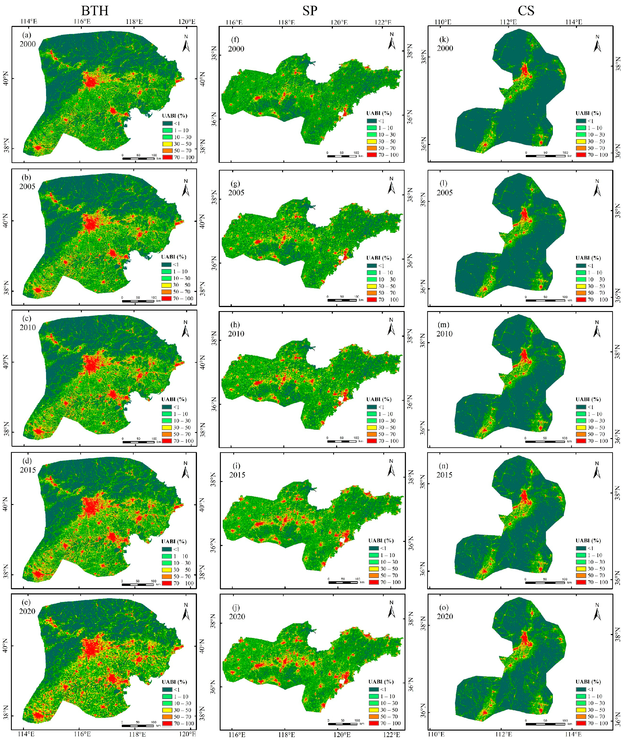
3.1. Spatial and Temporal Distribution of UABI in UAs of Different Levels

The spatial and temporal distributions of UABI for BTH, SP, and CS from 2000 to 2020 are shown in Figure 2. In terms of temporal evolution, the evolution pattern of UABI was similar in the three UAs: areas with low and medium UABI (<50%) were steadily increasing, and areas with UABI <10% represented the largest proportion in all of them. However, these three UAs also showed differences in UABI patterns, such as the number of urban cores and spatial patterns of low or medium UABI patches. BTH has three cores, Beijing, Tianjin, and Shijiazhuang, which were the cities with the most extensive and concentrated high UABI (>50%) patches in the region. In contrast, CS was supported by a single core, Taiyuan City, and had a high UABI share of less than 10%. SP, on the other hand, was driven by two cores, Qingdao and Jinan. It was clear that its core area had a lower “high UABI area” than BTH but was higher than that of CS. In addition, the areas of medium and high UABI (>30%) are clustered in the east–west direction of the line connecting the two cores.

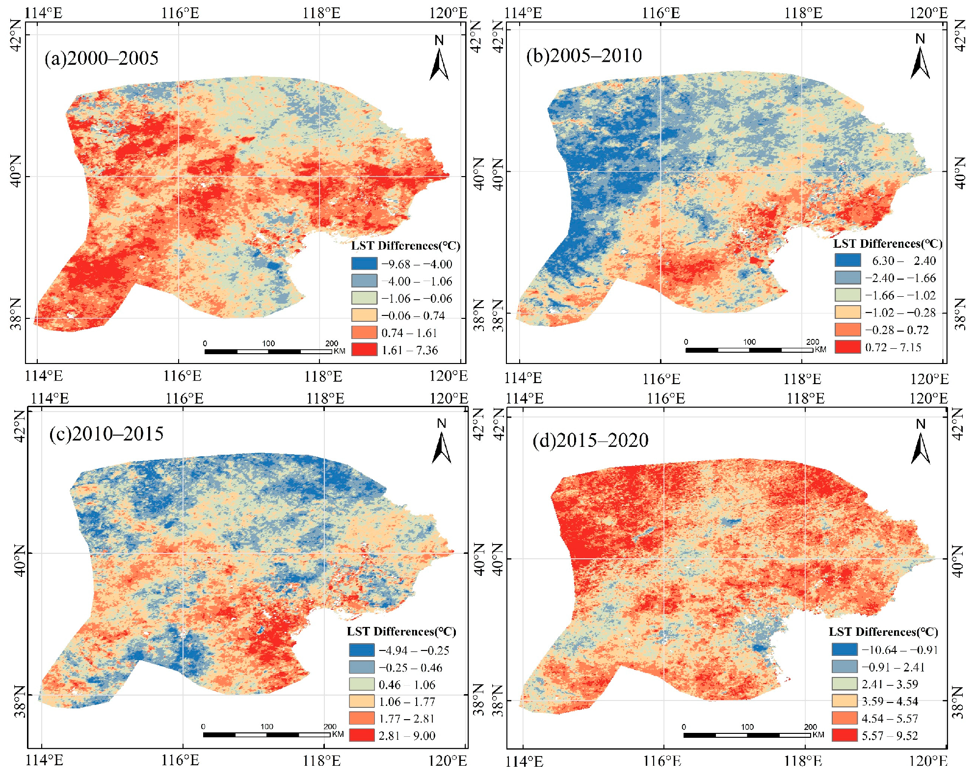
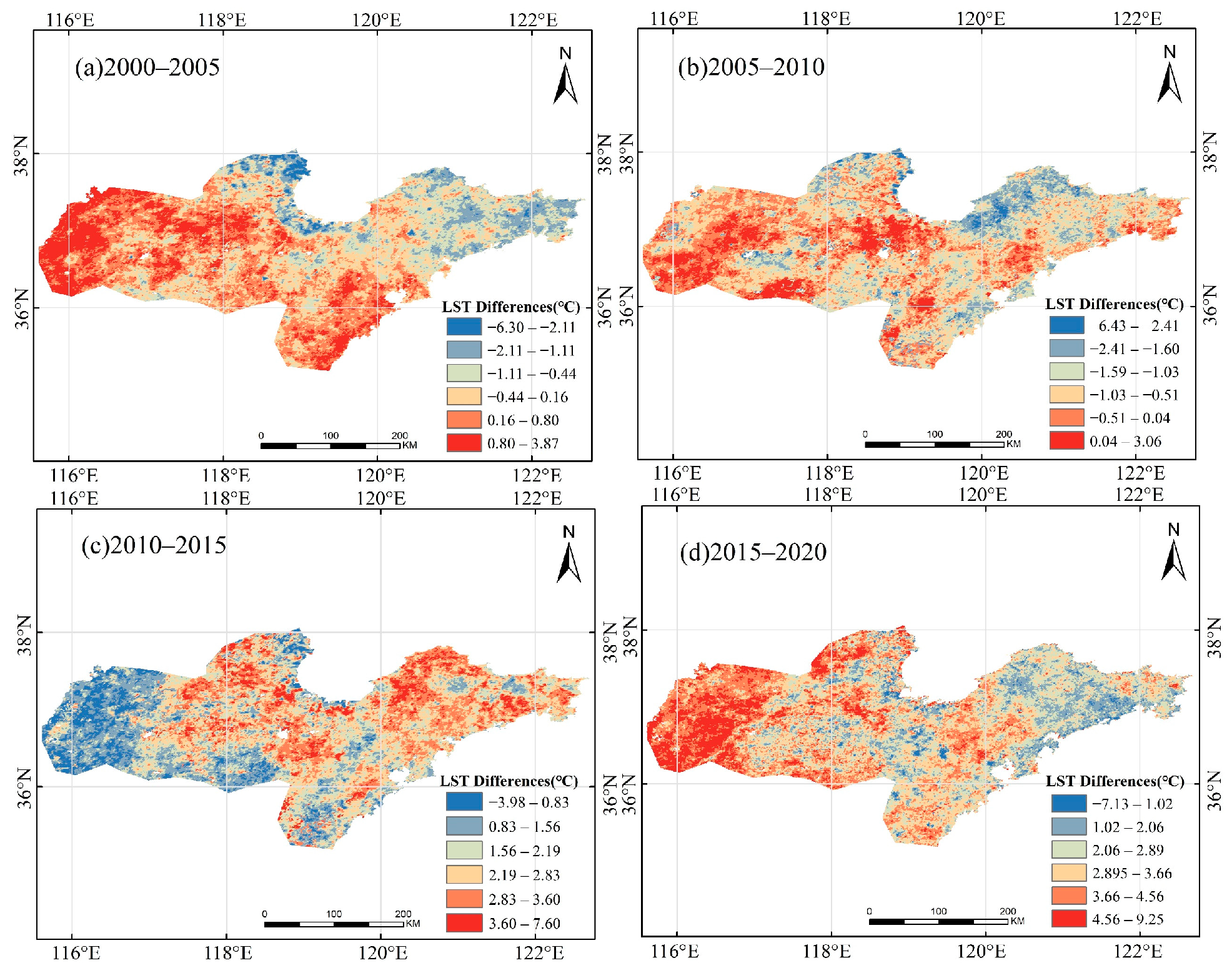
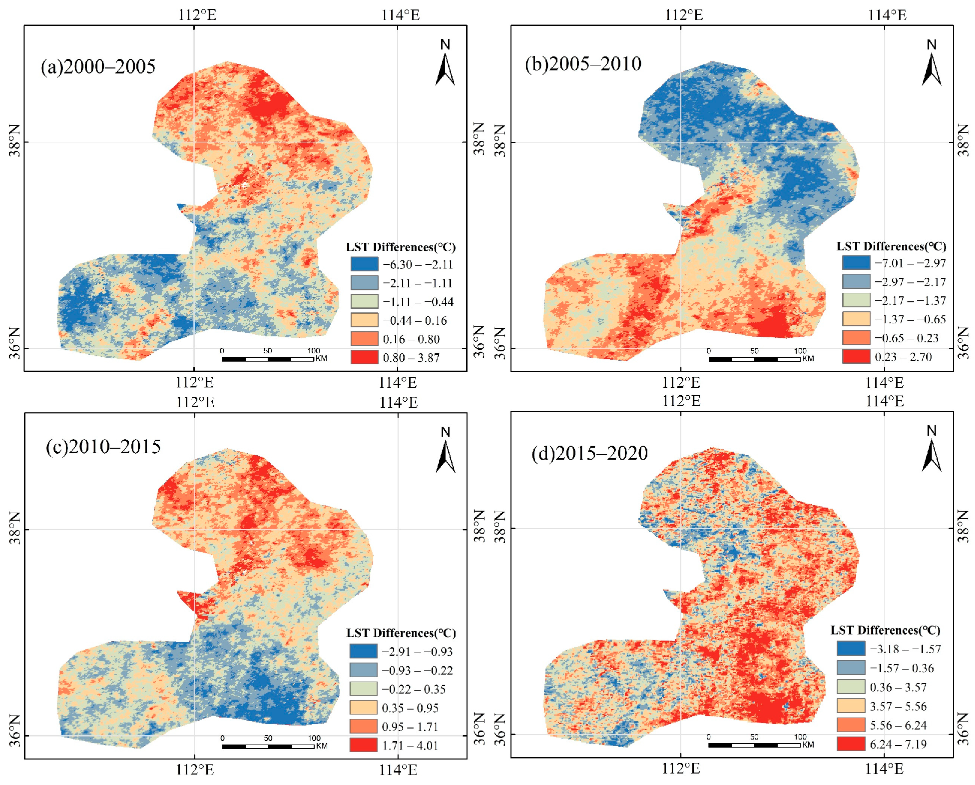
3.2. Characterization of the Spatial Evolution of LST in UAs of Different Levels

The spatial evolution of LST in BTH (Figure 3a–e), SP (Figure 3f–j), and CS (Figure 3k–o) is shown in Figure 3. The spatial pattern of LST in BTH from 2000 to 2020 varied in different stages. The high-temperature zone (including extremely high-temperature, high-temperature, and higher-temperature zones) was mainly concentrated in the centers of Beijing, Shijiazhuang, Tianjin, and other densely populated areas and their surroundings, as well as the border of Tianjin and Langfang. The low-temperature zone (including extremely low-temperature, low-temperature, and lower-temperature zones) has been gradually decreasing during the past 20 years. With more people moving into the BTH during these two decades, Beijing had the largest high-temperature zone, and the northern periphery of the BTH had a relatively low average temperature due to the high coverage of grasslands and forests. Figure 3f–j shows the spatial evolution of the LST in the CS region from 2000 to 2020, which indicates that the pattern of LST increased from a “point” to the “belt” connecting the two points of Jinan and Qingdao. Spatially, the distribution of LST changed from the line connecting Jinan and Qingdao to the north–south direction. The low-temperature zones were mainly concentrated in the coastal fringe areas of Dongying, Weifang, Weihai, and Yantai. However, Qingdao, as a coastal city, did not have any obvious low-temperature zones. High-temperature zones are distributed in the northeastern edge of the built-up area in CS, whereas low-temperature and medium-temperature zones are dispersed in large suburban areas between cities, as well as in mountainous plateaus and a small portion of the green areas.

3.3. Temporal Trends of LST in UAs of Different Levels

In this study, images showing differences in LST were obtained using the ArcGIS spatial analysis module to conduct a difference calculation of the LST from 2000 to 2020, as shown in Figure 4, Figure 5 and Figure 6. Positive numbers (warm colors) in the legend indicate that the LST was rising, and negative numbers (cold colors) indicate that the LST was falling. A larger absolute value indicates that the LST has a more obvious trend of warming or cooling. The transition colors indicate that the change in LST was not obvious.
Figure 4 shows that from 2000 to 2005, the LST in BTH changed significantly. The rising LST was mainly concentrated in the southwest and east of the built-up area. In Figure 4b, the built-up area showed a greater degree of cooling in the period of 2005–2010. As shown in Figure 4c, from 2010 to 2015, the warming trend in the port area centered on the southeastern part of Tianjin was more obvious than that of five years ago. With the continuous expansion of the built-up area to the surrounding area, it can be seen that there was a warming trend for LST in all directions. From 2015 to 2020, the built-up area in BTH still showed an obvious warming trend, and the most obvious warming area was in the northeast and northwest part.
The evolution of LST in SP from 2000 to 2005 is shown in Figure 5. The region with the most obvious rise in LST was mainly found in the southwest of the built-up area. The warming pattern continued until 2005–2010, when the two points in Jinan and Qingdao remained unchanged, but these points appeared to migrate to the center and northeast of Shandong Peninsula. In Figure 5c, for 2010–2015, the pattern of “two points into a surface” disappears, with the Jiaodong Peninsula region and the eastern part of Jinan City warming up significantly. From 2015 to 2020, “two points into a surface” evolves into “a single branch”, and a small cooling phenomenon was only observed in the northern part of Yantai City for the whole study area.
The evolution of LST in CS is shown in Figure 6. In 2000–2005, the capital of Shanxi Province, Taiyuan city, had a significant warming trend extending to its surrounding area, whereas in the south, there were only small warming patches. During 2005–2010, the spatial pattern of LST change was different from that in 2005–2010, with the warming areas mainly centered on the urban areas of Linfen and Chengzhi. There was a pattern of overall rapid warming in the built-up area of CS in 2015–2020, which was mainly centered on the urban areas of the cities and spread out in all directions.

3.4. Changing Trends in the Effect of UABI on LST in UAs of Different Levels

As can be seen from Figure 7a–e, the regression coefficient R2 between UABI and LST in BTH was the highest (0.58) in 2010, indicating that 58% of the warming effect on LST in 2010 can be explained by UABI. The LST rises by 1.47 °C for every 10% increase in the intensity of built-up areas, and the regression coefficients for other years are, respectively, R22000 = 0.46, R22005 = 0.50, R22015 = 0.55, and R22020 = 0.49. All the R2 values were greater than 0.45, indicating that the regression model could explain the variations in LST during these 20 years well. These results showed that the UABI had strong relationships with LST at all the different-sized UAs.

3.5. Results of the Driving Factors of Geo-detector in UAs of Different Levels

As shown in Figure 8, the q-value (0.867) of UABI was the largest in BTH, indicating that UABI had the most significant effect on LST in the UAs with the highest urbanization level. However, the q-value of UABI (0.588) was the smallest in SP, even smaller than CS (0.773), which showed that the positive impact of UABI on LST did not continue to increase as the levels of UAs increased.
Based on the strength of effect, the ranking of single influence factors in BTH was as follows: DEM (0.896) > UABI (0.867) > NDVI (0.537) > T2m (0.633) > POP (0.054); for SP: DEM (0.856) > UABI (0.588) >NDVI (0.514) > T2m (0.445) > POP (0.089); and CS: DEM (0.821) > UABI (0.773) > NDVI (0.389) > T2m (0.383) > POP (0.137). In these three UAs with different degrees of development, DEM has the most significant effect on LST, and its q-value was above 0.821 [50]. This result was due to the fact that the temperature decreases by 0.6 °C for every 100 m of altitude. The q-values of POP were the smallest (all less than 0.137), which indicates that the increase in population density in the UAs’ development process had a very weak effect on the LST (in which the q-value of POP in BTH was only 0.054). In addition, the effect of POP on LST was negatively correlated to the degree of development of the UAs. It is worth mentioning that the order of the influencing factors in the three UAs was identical: DEM > UABI > NDVI > T2m > POP. This means that the effects of these five influencing factors on the spatial distribution of LST in different environments are consistent.
Since the LST was affected by many factors, the explanatory ability of a single factor was usually limited. Therefore, it was necessary to further explore the interaction of different influencing factors. In this study, we applied the Geo-detector interaction detector to calculate the strength of the association between two influencing factors on the spatial distribution of LST, and the results are shown in Table 3, Table 4 and Table 5 below. Overall, the interaction between two different factors exhibits nonlinear enhancement {q(X1 ∩ X2) > [q(X1) + q(X2)]/2} and nonlinear weakening {q(X1 ∩ X2) < [q(X1) + q(X2)]/2} [51], where ∩ denotes the interaction between X1 and X2, suggesting that the interaction will further enhance or weaken the explanatory power of the influence factor on the LST effect.
As shown in Table 3, Table 4 and Table 5, it was found that all factors interacting with another could have an enhancing effect in CS. However, there are factors interacting with POP that produced an attenuating effect in both BTH and SP [q(NDVI ∩ POP) BTH = 0.265, q(T2m ∩ POP) SP = 0.261]. Overall, the interaction between UABI, NDVI, and DEM has the most significant warming effect on LST. The more mature the UA is, the more obvious the observed warming effect of UABI, and the interaction with POP (e.g., NDVI and T2m) has a certain cooling effect on the LST. The densely populated urban core typically has more greenery and man-made cooling measures, resulting in a localized cooling effect.

4. Discussion

4.1. Differences in Spatial Distribution Patterns of UABI

As can be seen from Figure 2, all three UAs are driven by their respective core cities. However, the specific spatial patterns of UABIs are significantly different: Primary UAs (budding) generally have only one core city (CS), and less than 10% of the area has high UABI patches. In primary UAs, the linkages between the core city and the neighboring cities are separated by a large area of low to medium UABI. When the UA develops to a certain level (mid-term), it may be driven by multi-core cities, e.g., SP has two cores. The SP has a significantly higher percentage of high and medium UABI patches than the CS. The high UABI in SP was clustered in the east–west direction along the connection line between the two cores. In contrast, BTH (mature) has three cores, with the largest share of high UABI patches. The medium and high UABIs are distributed in the southeast region of BTH with Beijing, Tianjin, and Shijiazhuang as the core cities.

4.2. Differences in Spatial Patterns of LST

In this study, the national-level urban agglomeration BTH (mature), the regional-level urban agglomeration SP (mid-term), and the city-level urban agglomeration CS (budding) were selected to study the temporal and spatial evolution of LST from 2000 to 2020. The results show that the evolution pattern of LST in the national-level UA BTH was relatively fixed. It is worth mentioning that during the 2008 Olympic Games, the LST in Beijing and its surroundings did not rise but fell, which may be related to the relocation of mining enterprises to the south in advance and the environmental protection policy, with the high-temperature area concentrated in the southwest corner of the built-up area and the low-temperature area gathered in the northeast.
For mid-term UAs like SP, it can be clearly seen that the spatial distribution of LST was different from that in BTH [52]. The high-temperature zones spread in all directions along the line connecting Jinan and Qingdao, whereas low-temperature zones clustered around the edges of the seaside cities. For UAs like CS, the LST was mainly centered in the built-up areas, and the dispersed high-temperature zones were separated from the low-temperature zones in the suburbs.

4.3. Differences in Temporal Evolution of LST

The temporal evolution of LST in the regional UA SP was mainly influenced by two points (Jinan and Qingdao), and the overall pattern of “two points become a surface” shows a gradual evolution to “one branch stands alone”. The influence of Jinan on the surrounding LST increased, and the influence of Qingdao decreased. The high-temperature zones in the built-up area were located around the border of Jinan and Qingdao, and the low-temperature area was mainly located at the edge of the seaside cities. The national-level UA BTH has the highest degree of urbanization, and its LST distribution shows a relatively fixed evolutionary pattern. The LST difference in CS had no obvious spatial pattern during the study period. In addition, the LST in CS was easily influenced by the neighboring maturely developed UAs or megacities.
The temporal variations in LST have similar changing trends in these three UAs. For example, the evolution of LST in BTH, SP, and CS shows a very obvious trend, where the high LST spread to the edges of the built-up areas. This trend was especially obvious in the period of 2015–2020. There were no obvious features that represented the evolution of LST in CS during the budding stage. The high-temperature zones are concentrated in the urban areas of each city, and these dispersed high-temperature zones are separated by the low-temperature zones in the suburbs and are easily affected by neighboring big cities [53].

4.4. Differences in Driving Mechanisms of LST

The driving mechanism of LST in these three UAs with different development levels was quantitatively analyzed using linear regression analysis and Geo-detector modeling. The results showed that the best-fit regression coefficient between the UABI and LST of BTH was R22010 = 0.58 (1.47 °C increase in LST for every 10% increase in UABI), the best-fit regression coefficient for SP was R22015 = 0.66 (1.27 °C increase in LST per 10% increase in UABI), and the best-fit regression coefficient for CS was R22020 = 0.55 (for every 10% increase in UABI, LST increased by 1.83 °C). The best-fit regression coefficient R2 of CS was the smallest (0.55), but its warming effect on LST was the largest (1.83 °C). The results of the single-factor test showed that the rank of the influencing factors in these three UAs was as follows: DEM > UABI > NDVI > T2m > POP.
For SP, Figure 7f–j show that the regression coefficient R2 of UABI and LST in 2015 was the highest (0.66), and the LST increased by 1.27 °C for every 10% increase in UABI. The smallest linear regression coefficient appeared in 2000 with an R2 of 0.34, and the warming effect of UABI on LST was not obvious in comparison with other years. A linear regression model of the UABI and LST of CS in 2000–2020 is shown in Figure 7k–o. The regression coefficient R2 of UABI and LST in 2020 was the highest (0.55), and the LST increased by 1.83 °C for every 10% increase in UABI; the smallest linear regression coefficient occurred in 2000, and the R2 was 0.40, which means that the warming effect of UABI on LST was not obvious compared with other years. It was noted that CS had the smallest R2 among the best-fit years, but its UABI had the most significant warming effect on LST (1.83 °C for every 10% increase in UABI). In 2005, the R2 of the three UAs was 0.50, and the warming effect of UABI on LST was the most pronounced in BTH (1.26 °C for every 10% increase in UABI), followed by CS (1.11 °C for every 10% increase in UABI), and SP was the least pronounced (0.92 °C for every 10% increase in UABI).
As shown in Table 3, in BTH, UABI ∩ DEM has the strongest enhancing effect (q = 0.951), followed by T2m ∩ DEM (q = 0.911), whereas NDVI ∩ POP has the most pronounced weakening effect (q = 0.265). This indicates that the joint influence of UABI and DEM had the greatest positive effect on the LST, and the interaction of T2m and DEM also had an obvious warming effect, whereas the interaction between NDVI and POP (q = 0.265) had a certain cooling effect. In Table 4, the most obvious enhancement effect of SP on LST was the interaction between NDVI and DEM (q = 0.934), followed by the interaction between UABI ∩ DEM (q = 0.905), and the most obvious weakening effect was the interaction between T2m ∩ POP (q = 0.261). However, all the interactions between factors in CS showed enhancement (Table 5), with NDVI ∩ DEM having the most significant warming effect (q = 0.896). The warming effect of the interconnection of UABI and DEM (q = 0.871) closely followed, and UABI ∩ POP (q = 0.453) had the smallest effect on the warming of LST.
In the three UAs with different levels of development, the interaction of UABI, NDVI, and DEM had the most significant warming effect on LST. However, the warming effect of UABI on LST was even negligible under the interaction of UABI with POP in the UAs with a lower urbanization level (CS). In CS, the interaction of all the factors shows an enhancing effect, whereas in BTH and SP, there are factors that weaken the interaction with POP [q (NDVI ∩ POP) BTH = 0.265, q (T2m ∩ POP) SP = 0.261].

4.5. Differences and Similarities of Thermal Environments in UAs of Different Levels

Urban heat is a common challenge for many cities worldwide, and it is becoming intense, frequent, and severe [54,55]. In this paper, UABI was used to distinguish the three different levels of UAs, and the thermal environments of these UAs were comparatively analyzed in terms of both the spatial and temporal differences in LSTs and the mechanisms of influence. We found that the more mature UAs have more regular and fixed spatial and temporal distributions of LST and UABI. Despite the obvious differences in these spatial and temporal distributions, there is some similarity in the mechanism of influence on LST. The order of the contribution of individual factors to LST was exactly the same: UABI was the factor that best fits LST and has the most pronounced warming effect apart from DEM. However, in terms of the deeper influence mechanism, the interaction between factors, and the combined analysis, all factors except POP have more pronounced warming effects in the more mature UAs. Beyond the BTH, SP, and CS regions, this study can further generate imperative implications for the development of heat action plans (e.g., preparation, mitigation, and adaptation) for international cities that are experiencing urban heat challenges.

5. Conclusions

The linear regression analysis combined with Geo-detector modeling provided an opportunity to explore the influence mechanism of LST and its variability among UAs of different levels. From this study, we drew the following conclusions:
  • UAs of different levels showed a gradual evolution of LST. There was a positive correlation between the proportion of high-LST areas and the number of core cities. Urban heat islands (UHIs) were mainly concentrated in and around core cities.
  • UABI was the indicator factor that had the strongest effect on LST following DEM in the three UAs. Particularly in the city-level UAs, the LST increased by 1.83 °C for every 10% increase in UABI.
  • In national-level and regional-level UAs, the interactions of some factors with POP showed certain cooling effects on LST. In contrast, in the city-level UA, all factors and their interactions enhanced LST, albeit with varying intensities.
This study’s findings may aid planners and policymakers in identifying the variations in thermal environments and mechanisms of LST changes in UAs of different levels. This, in turn, can help integrate sustainability and proposed land use planning for better urban climate management. In future studies, the addition of more indicator factors must be considered to explore the deeper mechanisms influencing LST. The three different levels of UAs analyzed in the study area in this paper can be expanded to consider the different levels of UAs in the whole of China, or even the whole world, which are the areas that need to be investigated in subsequent work.

Author Contributions

Methodology, A.J. and T.K.; investigation, J.H.; writing—original draft preparation, L.P.; writing—review and editing, C.Y.; supervision, F.Y. All authors have read and agreed to the published version of the manuscript.

Funding

This study was funded by the National Natural Science Foundation of China (grant number 42201123) and the China Postdoctoral Science Foundation (grant number 2022M713309). This study was also supported by the Open Fund of the Key Laboratory of Urban Land Resources Monitoring and Simulation (KF-2022-07-002), Ministry of Natural Resources.

Institutional Review Board Statement

Not applicable.

Data Availability Statement

The data presented in this study are available on request from the corresponding author.

Conflicts of Interest

The authors declare no conflict of interest.

References

  1. Massaro, E.; Schifanella, R.; Piccardo, M.; Caporaso, L.; Taubenböck, H.; Cescatti, A.; Duveiller, G. Spatially-optimized urban greening for reduction of population exposure to land surface temperature extremes. Nat. Commun. 2023, 14, 2903. [Google Scholar] [CrossRef] [PubMed]
  2. Osborn, T.J.; Jones, P.D.; Lister, D.H.; Morice, C.P.; Simpson, I.R.; Winn, J.; Hogan, E.; Harris, I.C. Land surface air temperature variations across the globe updated to 2019: The CRUTEM5 data set. J. Geophys. Res. Atmos. 2021, 126, e2019JD032352. [Google Scholar] [CrossRef]
  3. Cai, D.; Fraedrich, K.; Guan, Y.; Guo, S.; Zhang, C.; Sun, R.; Wu, Z. Remote Sensing Greenness and Urbanization in Ecohydrological Model Analysis: Asia and Australasia (1982–2015). Sensors 2019, 19, 4693. [Google Scholar] [CrossRef] [PubMed]
  4. Oke, T.R. The energetic basis of the urban heat island. Q. J. R. Meteorol. Soc. 1982, 108, 1–24. [Google Scholar] [CrossRef]
  5. Cai, D.; Fraedrich, K.; Guan, Y.; Guo, S.; Zhang, C.; Zhu, X. Urbanization and climate change: Insights from eco-hydrological diagnostics. Sci. Total Environ. 2019, 647, 29–36. [Google Scholar] [CrossRef] [PubMed]
  6. Huang, K.; Li, X.; Liu, X.; Seto, K.C. Projecting global urban land expansion and heat island intensification through 2050. Environ. Res. Lett. 2019, 14, 114037. [Google Scholar] [CrossRef]
  7. Fang, C.; Yu, D. Urban agglomeration: An evolving concept of an emerging phenomenon. Landsc. Urban Plan. 2017, 162, 126–136. [Google Scholar] [CrossRef]
  8. Dadashpoor, H.; Azizi, P.; Moghadasi, M. Land use change, urbanization, and change in landscape pattern in a metropolitan area. Sci. Total Environ. 2019, 655, 707–719. [Google Scholar] [CrossRef]
  9. Fang, C.; Liu, H.; Wang, S. The coupling curve between urbanization and the eco-environment: China’s urban agglomeration as a case study. Ecol. Indic. 2021, 130, 108107. [Google Scholar] [CrossRef]
  10. Liu, H.; He, B.-J.; Gao, S.; Zhan, Q.; Yang, C. Influence of non-urban reference delineation on trend estimate of surface urban heat island intensity: A comparison of seven methods. Remote Sens. Environ. 2023, 296, 113735. [Google Scholar] [CrossRef]
  11. Jiménez-Muñoz, J.C.; Sobrino, J.A.; Skoković, D.; Mattar, C.; Cristobal, J. Land surface temperature retrieval methods from Landsat-8 thermal infrared sensor data. IEEE Geosci. Remote Sens. Lett. 2014, 11, 1840–1843. [Google Scholar] [CrossRef]
  12. Li, Y.; Zhou, D.-C.; Yan, Z.-M. Spatiotemporal variations in atmospheric urban heat island effects and their driving factors in 84 major Chinese cities. Huan Jing Ke Xue Huanjing Kexue 2021, 42, 5037–5045. [Google Scholar] [PubMed]
  13. Li, Y.; Wang, L.; Liu, M.; Zhao, G.; He, T.; Mao, Q. Associated determinants of surface urban heat islands across 1449 cities in China. Adv. Meteorol. 2019, 2019, 4892714. [Google Scholar] [CrossRef]
  14. Zheng, Y.; Liu, S.; He, P.; Miao, Y.; Wang, S. Numerical Study of Summertime Urban Heat Island in Dianzhong. Beijing Da Xue Xue Bao 2017, 53, 639–651. [Google Scholar]
  15. Schwarz, N.; Manceur, A.M. Analyzing the influence of urban forms on surface urban heat islands in Europe. J. Urban Plan. Dev. 2015, 141, A4014003. [Google Scholar] [CrossRef]
  16. Yang, C.; Yan, F.; Lei, X.; Ding, X.; Zheng, Y.; Liu, L.; Zhang, S. Investigating seasonal effects of dominant driving factors on urban land surface temperature in a snow-climate city in China. Remote Sens. 2020, 12, 3006. [Google Scholar] [CrossRef]
  17. Adulkongkaew, T.; Satapanajaru, T.; Charoenhirunyingyos, S.; Singhirunnusorn, W. Effect of land cover composition and building configuration on land surface temperature in an urban-sprawl city, case study in Bangkok Metropolitan Area, Thailand. Heliyon 2020, 6, e04485. [Google Scholar] [CrossRef]
  18. Zhao, H.; Tan, J.; Ren, Z.; Wang, Z. Spatiotemporal characteristics of urban surface temperature and its relationship with landscape metrics and vegetation cover in rapid urbanization region. Complexity 2020, 2020, 7892362. [Google Scholar] [CrossRef]
  19. Jay, O.; Capon, A.; Berry, P.; Broderick, C.; de Dear, R.; Havenith, G.; Honda, Y.; Kovats, R.S.; Ma, W.; Malik, A. Reducing the health effects of hot weather and heat extremes: From personal cooling strategies to green cities. Lancet 2021, 398, 709–724. [Google Scholar] [CrossRef]
  20. Imran, H.M.; Kala, J.; Ng, A.; Muthukumaran, S. Effectiveness of green and cool roofs in mitigating urban heat island effects during a heatwave event in the city of Melbourne in southeast Australia. J. Clean. Prod. 2018, 197, 393–405. [Google Scholar] [CrossRef]
  21. Dugord, P.-A.; Lauf, S.; Schuster, C.; Kleinschmit, B. Land use patterns, temperature distribution, and potential heat stress risk–the case study Berlin, Germany. Computers. Environ. Urban Syst. 2014, 48, 86–98. [Google Scholar] [CrossRef]
  22. Gunawardena, K.R.; Wells, M.J.; Kershaw, T. Utilising green and bluespace to mitigate urban heat island intensity. Sci. Total Environ. 2017, 584, 1040–1055. [Google Scholar] [CrossRef] [PubMed]
  23. Fu, X.; Yao, L.; Xu, W.; Wang, Y.; Sun, S. Exploring the multitemporal surface urban heat island effect and its driving relation in the Beijing-Tianjin-Hebei urban agglomeration. Appl. Geogr. 2022, 144, 102714. [Google Scholar] [CrossRef]
  24. Li, K.; Chen, Y.; Wang, M.; Gong, A. Spatial-temporal variations of surface urban heat island intensity induced by different definitions of rural extents in China. Sci. Total Environ. 2019, 669, 229–247. [Google Scholar] [CrossRef] [PubMed]
  25. Fan, W.; Song, X.; Liu, M.; Shan, B.; Ma, M.; Liu, Y. Spatio-temporal evolution of resources and environmental carrying capacity and its influencing factors: A case study of Shandong Peninsula urban agglomeration. Environ. Res. 2023, 234, 116469. [Google Scholar] [CrossRef] [PubMed]
  26. Saha, S.; Saha, A.; Das, M.; Saha, A.; Sarkar, R.; Das, A. Analyzing spatial relationship between land use/land cover (LULC) and land surface temperature (LST) of three urban agglomerations (UAs) of Eastern India. Remote Sens. Appl. Soc. Environ. 2021, 22, 100507. [Google Scholar] [CrossRef]
  27. Johnson, S.; Ross, Z.; Kheirbek, I.; Ito, K. Characterization of intra-urban spatial variation in observed summer ambient temperature from the New York City Community Air Survey. Urban Clim. 2020, 31, 100583. [Google Scholar] [CrossRef]
  28. Barlow, J.; Best, M.; Bohnenstengel, S.I.; Clark, P.; Grimmond, S.; Lean, H.; Christen, A.; Emeis, S.; Haeffelin, M.; Harman, I.N. Developing a research strategy to better understand, observe, and simulate urban atmospheric processes at kilometer to subkilometer scales. Bull. Am. Meteorol. Soc. 2017, 98, ES261–ES264. [Google Scholar] [CrossRef]
  29. Best, M.J.; Grimmond, C.S.B. Key conclusions of the first international urban land surface model comparison project. Bull. Am. Meteorol. Soc. 2015, 96, 805–819. [Google Scholar] [CrossRef]
  30. Bohnenstengel, S.; Belcher, S.; Aiken, A.; Allan, J.; Allen, G.; Bacak, A.; Bannan, T.; Barlow, J.; Beddows, D.C.; Bloss, W. Meteorology, air quality, and health in London: The ClearfLo project. Bull. Am. Meteorol. Soc. 2015, 96, 779–804. [Google Scholar] [CrossRef]
  31. Liu, L.; Lei, Y.; Zhuang, M.; Ding, S. The impact of climate change on urban resilience in the Beijing-Tianjin-Hebei region. Sci. Total Environ. 2022, 827, 154157. [Google Scholar] [CrossRef] [PubMed]
  32. Zhai, F.; Liu, Z.; Li, P.; Gu, Y.; Hu, L.; Sun, L.; Yang, B. Monthly and Interannual Variations in Winter Positive Surface-Bottom Temperature Difference in Northeastern Coastal Waters of the Shandong Peninsula in the Yellow Sea. J. Geophys. Res. Ocean. 2021, 126, e2021JC017562. [Google Scholar] [CrossRef]
  33. Freitas, S.C.; Trigo, I.F.; Bioucas-Dias, J.M.; Gottsche, F.-M. Quantifying the uncertainty of land surface temperature retrievals from SEVIRI/Meteosat. IEEE Trans. Geosci. Remote Sens. 2009, 48, 523–534. [Google Scholar] [CrossRef]
  34. Freitas, S.C.; Trigo, I.F.; Macedo, J.; Barroso, C.; Silva, R.; Perdigão, R. Land surface temperature from multiple geostationary satellites. Int. J. Remote Sens. 2013, 34, 3051–3068. [Google Scholar] [CrossRef]
  35. Trigo, I.F.; Monteiro, I.T.; Olesen, F.; Kabsch, E. An assessment of remotely sensed land surface temperature. J. Geophys. Res. Atmos. 2008, 113, 1–12. [Google Scholar] [CrossRef]
  36. Jia, W.; Zhao, S. Trends and drivers of land surface temperature along the urban-rural gradients in the largest urban agglomeration of China. Sci. Total Environ. 2020, 711, 134579. [Google Scholar] [CrossRef] [PubMed]
  37. Cui, Y.; Xu, X.; Dong, J.; Qin, Y. Influence of urbanization factors on surface urban heat island intensity: A comparison of countries at different developmental phases. Sustainability 2016, 8, 706. [Google Scholar] [CrossRef]
  38. Cruz, J.; Blanco, A.; Garcia, J.; Santos, J.; Moscoso, A. Evaluation of the cooling effect of green and blue spaces on urban microclimate through numerical simulation: A case study of Iloilo River Esplanade, Philippines. Sustain. Cities Soc. 2021, 74, 103184. [Google Scholar] [CrossRef]
  39. Yang, C.; Zhu, W.; Sun, J.; Xu, X.; Wang, R.; Lu, Y.; Zhang, S.; Zhou, W. Assessing the effects of 2D/3D urban morphology on the 3D urban thermal environment by using multi-source remote sensing data and UAV measurements: A case study of the snow-climate city of Changchun, China. J. Clean. Prod. 2021, 321, 128956. [Google Scholar] [CrossRef]
  40. Yang, C.; Yan, F.; Zhang, S. Comparison of land surface and air temperatures for quantifying summer and winter urban heat island in a snow climate city. J. Environ. Manag. 2020, 265, 110563. [Google Scholar] [CrossRef]
  41. Shen, Z.; Xu, X.; Xu, S.; Sun, D. A comparative study of land development patterns and regional thermal environments (RTEs) in typical urban agglomerations of China and America: A case study of Beijing-Tianjin-Hebei (BTH) and Boswash. Sci. Total Environ. 2022, 803, 149735. [Google Scholar] [CrossRef] [PubMed]
  42. Wang, J.F.; Li, X.H.; Christakos, G.; Liao, Y.L.; Zhang, T.; Gu, X.; Zheng, X.Y. Geographical detectors-based health risk assessment and its application in the neural tube defects study of the Heshun Region, China. Int. J. Geogr. Inf. Sci. 2010, 24, 107–127. [Google Scholar] [CrossRef]
  43. Wang, J.-F.; Zhang, T.-L.; Fu, B.-J. A measure of spatial stratified heterogeneity. Ecol. Indic. 2016, 67, 250–256. [Google Scholar] [CrossRef]
  44. Zhao, R.; Zhan, L.; Yao, M.; Yang, L. A geographically weighted regression model augmented by Geodetector analysis and principal component analysis for the spatial distribution of PM2.5. Sustain. Cities Soc. 2020, 56, 102106. [Google Scholar] [CrossRef]
  45. Wang, H.; Qin, F.; Xu, C.; Li, B.; Guo, L.; Wang, Z. Evaluating the suitability of urban development land with a Geodetector. Ecol. Indic. 2021, 123, 107339. [Google Scholar] [CrossRef]
  46. Wang, Y.; Wang, X.; Chen, W.; Qiu, L.; Wang, B.; Niu, W. Exploring the path of inter-provincial industrial transfer and carbon transfer in China via combination of multi-regional input–output and geographically weighted regression model. Ecol. Indic. 2021, 125, 107547. [Google Scholar] [CrossRef]
  47. Wang, Y.; Wen, H.; Sun, D.; Li, Y. Quantitative assessment of landslide risk based on susceptibility mapping using random forest and geodetector. Remote Sens. 2021, 13, 2625. [Google Scholar] [CrossRef]
  48. Tao, H.; Liao, X.; Li, Y.; Xu, C.; Zhu, G.; Cassidy, D.P. Quantifying influences of interacting anthropogenic-natural factors on trace element accumulation and pollution risk in karst soil. Sci. Total Environ. 2020, 721, 137770. [Google Scholar] [CrossRef]
  49. Huang, S.; Yu, L.; Cai, D.; Zhu, J.; Liu, Z.; Zhang, Z.; Nie, Y.; Fraedrich, K. Driving mechanisms of urbanization: Evidence from geographical, climatic, social-economic and nighttime light data. Ecol. Indic. 2023, 148, 110046. [Google Scholar] [CrossRef]
  50. Good, E.J.; Ghent, D.J.; Bulgin, C.E.; Remedios, J.J. A spatiotemporal analysis of the relationship between near-surface air temperature and satellite land surface temperatures using 17 years of data from the ATSR series. J. Geophys. Res. Atmos. 2017, 122, 9185–9210. [Google Scholar] [CrossRef]
  51. Chen, Y.; Zhou, Y.; Zhang, H.; Wang, C.; Wang, X. Spatiotemporal variations of surface ozone and its influencing factors across Tibet: A Geodetector-based study. Sci. Total Environ. 2022, 813, 152651. [Google Scholar] [CrossRef] [PubMed]
  52. Yang, C.; He, X.; Yan, F.; Yu, L.; Bu, K.; Yang, J.; Chang, L.; Zhang, S. Mapping the influence of land use/land cover changes on the urban heat island effect—A case study of Changchun, China. Sustainability 2017, 9, 312. [Google Scholar] [CrossRef]
  53. Feng, Z.; Wang, X.; Yuan, J.; Zhang, Y.; Yu, M. Changes in air pollution, land surface temperature, and urban heat islands during the COVID-19 lockdown in three Chinese urban agglomerations. Sci. Total Environ. 2023, 892, 164496. [Google Scholar] [CrossRef] [PubMed]
  54. Cai, D.; Fraedrich, K.; Guan, Y.; Guo, S.; Zhang, C. Urbanization and the thermal environment of Chinese and US-American cities. Sci. Total Environ. 2017, 589, 200–211. [Google Scholar] [CrossRef]
  55. He, B.-J. Cause-related injustice, process-related injustice, effect-related injustice and regional heat action planning priorities: An empirical study in Yangtze River Delta and Chengdu-Chongqing urban agglomerations. Landsc. Urban Plan. 2023, 237, 104800. [Google Scholar] [CrossRef]
Figure 1. Overview map of the study areas: (a) Beijing–Tianjin–Hebei national-level UA (BTH). (b) Shandong Peninsula regional-level UA (SP). (c) Central Shanxi city-level UA (CS).
Sustainability 16 00486 g001
Figure 2. Spatial distribution of UABI in BTH, SP, and CS from 2000 to 2020 (the areas with UABI <1% are mountains, rivers, water, etc.). Characterization of the spatial and temporal evolution of LST in UAs. BTH: (ae); SP: (fj); CS: (ko).
Sustainability 16 00486 g002
Figure 3. Spatial and temporal evolution of LST in 3 UAs (BTH, SP, and CS), 2000–2020: BTH: (ae); SP: (fj); CS: (ko).
Sustainability 16 00486 g003
Figure 4. LST difference map of BTH urban agglomeration: (a) Difference in LST in BTH from 2000 to 2005. (b) Difference in LST in BTH from 2005 to 2010. (c) Difference in LST in BTH from 2010 to 2015. (d) Difference in LST in BTH from 2015 to 2020.
Sustainability 16 00486 g004
Figure 5. LST difference map of SP urban agglomeration: (a) Difference in LST in SP from 2000 to 2005. (b) Difference in LST in SP from 2005 to 2010. (c) Difference in LST in SP from 2010 to 2015. (d) Difference in LST in SP from 2015 to 2020.
Sustainability 16 00486 g005
Figure 6. LST difference map of CS urban agglomeration: (a) Difference in LST in CS from 2000 to 2005. (b) Difference in LST in CS from 2005 to 2010. (c) Difference in LST in CS from 2010 to 2015. (d) Difference in LST in CS from 2015 to 2020.
Sustainability 16 00486 g006
Figure 7. The regression model built for UABI and LST in three UAs (BTH, SP, and CS) from 2000 to 2020: BTH: (ae); SP: (fj); CS: (ko).
Sustainability 16 00486 g007
Figure 8. Nonlinear effects of q-values of individual factors on the spatial distribution of LST in the UAs.
Sustainability 16 00486 g008
Table 1. Data sources and description.
DataData DescriptionData SourcesData Use
Scope of the UAsScope of the current status of urban agglomeration constructionAtlas of Chinese CitiesUA built-up area identification
Land cover30 m nationwide annual land cover dataZenodo Data Download CenterCharting
Land surface temperature1 km monthly mean LST data product, MODIS 11A2Geospatial Data Cloud and NASADynamic analysis
Impervious surface30 m impervious-surface dynamic datasetZenodo Data Download Center Produced by L Liu Team, CASCalculation of U A B I i
NDVIMonthly mean NDVI data with 1 km accuracy based on MODIS 13A3 dataNational Aeronautics and Space AdministrationAttributional analysis
Population density (POP)Land Scan 1 km Precision Population Density DataProduced by Oak Ridge National LaboratoryAttributional analysis
Temperature (T2m)ERA5-Land dataset (air temperature at 2 m above ground surface)EU and European Center for Medium-Range Weather ForecastsAttributional analysis
Table 2. NLST classification basis.
NLSST RatingNLST Division Threshold
Extremely low temperatureNLST < NLSTmean −1.5S
Low temperatureNLSTmean −1.5SNLST < NLSTmean −1.0S
Lower temperatureNLSTmean −1.0SNLST < NLSTmean −0.5S
Medium temperatureNLSTmean −0.5SNLST < NLSTmean +0.5S
Higher temperatureNLSTmean +0.5SNLST < NLSTmean +1.0S
High temperatureNLSTmean +1.0SNLST < NLSTmean +1.5S
Extremely high temperatureNLSTNLSTmean +1.5S
Table 3. Interaction factor detection results for BTH.
T2m 0.644
POP 0.0450.699
DEM 0.8660.2920.911
NDVI 0.5320.7420.2650.853
UABI0.5590.8190.9510.4490.755
UABINDVIDEMPOPT2m
Table 4. Interaction factor detection results for SP.
T2m 0.039
POP 0.0870.261
DEM 0.2540.6340.492
NDVI 0.5060.9340.6830.853
UABI0.3530.7980.9050.7330.298
UABINDVIDEMPOPT2m
Table 5. Interaction factor detection results for CS.
T2m 0.382
POP 0.0490.485
DEM 0.8460.8610.828
NDVI 0.3890.8960.5970.767
UABI0.1730.6270.8710.4530.579
UABINDVIDEMPOPT2m
Disclaimer/Publisher’s Note: The statements, opinions and data contained in all publications are solely those of the individual author(s) and contributor(s) and not of MDPI and/or the editor(s). MDPI and/or the editor(s) disclaim responsibility for any injury to people or property resulting from any ideas, methods, instructions or products referred to in the content.

