Competition in Remanufacturing with Asymmetric Demand Information

Abstract

This paper examines remanufacturing decisions in the context of outsourcing, which have important implications for environmental and economic sustainability. Specifically, we model the competition between an experienced Original Equipment Manufacturer (OEM) and an emerging Independent Remanufacturer (IR). The OEM can decide the manufacturing quantities of a brand-new product, and the IR can collect the OEM’s used products and remanufacture them for resale. The information structure is asymmetric, as only the OEM knows the market size. We identify the equilibrium quantities of both firms, which are shown to be strongly influenced by the IR’s cost efficiency and the consumers’ willingness to pay for the IR’s products. Asymmetric information also plays an important role. Is it always better to hide information? Interestingly, the OEM makes the most profit when the IR has full information on the market size. We find that when the market size is high, the OEM’s and IR’s production and encroachment decisions are the same as when both parties have equal information. The OEM also does not benefit from hiding market information from the IR when the market size is low. Indeed, if the IR’s cost efficiency is moderate and the market size is low, the OEM’s profits are actually hurt by hiding market information. Here, the diminished profits from hiding market information arises from the OEM’s substantially reduced production quantity to prevent IR encroachment. The OEM’s production quantity is higher if the OEM shares market information and the IR encroaches on the market. Thus, by sharing information, the OEM’s benefit gained from increased production quantity outweighs the cost of losing its monopoly. Additionally, consumer surplus increases when the IR engages in remanufacturing, while social surplus increases only when either the OEM’s or IR’s product is strongly favored. Even if the IR does not engage in remanufacturing, the resulting OEM monopoly can still lead to a higher environmental impact under certain market conditions. This arises when the OEM lowers production quantities when the IR encroaches on the market, thereby improving the overall environmental impact. Therefore, policymakers seeking to improve environmental and economic sustainability by encouraging IRs must consider these complex competition dynamics and consumer preferences, as they indirectly influence OEMs’ production decisions.

1. Introduction

The rapid growth of electronic waste, or e-waste, poses a major environmental challenge in both developed and developing countries. However, it also emerges as a business opportunity for remanufacturers, who collect discarded components from the original products and re-assemble them for sale again. Remanufacturing has an established foothold across many industries, including toner and inkjet cartridges, electrical equipment, consumer electronics, and furniture. In addition to being environmental friendly, these remanufactured products are usually sold at lower prices than brand-new products, which can benefit bargain-hunting consumers.

Remanufacturing is growing in popularity for a variety of reasons. First, there is a growing trend towards shorter product life cycles. In this context, a product’s life cycle is the time between the customer buying and discarding the product. To stimulate sales, companies are launching new versions of their products with increasing frequency, which leads to shorter product life cycles. The increasing quantities of discarded old products provide more material for remanufacturing. Second, stricter environmental legislation makes it more expensive for companies to manufacture products from scratch, since they need to make additional investments to comply with the legislation. Recycling old materials into remanufactured products is thus more appealing. Third, to remain competitive, companies have more tolerant return policies. Recovering lost sales from returned products that cannot be sold as new is another driver for remanufacturing.

One of the main advantages of recycling and remanufacturing is that they can often be performed at a lower cost than manufacturing a new product from scratch. According to Inc.com (2021) [1], production costs have been estimated to be 40 to 60% lower for remanufactured products, mainly due to using the original shell and most of the original internal parts. The resulting savings can be passed to customers to stimulate demand. A remanufacturing market study (2015) [2] also shows that assembling remanufactured products typically costs 85% less in energy and material consumption compared with assembling a new product from raw materials. As a result of these savings, Original Equipment Manufacturers (OEMs) can be interested in remanufacturing on their own. Such examples include Caterpillar, which collects its old machines and remanufactures them into like-new condition, and Cisco, which runs a program named Cisco Refresh for remanufacturing routers.

In addition to OEMs, remanufacturing can be also be performed by Independent Remanufacturers (IRs). An Independent Remanufacturer collects an OEM’s products from users and then independently remanufactures them into like-new condition. For example, Select Reman Exchange offers a full line of remanufactured Caterpillar diesel engines and thus directly competes with Caterpillar’s own remanufacturing program. Another example is LD, which is an Independent Remanufacturer of printer cartridges.

As both an OEM and an IR may have remanufacturing capability, the IR can supply the remanufactured products to the OEM, or it may encroach on the end market and directly sell to consumers as the OEM’s competitor. An example of IR encroachment is Clover Imaging group, one of the largest collectors and remanufacturers of printer cartridges in North America, which sells self-branded cartridges in direct competition with major OEMs, such as HP. Another example is Gazelle, who sells remanufactured iPhones to consumers in direct competition with Apple.

With IR encroachment, an OEM’s decision making on quantity and production quantities becomes complicated. For example, when an OEM sells a larger quantity of products to consumers, an IR will be able to later collect larger quantities of old products at lower prices. This, in turn, allows the IR to charge lower prices for remanufactured products, forcing the OEM to also slash prices. In other words, a high initial demand for the OEM may hurt its future profits. Navigating these tradeoffs to optimize production quantities and pricing is very challenging.

However, IRs also face several challenges with encroachment. One of them is that OEMs often have competitive advantage, since their products are commonly perceived to have better quality. In addition, OEMs often have better access to market information due to more experience, stronger forecasting skills, and a better understanding of consumer preferences. Such information asymmetry can have a big impact on IRs, e.g., an IR’s incorrect estimate of the market size can lead to sub-optimal product quantities, which either results in unnecessary and costly waste or long delivery delays that dissatisfy consumers and jeopardize its reputation. The focus of our research is to investigate the impact of such information asymmetry on IRs and OEMs in the case of IR encroachment. To be more specific, we aim at answering the following research questions:

• What are an OEM’s and an IR’s optimal production quantities?
• How does asymmetric information influence an IR’s encroachment decision?
• How does asymmetric information affect an OEM’s equilibrium profit?
• How do these decisions impact consumer surplus, social welfare, and environmental impact?

Here are the main conclusions and contributions drawn from this study:

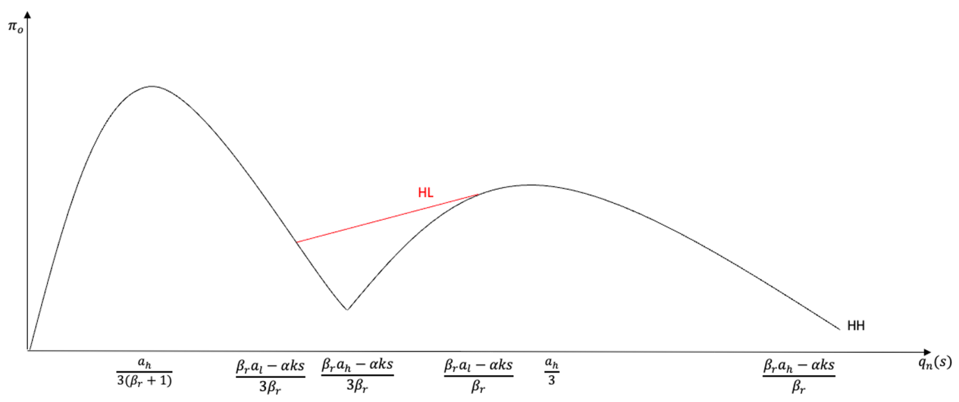
• First, we study how an OEM competes with an IR when information about the market size is available to both the OEM and IR. The specific aspects of competition studied are the decisions that the OEM and IR make about production quantity and quality levels and the decision that the IR makes about whether to encroach on the end market. For the latter, we find that the keys to the IR’s encroachment decision are its production cost advantage and the consumers’ preference for remanufactured products. The IR does not encroach on the market if its cost advantage and the consumers’ willingness to pay are low. When an IR’s cost advantage is moderate and the consumers’ willingness to pay is low, however, the IR encroaches on the market but does not remanufacture the full quantity available on the market (i.e., the quantity of products available for remanufacturing). When the IR’s cost advantage is high, the IR not only encroaches on the market but also remanufactures the full quantity available on the market. The OEM’s decisions about production quantity and quality levels also depend on the IR’s cost advantage and the consumers’ willingness to pay for the IR’s product. If the IR’s cost advantage and the consumers’ preference for the IR’s product are low, the OEM does not need to make adjustments to have the monopoly. If the IR’s cost advantage is moderate and the consumers’ willingness to pay for the IR’s product is low, the OEM can maintain the monopoly only if the OEM improves its product quality. If the OEM is unable to improve product quality sufficiently to deter IR encroachment, however, the OEM alters its quantity and quality based on the specific market conditions. If the consumers’ willingness to pay for the IR’s product is low and/or the IR’s cost advantage is low (high $\alpha$ and low ${\beta }_r$, which is explained in detail in Section 3), the OEM increases its product quality. If the consumers’ preference for the IR’s product is high and/or the IR’s cost advantage is high (low $\alpha$ and high ${\beta }_r$), the OEM reduces its production quantity to limit the available product that the IR can collect and remanufacture.
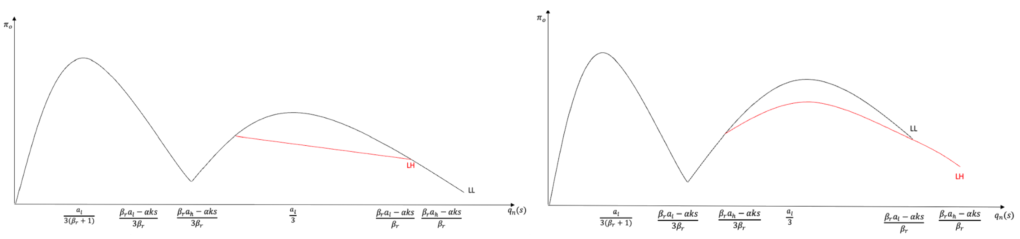
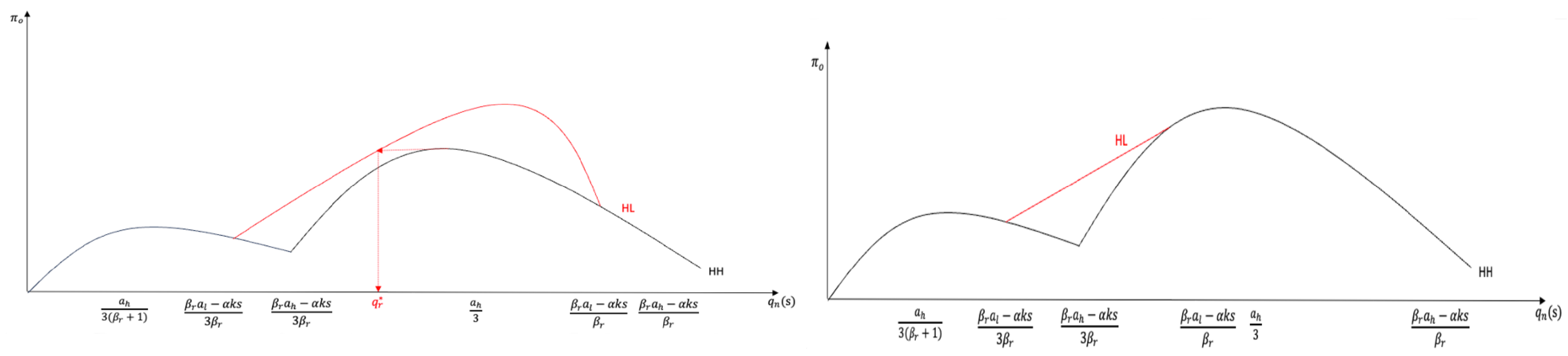
• Second, we model whether it is profitable for the OEM to share market information with the IR. We find that the OEM can benefit from sharing market information with the IR. When the market size is high, the OEM’s and IR’s optimal quantities are the same as in the benchmark model, where the OEM and IR have equal market information. Thus, hiding market information from the IR does not positively or negatively impact the OEM. However, when the market size is low, the OEM’s decision to hide market information from the IR hurts the OEM’s profits. To understand why, note that if the market size is low and the OEM does not share market information, the OEM’s optimal decision is to substantially reduce its production quantity to prevent the IR from encroaching on the market. If the OEM shares market information with the IR, however, its production quantity is higher than the quantity when information is not shared, even with IR encroachment. Hence, it is in the OEM’s interest to share market information with the IR when the market size is low.
• Third, we study how IR remanufacturing decisions affect consumer surplus, social surplus, and environmental impact. We find that consumer surplus increases when the IR engages in remanufacturing, while social surplus increases only when either the OEM’s or IR’s product is strongly favored. Additionally, we find that IR encroachment always has lower environmental impact due to two reasons. First, remanufacturing’s use of most of the original components decreases its environmental impact. Second, if the IR encroaches on the market, the OEM lowers its own production quantity to limit the availability of products for the IR to remanufacture. Hence, when the IR encroaches on the market, the lower overall production quantity results in a lower environmental impact.

In summary, our papers aims to shed some light on the impact of remanufacturing on environmental and economic sustainability.

The rest of this paper is structured as follows: Section 2 provides an overview of the related literature, highlighting the distinctive features and contributions of our work. Our model and assumptions are detailed in Section 3. The results in Section 4.1 outline the equilibrium for the benchmark model, where information is available to both the IR and the OEM. Section 4.2 and Section 4.3 discuss the asymmetric information case, where only the OEM has knowledge of the true market size and the IR uses a threshold quantity to infer the actual market size. In Section 5, we explore the socioeconomic benefit and policy implications. Specifically, we study the impact of the IR’s encroachment decision on consumer and social welfare, as well as its effects on the total environmental impact. Section 6 concludes with a summary of the paper and outlines potential directions for future research. All mathematical proofs are provided in Appendix A.

2. Literature Review

Our paper is closely related to two groups of literature studies, i.e., product remanufacturing and information asymmetry.

2.1. Remanufacturing

Product remanufacturing has received a great amount of attention in the operations literature. Models differ in whether remanufacturing is executed by a sole monopolist (e.g., Ferguson and Toktay [3], Ferrer and Swaminathan [4], Ferrer and Swaminathan [5]) or by an OEM and an IR in competition (e.g., Örsdemir et al. [6], Huang et al. [7], Wu and Wu [8], Wu [9]). In Ferguson and Toktay [3], the authors analyze the competition between new and remanufactured products produced by a monopolist manufacturer and identify conditions under which the monopolist would choose not to remanufacture its products. They then utilize a two-period game theoretical model to characterize the potential profit loss due to IR encroachment and analyze two entry deterrence strategies: in-house remanufacturing and preemptive collection. Aligned with their study, our work considers the circumstances that make it beneficial for an OEM to share market information with a competing IR.

Ferrer and Swaminathan [4] also study a monopolist which makes new products in the first period and offers both remanufactured and new products in future periods. The study finds that when remanufacturing profitability exceeds a threshold, it is beneficial for the monopolist to partially forgo the first-period margin by lowering the purchase price and selling additional units to increase the number of products available for remanufacturing in future periods. Under a duopoly with an IR competitor, this strategy is less appealing, because the competitor uses some of the additional units. Different from their findings, our results suggest that given its information advantage, this strategy could still be beneficial for the OEM.

Ferrer and Swaminathan [5] analyze the monopoly environment in two-period, multi-period (three, four, and five), and infinite planning horizons and characterize the optimal remanufacturing and pricing strategy for a firm. One of their takeaways, contrary to intuition, is that in a finite-horizon, multi-period setting, the optimal policy is not necessarily monotone in remanufacturing savings.

Among studies that model competition between an OEM and an IR in the base case, Örsdemir et al. [6] study how the competition between an IR and an OEM influences the total environmental impact and social welfare. In their study, the OEM also has the option of remanufacturing itself. The authors find that increasing the total amount of remanufacturing improves the environmental impact when the remanufacturing is performed by the OEM, but paradoxically, under certain circumstances, it actually worsens the impact when remanufacturing is performed by the IR. This is because competition increases the total quantity sold. Our work builds upon the framework used in this study to incorporate the effects of information asymmetry on OEM and IR relations.

In another study (Huang et al. [7]), IRs enter the market and compete with OEMs who only make new products and do not know the IRs’ cost of remanufacturing. The paper investigates incentives for IRs to share their cost information with OEMs. In their study, the authors note that the remanufactured product’s quantity is constrained by the new product’s quantity. If the new production cost is low enough such that the remanufactured product’s optimal quantity is less than the new product’s optimal quantity, the IR should always share cost information with the OEM so that the OEM’s quantity decisions at equilibrium are more responsive to market conditions to avoid overproduction or underproduction. However, if the remanufactured product’s optimal quantity is greater than the new product’s optimal quantity, the IR should not always share cost information. In this case, cost information sharing can allow the OEM to adjust the new product’s quantity to limit remanufacturing and hence be detrimental to the IR’s profits. When the IR does not voluntarily share cost information, they find that the environment is negatively impacted. The authors suggest that the government promote information sharing and subsidize IRs under certain conditions. Similar to theirs, our work also concerns information-sharing decisions, but it is the OEM sharing market demand information rather than the IR sharing remanufacturing cost information.

Wu and Wu [8] investigate the competition between OEMs and IRs not only in sales but also in the collection of used items for remanufacturing. They consider four strategies: SS, SC, CS, CC. S represents the economies of remanufacturing driven by sales, where the firm optimizes the price decision for sales and thus collects a sufficient quantity of used products to meet the demand of remanufacturing. C represents the economies of remanufacturing driven by collection, where the firm remanufactures all the collected used products that are acquired without the reward mechanism and thus makes a price decision subject to the collected quantity. This paper uses the consumer utility function regarding purchases and provides insights into how an OEM should respond to changes in competitive scenarios by allocating sales between new and OEM-remanufactured products.

Extending beyond OEMs and IRs, Wu [9] studies a supply chain where there is one manufacturer, one remanufacturer, and one retailer. Both manufacturers can invest in their product services and sell their products to this common retailer. In addition, the remanufacturer can invest in manufacturing cost saving. This paper identifies the equilibrium characteristics with respect to the remanufacturer’s effort spent on cost reduction, and price and service decisions for all members of the supply chain.

2.2. Information Asymmetry

Information asymmetry has been studied for many years in the supply chain literature in various settings. Rather than reporting the ample amount of literature, we focus our attention on the papers that include supplier encroachment. Li et al. [10] consider the case where the retailer is better informed than the supplier. The launch of the supplier’s direct self-branded product results in costly signaling behavior towards the retailer, as a result of which the retailer reduces its order quantity when the market size is small. Such a downward order distortion can amplify double marginalization. As a result, in addition to the “win–win” and “win–lose” outcomes for the supplier and the retailer, supplier encroachment can also lead to “lose–lose” and “lose–win” outcomes, particularly when the retailer has a significant efficiency advantage in the selling process and the prior probability of a large market is low.

Li et al. [10] jointly consider asymmetric information and nonlinear pricing effects within the context of supplier encroachment. The authors find that nonlinear pricing cannot mitigate double marginalization. In addition, apart from the downward distortion effect, upward distortion may also occur when the retailer purchases more than the efficient quantity.

Huang et al. [7] examine a retailer’s incentive to share information about market demand with a supplier who may encroach on the market. The study finds that the retailer may voluntarily share demand information in anticipation of supplier encroachment if demand is low, since this would discourage encroachment.

This paper addresses the knowledge gap of how asymmetric information affects encroachment decisions for an Independent Remanufacturer (IR) that is in competition with an OEM and models the circumstances for which it is beneficial for an OEM to share information with an encroaching IR. These analyses are distinct from those used in the four papers most closely related to our work. Huang et al. [7] and Örsdemir et al. [6] focus on the competition between OEMs and IRs. In Örsdemir et al. [6], the market is purely competitive between the OEM’s original product and an IR’s remanufactured product. Their model also allows the OEM to determine the quality and quantity of their new product. Specifically, the IR and OEM simultaneously make quantity and quality decisions. In our work, this is not the case. In reality, an IR makes production decisions after an OEM’s decisions (i.e., it tries to learn the information about the market that the OEM knows to estimate its own production quantity and quality). Thus, our work is a realistic extension where the IR makes decisions after the OEM. Huang et al. [7] incorporate a different aspect of asymmetric information in their model, where the IR knows the production costs for remanufacturing products more accurately than the OEM does. The authors show when it is beneficial for the IR to share information with the OEM. Our work focuses on the converse, i.e., when it is beneficial for an OEM to share market information with an IR. Li et al. [10] and Zhang et al. [11] discuss manufacturer encroachment and quality decision under asymmetric demand information conditions. These two papers focus on asymmetric information in the context without independent remanufacturing.

Building upon the aforementioned literature, our research questions address the gap about when it is beneficial for an OEM to share private demand information about the market it has with an IR and whether asymmetric information about the market always hurts an IR’s profits. To address our research questions, we use game theoretical modeling with two cases. The main model considers the case where an OEM sells a new product and remanufacturing is performed solely by an IR. Importantly, only the OEM knows the true market size, and the IR must make a guess of the market size with a fixed probability of guessing it right.

We compare the main model against a benchmark case where the OEM’s new product competes with the IR’s remanufactured product, when both parties know the true market size (full information case) and when neither party has information about the market (no information case). This comparison helps us to understand the effects of competition, the OEM’s and IR’s information management, and the IR’s encroachment decisions.

3. Model Notations and Assumptions

We assume that an Original Equipment Manufacturer (OEM, hereafter referred to as he) produces and sells a brand-new product. The OEM can determine the product quality level, which in turn affects demand. An Individual Remanufacturer (IR, hereafter referred to as she) collects used products sold by the OEM and then remanufactures and resells them to consumers. The decisions of the OEM concern the quantity ($q_n$) and quality levels (s) of the new product, and the decision of the IR concerns the quantity of the old product to collect from consumers for remanufacturing ($q_r$). We consider a single-period model with some assumptions below. Note that all these assumptions are either reasonable or found in the literature.

Assumption 1.

Producing a remanufactured product is less costly than manufacturing a new one.

This assumption is justified by the anticipated savings that arise from remanufacturing, i.e., not needing to buy raw materials nor complex machines/labor to convert them into finished products. Forgoing the conversion of raw materials into components also reduces energy costs.

Assumption 2.

The IR’s collection cost of old products is negligible. (This is a common assumption in the remanufacturing literature [3,12,13,14,15,16]).

Assumption 3.

The quantity of products remanufactured ($q_r$) is no more than the quantity of new products manufactured ($q_n$).

This assumption is reasonable, as the IR cannot collect more than what is available on the market.

Assumption 4.

Similar to the assumption proposed by Örsdemir et al. [6], Atasu and Souza [17], and Ferguson and Toktay [3], all cores of the collected products are in good enough shape and can be remanufactured. Therefore, the IR, if willing to, is able to recollect all the products that the OEM manufactured.

Assumption 5.

The price that consumers are willing to pay for the remanufactured product is a fraction of the new product’s price. (${\beta }_r$ is the remanufactured product price divided by the new product’s price; ${\beta }_r\in (0,1)$).

This assumption reflects consumers’ view that the remanufactured product has inferior quality compared with the brand-new product.

Assumption 6.

In this single-period model, old products can only be remanufactured once. (See [14,16]).

Assumption 7.

The market size ($a_i$) can only have two distinct values: high size ($a_i=a_h$) or low size ($a_i=a_l$) [18].

All the notations are summarized in

Table A1. Summary of notations.

Symbol	Definition
$a_h$,$a_l$	The market bases for high market and low market, respectively
$\alpha$	Manufacturing cost efficiency of the IR
${\beta }_r$	Consumers’ willingness to pay for the remanufactured product
s	Quality level of the product
$p_n$,$p_r$	Prices made by the OEM and IR, respectively
k	Scaling parameter
${\pi }_o$,${\pi }_R$	Profit functions of the OEM and IR, respectively
$q_n$,$q_r$	Demand functions of the OEM and IR, respectively

in Appendix A. The game sequence is as follows:

• The OEM determines the new product’s quantity and quality levels and starts selling the product.
• The IR collects products from the market and resells them to consumers.
• The market clearing price is realized. The profits of the OEM and IR are realized.

We adopt the following linear price functions for the OEM’s and IR’s new and remanufactured products [6,16,19]:

$$\begin{array}{c}\hfill p_n=s(a_i-q_n-{\beta }_r{q}_r)\end{array}$$

(1)

$$\begin{array}{c}\hfill p_r={\beta }_{r}s(a_i-q_n-q_r)\end{array}$$

(2)

In Equations (1) and (2), s is the quality level of the brand-new product determined by the OEM. A higher s indicates a higher quality level and thus a higher price. ${\beta }_r\in (0,1)$ is regarded as the discount in the consumers’ willingness to pay for the remanufactured product compared with the brand-new product and measures the degree of inferiority of the remanufactured product. As ${\beta }_r$ increases, the remanufactured product’s price increases, and the brand-new product’s price decreases. If ${\beta }_r=1$, then the two products are identical.

As there is only one period, the profit functions for the OEM and IR are given in Equations (3) and (4). The unit variable cost of producing a new product with a quality level of s is $k{s}^2$ for the OEM. The IR’s unit production is cheaper, as we discussed earlier in Assumption 4. Thus, the IR’s unit variable cost is $\alpha k{s}^2$, where $\alpha <1$, and represents the IR’s cost advantage, diminishing as $\alpha$ gets closer to one.

$$\begin{array}{c}\hfill \underset{q_n,s}{max}{\pi }_{OEM}[q_n,s]=p_n{q}_n-k{s}^2{q}_n,\mathrm{s}.\mathrm{t}.q_n\ge 0\end{array}$$

(3)

$$\begin{array}{c}\hfill \underset{q_r}{max}{\pi }_{IR}\left[q_r\right|(q_n,s)]=p_r{q}_r-\alpha k{s}^2{q}_r\mathrm{s}.\mathrm{t}.q_r\ge 0,q_n\ge q_r\end{array}$$

(4)

In the main model, only the OEM knows the market size ($a_i$). To study the impact of asymmetric information, we start from two benchmark cases: in the first case (full information), both the OEM and the IR know the market size ($a_i$), and in the second case (no information), neither knows the market size.

4. Results

4.1. Analysis of Benchmark Model: Full Information

In the full information case, both the OEM and the IR know market size information. The model is solved backward, and the equilibrium quantities and quality for the OEM and IR are summarized in Proposition 1, where $q_n$ is the OEM’s equilibrium quantity, $q_r$ is the IR’s equilibrium quantity, and s is the equilibrium quality. Lemma 1 shows that there can be four different types of equilibria, labeled as Regions A, B, C, and D. In Regions A and B, the IR production quantity is zero, which means that the OEM is a monopolist. In Region A, the OEM does not factor the IR into his quantity and quality decisions at all, while in Region B, the OEM has to increase his quality to keep the IR out of the market. In Regions C and D, the OEM cannot keep the IR out of the market. In Region C, the IR only remanufactures a fraction of the available products on the market, while in Region D, the IR remanufactures all of the available products on the market. Which region the equilibrium falls into depends on the IR’s cost advantage, $\alpha$, and the consumers’ willingness to pay for the remanufactured product, ${\beta }_r$. The conditions are also characterized in Proposition 1.

Proposition 1.

In the full information case, the following is a summary of the decisions for the OEM and IR in each region:

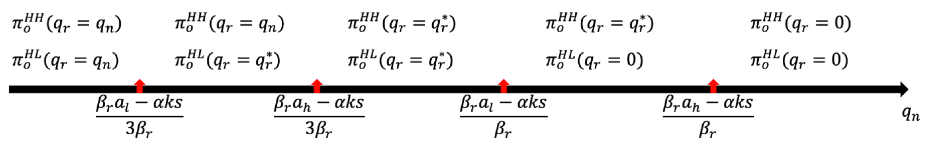
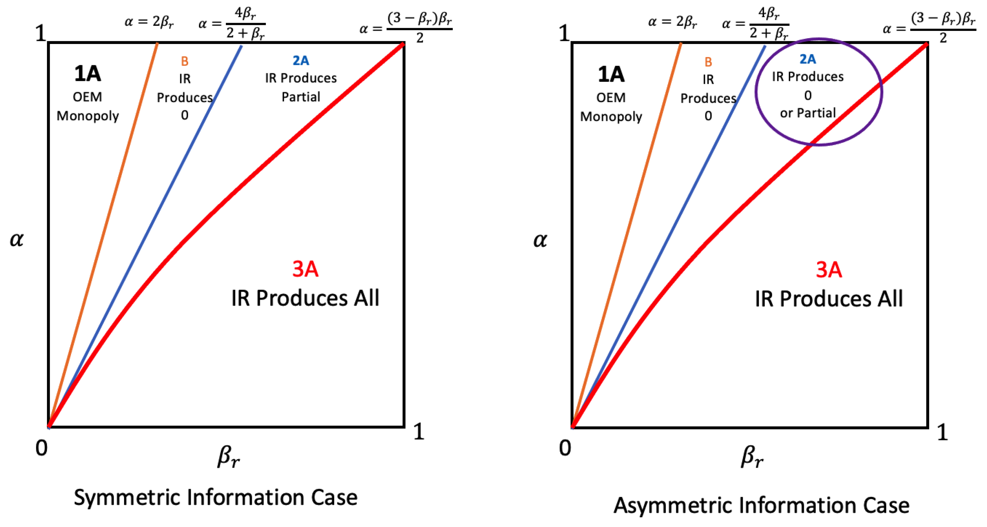
• When $\alpha \in \left(min\left\{2{\beta }_r,1\right\},1\right)$, denoted as Region A, the OEM is a monopolist, and the IR does not encroach on the market; the OEM’s and IR’s optimal quantities are $q_n={\displaystyle \frac{a_i}{3}}$, $s={\displaystyle \frac{a_i}{3k}}$, and $q_r=0$.
• When $\alpha \in \left(min\left\{{\displaystyle \frac{4{\beta }_r}{2+{\beta }_r}},1\right\},min\left\{2{\beta }_r,1\right\}\right)$, denoted as Region B, the IR does not encroach on the market, and the OEM’s and IR’s optimal quantities are $q_n={\displaystyle \frac{a_i}{3}}$, $s={\displaystyle \frac{2a_i{\beta }_r}{3k\alpha }}$, and $q_r=0$.
• When $\alpha \in \left(min\left\{{\displaystyle \frac{(3-{\beta }_r){\beta }_r^2}{2}},1\right\},min\left\{{\displaystyle \frac{4{\beta }_r}{2+{\beta }_r}},1\right\}\right)$, denoted as Region C, the IR remanufactures part of the available products, and the OEM’s and IR’s optimal quantities are $q_n={\displaystyle \frac{a_i}{3}}$, $s={\displaystyle \frac{a_i(2-{\beta }_r)}{3k(2-\alpha )}}$, and $q_r={\displaystyle \frac{a_i(4{\beta }_r-2\alpha -\alpha {\beta }_r)}{6{\beta }_r(2-\alpha )}}$.
• When $\alpha \le min\left\{{\displaystyle \frac{(3-{\beta }_r){\beta }_r^2}{2}},1\right\}$, denoted as Region D, the IR remanufactures all available products, and the OEM’s and IR’s optimal quantities are $q_n={\displaystyle \frac{a_i}{3({\beta }_r+1)}}$, $s={\displaystyle \frac{a_i}{3k}}$, and $q_r={\displaystyle \frac{a_i}{3({\beta }_r+1)}}$.

Figure 1 graphically depicts the equilibrium regions. In this plot, the vertical axis is the IR’s cost advantage ($\alpha$), and the horizontal axis is the consumers’ willingness to pay for the IR’s product (${\beta }_r$). Three critical transition lines divide the plane into four regions. If the IR’s cost advantage is low (that is, $\alpha$ is close to one), and the consumers’ willingness to pay is low (that is, ${\beta }_r$ is close to zero), a pure monopoly arises, where the OEM does not consider the IR in his production decisions. Region B is defined by a moderate cost advantage with low consumer willingness to pay. In this region, the OEM still keeps the IR out of the market, but he has to improve his quality to do so. When the IR’s cost advantage is moderate and the consumers’ willingness to pay is low, the equilibrium falls in Region C. In this region, the IR encroaches on the market, but she does not produce the full quantity available on the market. When the IR cost advantage is high, the IR not only encroaches on the market but also produces the full quantity available on the market, which is Region D. Clearly, a lower $\alpha$ and a higher ${\beta }_r$ imply a more competitive IR, encouraging a more aggressive encroachment decision.

4.2. Analysis of Benchmark Model: No Information

In the case of no information, neither the OEM nor the IR has information about the market size. In such a case, the market size ($a_i$) is assumed to be random ex ante and can be either high ($a=a_h$) with probability p or low ($a=a_l$) with probability $1-p$, where $a_h>a_l>0$. Therefore, the expected market size ($\mu$) is given as $\mu =p{a}_h+(1-p)a_l$. Both firms maximize their expected profits.

$$\begin{array}{c}\hfill \underset{q_n,s}{max}{\pi }_{OEM}[q_n,s]=\mathrm{E}[p_n{q}_n-k{s}^2{q}_n],\mathrm{s}.\mathrm{t}.q_n\ge 0\end{array}$$

(5)

$$\begin{array}{c}\hfill \underset{q_r}{max}{\pi }_{IR}\left[q_r\right|(q_n,s)]=\mathrm{E}[p_r{q}_r-\alpha k{s}^2{q}_r],\mathrm{s}.\mathrm{t}.q_r\ge 0,q_n\ge q_r\end{array}$$

(6)

We solve for $q_r$, $q_n$, and s in similar ways as in the full information case and obtain similar results. The equilibrium quantities and quality can also be characterized into four regions, as summarized in

Table 1. Competition in remanufacturing when information is unknown: equilibrium for quantity and quality.

Region	${\mathit{q}}_{\mathit{n}}$	s	${\mathit{q}}_{\mathit{r}}$
A—OEM monopoly	${\displaystyle \frac{\mu }{3}}$	${\displaystyle \frac{\mu }{3k}}$	0
B—The IR produces 0	${\displaystyle \frac{\mu }{3}}$	${\displaystyle \frac{2\mu {\beta }_r}{3k\alpha }}$	0
C—The IR produces partial quantity	${\displaystyle \frac{\mu }{3}}$	${\displaystyle \frac{\mu (2-{\beta }_r)}{3k(2-\alpha )}}$	${\displaystyle \frac{\mu (4{\beta }_r-2\alpha -\alpha {\beta }_r)}{6{\beta }_r(2-\alpha )}}$
D—The IR produces all quantity	${\displaystyle \frac{\mu }{3({\beta }_r+1)}}$	${\displaystyle \frac{\mu }{3k}}$	${\displaystyle \frac{\mu }{3({\beta }_r+1)}}$

.

4.3. Asymmetric Information Model

In this section, we discuss the asymmetric information scenario where the IR does not know the actual market size. This is realistic in practice when an IR is new to the market and does not have previous experience in selling products to consumers. The OEM, in contrast, can draw on his years of experience selling products to assess market demand accurately. The game sequence for the asymmetric information model is the following:

• The OEM, observing the market size, sets his production quantity and product quality levels.
• Using the OEM’s production quantity as a signal of market size, the IR decides the quantity of used products to remanufacture.
• The market clearing price is realized. The profits of the OEM and the IR are realized.

Following Örsdemir et al. [6], the OEM’s and IR’s price functions for new and remanufactured products are

$$\begin{array}{c}\hfill p_n=s(a_i-q_n-{\beta }_r{q}_r)\end{array}$$

(7)

$$\begin{array}{c}\hfill p_r={\beta }_{r}s(a_i-q_n-q_r)\end{array}$$

(8)

$$\begin{array}{c}\hfill \underset{q_n,s}{max}{\pi }_{OEM}[q_n,s|a_i]=p_n{q}_n-k{s}^2{q}_n,\end{array}$$

(9)

$$\begin{array}{c}\hfill \mathrm{s}.\mathrm{t}.q_n\ge 0\end{array}$$

(10)

$$\begin{array}{c}\hfill \underset{q_r}{max}{\pi }_{IR}\left[q_r\right|(q_n,s),\overline{a_i}]=p_r{q}_r-\alpha k{s}^2{q}_r\end{array}$$

(11)

$$\begin{array}{c}\hfill \mathrm{s}.\mathrm{t}.q_r\ge 0,q_n\ge q_r\end{array}$$

(12)

As with the benchmark case, we use the same linear functions for the prices and profits. However, while they remain the same, the optimal response functions for the IR are different from the benchmark cases. This is because the IR makes her decisions based on her deduction of the market size using the OEM’s quantity as a signal, rather than on the true market size. Although the IR does not know the true market size, she can make rational inferences about it according to the OEM’s production quantity ($q_n$). A larger production quantity signals a larger market size to the IR, who thus produces more. However, based on basic supply/demand, a larger number of products on the market imposes negative pressure on the product’s price. Therefore, the OEM prefers the IR to sell a lower quantity of remanufactured products, $q_r$, allowing for a higher price for brand-new products. Therefore, if the OEM knows that the market size is high, in which case he is referred to as a high-type OEM, he has an incentive to pretend that the market size is low, i.e., to be a low-type OEM. This may deceive the IR into believing that the market is low, resulting in a lower $q_r$ and a higher market price for the OEM. However, the distortions in quantity that arise from a high-type OEM pretending to be a low-type OEM also hurt the low-type OEM’s profit due to a reduced number of products sold. The low-type OEM then wants to separate himself from the high-type OEM to prevent the high-type OEM from successfully mimicking a low-type OEM. A separating equilibrium thus arises.

From Equation (11), the IR forms a belief ($\overline{a_i}$) regarding the market size, which depends on the OEM’s selling quantity ($q_n$). In a separating equilibrium, the IR believes that there exists a threshold quantity ($q_r^s$), such that if $q_n>q_r^s$, the IR believes that $\overline{a_i}=a_h$, while if $q_n<q_r^s$, the IR believes that $\overline{a_i}=a_l$. Such a Perfect Bayesian Separating Equilibrium (PBSE) exists if and only if the OEM’s quantity decision ($q_n$) satisfies

$$\begin{array}{c}\hfill max{\pi }_n(q_n>q_r^s|a_h)\ge max{\pi }_n(q_n\le q_r^s|a_h)\end{array}$$

(13)

$$\begin{array}{c}\hfill max{\pi }_n(q_n\le q_r^s|a_l)\ge max{\pi }_n(q_n>q_r^s|a_l)\end{array}$$

(14)

$$\begin{array}{c}\hfill q_r^s\ge 0\end{array}$$

(15)

Inequality (13) ensures that the OEM pretending to be a low type when the market is high hurts his profit. Likewise, Inequality (14) means that the OEM pretending to be a high type when the market is low is also worse off. The last inequality guarantees that the OEM’s production quantity is non-negative.

On the other hand, when the high-type OEM successfully mimics low-type decisions, a pooling equilibrium arises. In a pooling equilibrium, both high-type and low-type OEMs manufacture the same quantities. In this paper, we do not discuss the pooling equilibrium, since according to Zhang et al. [11], no pooling equilibrium survives the intuitive criterion proposed by Cho and Kreps [20].

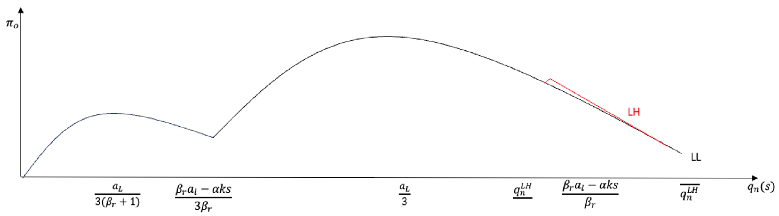
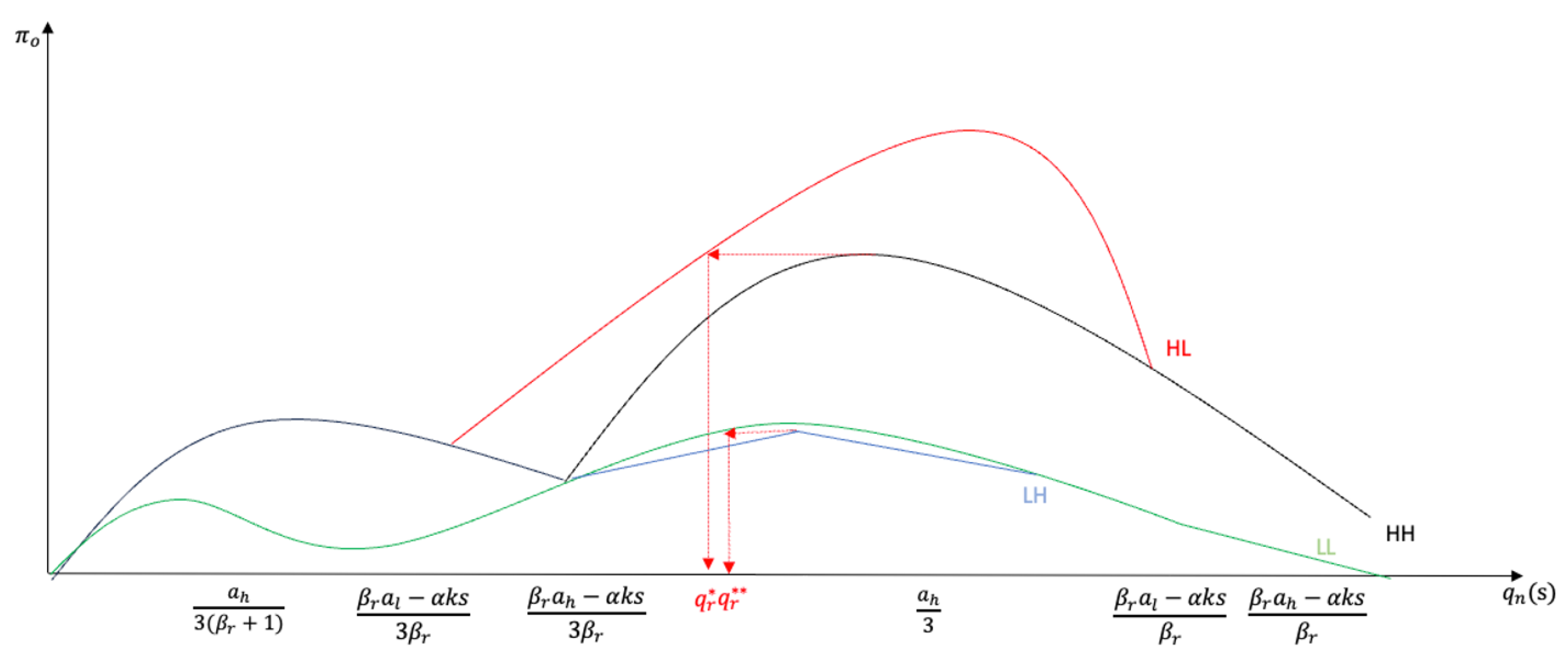
4.4. Analysis of Asymmetric Information Model

We then solve for the separating equilibrium given these inequality constraints. We report the equilibrium results below in Proposition 2. Briefly, when the market size is high, the OEM’s and IR’s optimal quantities in this separating equilibrium are the same as those obtained from the benchmark model, where the OEM and the IR have equal information. Profits are thus the same for the symmetric and asymmetric information cases, and the OEM does not benefit from having an information advantage.

When the market size is low, under certain market circumstances, the OEM’s profit is less in the asymmetric information case than in the symmetric information case. Thus, under these circumstances, the OEM benefits from sharing market information. Under other circumstances, the OEM’s profits are the same for the symmetric and asymmetric cases.

Proposition 2.

In the presence of asymmetric information, the following is a summary of the equilibrium results for the OEM and IR:

• When the market size is high, i.e., $a_i=a_h$, the OEM’s and IR’s optimal quantities are those obtained from the benchmark model above, when the OEM and IR have equal information. Thus, it is sensible for the OEM to share his market information with the IR.
• When the market size is low, i.e., $a_i=a_l$, the OEM may make different decisions from the benchmark model. The detailed strategy depends on model parameters and is listed in

  Table 2. Competition in remanufacturing: separating equilibrium for quantity and quality when the market is low.

  Region	${\mathit{q}}_{\mathit{n}}$	s	${\mathit{q}}_{\mathit{r}}$
  A—OEM monopoly	${\displaystyle \frac{a_l}{3}}$	${\displaystyle \frac{a_l}{3k}}$	0
  B—The IR produces 0	${\displaystyle \frac{a_l}{3}}$	${\displaystyle \frac{2a_l{\beta }_r}{3k\alpha }}$	0
  C—The IR produces 0 or partial quantity	$min\left\{{\displaystyle \frac{a_l}{3}},\widehat{q_r^s}\right\}$	${\displaystyle \frac{a_l(2-{\beta }_r)}{3k(2-\alpha )}}$ or ${\displaystyle \frac{{\beta }_r(a_l-\widehat{q_r^s})}{\alpha k}}$	${\displaystyle \frac{a_l(4{\beta }_r-2\alpha -\alpha {\beta }_r)}{6{\beta }_r(2-\alpha )}}$ or 0
  D—The IR produces all quantity	${\displaystyle \frac{a_l}{3({\beta }_r+1)}}$	${\displaystyle \frac{a_l}{3k}}$	${\displaystyle \frac{a_l}{3({\beta }_r+1)}}$

  .

Focusing on the case when the market size is low, the equilibrium quantities and product quality can be characterized in a similar way as in the benchmark case, i.e., there exist four regions, as summarized in Table 2. Note that for three of the regions, the results are equivalent to the benchmark case with symmetric information. However, Region C is different. This is the region where the IR’s cost advantage is moderate and the consumers’ willingness to pay for the IR’s product is low. In this region, if the market size (${\displaystyle \frac{a_l}{3}}$) is smaller than the IR’s quantity threshold for inferring the market size, then the equilibrium results match the benchmark case. However, if the IR’s quantity threshold is smaller than ${\displaystyle \frac{a_l}{3}}$, then the IR does not encroach on the market (her quantity ($q_r$) is zero). In this scenario, the OEM’s quantity is smaller than the benchmark quantity, and his profits are hurt. Thus, in this scenario, it benefits the OEM to share his market information with the IR.

Figure 2 below is a graphical comparison of the symmetric and asymmetric information cases. They are very similar, except for special circumstances in Region C, where the IR may choose not to encroach on the market, which hurts the profits of the OEM, even though the OEM effectively has a monopoly. The reason why the OEM’s profits are hurt in this special case is because he decreases his quantity to deter the IR from encroaching on the market, and the cost from the reduced quantity outweighs the gains in price from the OEM being a monopoly.

We further examine profit in the scenarios of full information, no information, and asymmetric information. We incorporate equilibrium quantity and quality levels from Proposition 1 and Table 2 into the expected profit for the OEM, expressed as follows: ${\pi }_{OEM}=\mathrm{E}[p_n{q}_n-k{s}^2{q}_n]=p[p_n^H{q}_n-k{s}^2{q}_n]+(1-p)[p_n^L{q}_n-k{s}^2{q}_n]$. The OEM’s profit in the no information case is determined by utilizing the equilibrium data from Table 1 and plugging them into the profit function: ${\pi }_{OEM}=p_n{q}_n-k{s}^2{q}_n$.

Proposition 3.

Profit for the OEM is lower in the no information scenario. Comparing the full information and asymmetric information scenarios, when the market size is low, the expected quantity and profit of the OEM are higher in the full information case; when the market size is high, the OEM’s profits are equivalent in both cases.

Propositions 2 and 3 show how the IR can decide whether to encroach on the market or not based on her production cost advantage and the consumers’ preference for her products. In addition, the OEM can use the IR’s production cost advantage and the consumers’ preference for remanufactured products to decide (a) the quantity and quality of his own product to deter IR encroachment and (b) whether it is beneficial to share his information with the IR.

5. Discussion on Socioeconomic Benefit and Policy Implications

5.1. Consumer and Social Welfare

In this section, we investigate how remanufacturing affects consumer surplus and ($CS$) and social surplus ($SS$). Consumer surplus is written as

$$CS={\int }_{a_i-q_n-q_r}^{a_i-q_n}(\beta \theta s-p_r)d\theta +{\int }_{a_i-q_n}^{a_i}(\theta s-p_n)d\theta$$

(16)

The first part in Equation (16) is the surplus from remanufacturing products, and the second part is the surplus from new products sold. Social surplus is the sum of consumer surplus and firm profits. Given the relative similarity between the case with asymmetric information and the base model, we will focus solely on the base model scenario. The equilibrium quality, new and remanufactured product quantities, and consumer and social surpluses are summarized in

Table 3. Competition in remanufacturing: equilibrium for quantity, quality, and consumer and social surpluses.

Region	${\mathit{q}}_{\mathit{n}}$	s	${\mathit{q}}_{\mathit{r}}$	$\mathit{CS}$	$\mathit{SS}$
A	${\displaystyle \frac{a_i}{3}}$	${\displaystyle \frac{a_i}{3k}}$	0	${\displaystyle \frac{a_i^3}{54k}}$	${\displaystyle \frac{a_i^3}{18k}}$
B	${\displaystyle \frac{a_i}{3}}$	${\displaystyle \frac{2a_i{\beta }_r}{3k\alpha }}$	0	${\displaystyle \frac{{\beta }_r{a}_i^3}{27\alpha k}}$	${\displaystyle \frac{{\beta }_r(5\alpha -4{\beta }_r)a_i^3}{27{\alpha }^{2}k}}$
C	${\displaystyle \frac{a_i}{3}}$	${\displaystyle \frac{a_i(2-{\beta }_r)}{3k(2-\alpha )}}$	${\displaystyle \frac{a_i(4{\beta }_r-2\alpha -\alpha {\beta }_r)}{6{\beta }_r(2-\alpha )}}$	${\displaystyle \frac{(2-{\beta }_r)a_i^3}{108{(2-\alpha )}^3{\beta }_{r}k}}{{\rm Y}}_c$	${\displaystyle \frac{(2-{\beta }_r)a_i^3}{108{(2-\alpha )}^3{\beta }_{r}k}}{{\rm Y}}_s$
D	${\displaystyle \frac{a_i}{3({\beta }_r+1)}}$	${\displaystyle \frac{a_i}{3k}}$	${\displaystyle \frac{a_i}{3({\beta }_r+1)}}$	${\displaystyle \frac{(1+3{\beta }_r)a_i^3}{54{(1+{\beta }_r)}^{2}k}}$	${\displaystyle \frac{(1+3{\beta }_r)a_i^3}{54{(1+{\beta }_r)}^{2}k}}$

.

Here, ${{\rm Y}}_c=4{\alpha }^2+16\left[1-(3-\alpha )\alpha \right]{\beta }_r+(4-\alpha )(12-5\alpha ){\beta }_r^2$, ${{\rm Y}}_s=16{\beta }_r(1+7{\beta }_r)+{\alpha }^2\left[28+{\beta }_r(40+3{\beta }_r)\right]-48\alpha {\beta }_r(3+{\beta }_r)$.

$C{S}_B-C{S}_A=-{\displaystyle \frac{(\alpha -2{\beta }_r)a_i^3}{54\alpha k}}>0$ if ${\beta }_r>{\displaystyle \frac{\alpha }{2}}$. In Region B, the OEM has to increase the product quality to discourage the IR from entering the market, especially when consumers have a strong willingness to pay more for remanufactured products, i.e., when $2{\beta }_r>\alpha$. The better product quality in this region contributes to an augmentation in consumer surplus.

$$C{S}_C-C{S}_A={\displaystyle \frac{a_i^3}{108k}}\ast \left\{{\displaystyle \frac{(2-{\beta }_r)\left[4{\alpha }^2+16(1+{\alpha }^2-3\alpha ){\beta }_r+(\alpha -4)(5\alpha -12){\beta }_r^2\right]}{{\beta }_r{(2-\alpha )}^3}}-2\right\}.$$

Numerically, we can show that ${\displaystyle \frac{(2-{\beta }_r)\left[4{\alpha }^2+16(1+{\alpha }^2-3\alpha ){\beta }_r+(\alpha -4)(5\alpha -12){\beta }_r^2\right]}{{\beta }_r{(2-\alpha )}^3}}-2$ is positive when $\alpha ,{\beta }_r\in [0,1]$. Hence, $C{S}_C-C{S}_A>0$.

$C{S}_D-C{S}_A={\displaystyle \frac{(1-{\beta }_r){\beta }_r{\mu }^3}{54{(1+{\beta }_r)}^{2}k}}$ is always positive.

Proposition 4.

Compared with the case where the OEM monopolizes the market and the IR chooses not to encroach on the market (Region A), consumer surplus increases either when the OEM prevents IR encroachment through improved product quality (Region B), given that $\alpha \le 2{\beta }_r$, or when the IR is involved in remanufacturing (Regions C and D).

Proposition 4 explores how consumer surplus can benefit from the IR’s involvement in remanufacturing. Next, we study the impact of IR’s participation in remanufacturing on social surplus. Using the social surplus results from each region as presented in Table 3, we compare the values of social surplus between Region A and the other regions, as outlined below.

$S{S}_B-S{S}_A=-{\displaystyle \frac{(3\alpha -4{\beta }_r)(\alpha -2{\beta }_r)a_i^3}{54{\alpha }^{2}k}}$. It is negative, and social surplus in Region B is less than in Region A if ${\beta }_r<{\displaystyle \frac{\alpha }{2}}$ or ${\beta }_r>{\displaystyle \frac{3\alpha }{4}}$.

$S{S}_C-S{S}_A={\displaystyle \frac{a_i^3\left\{{\displaystyle \frac{(2-{\beta }_r)\left[16{\beta }_r(1+7{\beta }_r)+{\alpha }^2(28+40{\beta }_r+3{\beta }_r^2)-48\alpha {\beta }_r(3+{\beta }_r)\right]}{{\beta }_r{(2-\alpha )}^3}}-6\right\}}{108k}}$

$={\displaystyle \frac{a_i^3\left\{{\displaystyle \frac{(2-{\beta }_r){{\rm Y}}_s}{{\beta }_r{(2-\alpha )}^3}}-6\right\}}{108k}}$

Under certain conditions for ${\beta }_r\in (\underline{{\beta }_r},\overline{{\beta }_r})$, the expression ${\displaystyle \frac{(2-{\beta }_r){{\rm Y}}_s}{{\beta }_r{(2-\alpha )}^3}}-6$ becomes negative. This observation is illustrated in Figure 3. In the figure, the blue area represents 0, while the yellow area corresponds to ${\displaystyle \frac{(2-{\beta }_r){{\rm Y}}_s}{{\beta }_r{(2-\alpha )}^3}}-6$, which is part of the numerator of $S{S}_C-S{S}_A$. If ${\displaystyle \frac{(2-{\beta }_r){{\rm Y}}_s}{{\beta }_r{(2-\alpha )}^3}}-6$ is positive, then $S{S}_C-S{S}_A$ is positive; otherwise, $S{S}_C-S{S}_A$ is negative. Thus, Figure 3 visually depicts the conditions under which $S{S}_C-S{S}_A$ is positive or negative. The blue area serves as a representation of the value 0, aiding us in determining the specific conditions for $S{S}_C-S{S}_A$ to be positive or negative.

According to Figure 3, if ${\beta }_r$ falls within the range $(\underline{{\beta }_r},\overline{{\beta }_r})$, the expression ${\displaystyle \frac{(2-{\beta }_r){{\rm Y}}_s}{{\beta }_r{(2-\alpha )}^3}}-6$ is negative, resulting in a larger social surplus in Region A compared with Region C.

$S{S}_D-S{S}_A={\displaystyle \frac{(3{\beta }_r-2\alpha )a_i^3}{54(1+{\beta }_r)k}}$. If ${\beta }_r$ is less than ${\displaystyle \frac{2\alpha }{3}}$, the difference $S{S}_D-S{S}_A$ is negative, indicating that the social surplus in Region A surpasses that in Region D.

Proposition 5.

There exist thresholds, specifically when ${\beta }_r<{\displaystyle \frac{\alpha }{2}}$, ${\beta }_r>{\displaystyle \frac{3\alpha }{4}}$, ${\beta }_r\le \underline{{\beta }_r}$, or ${\beta }_r\ge min\{{\displaystyle \frac{2\alpha }{3}},\overline{{\beta }_r}\}$, where social surplus is higher when the IR chooses to encroach on the market and engage in remanufacturing (Regions B, C, and D) than in the case where the OEM has a monopoly on the market (Region A).

From Propositions 4 and 5, consumer surplus is higher when the IR chooses to encroach on the market and engage in remanufacturing. However, this is not the case for social surplus. Social surplus increases only when ${\beta }_r<{\displaystyle \frac{\alpha }{2}}$, ${\beta }_r>{\displaystyle \frac{3\alpha }{4}}$, ${\beta }_r\le \underline{{\beta }_r}$, or ${\beta }_r\ge min\{{\displaystyle \frac{2\alpha }{3}},\overline{{\beta }_r}\}$. This implies that either the OEM’s product has to be highly favored or the IR’s product has to be highly favored for the social surplus to increase when the IR encroaches on the market and engages in remanufacturing.

5.2. Environmental Impact

In this section, we explore the environmental impact of both new and remanufactured products. We assume that one unit of a new product and a remanufactured product incur environmental impacts denoted by E and e, respectively. Therefore, when the OEM produces $q_n$ units and the IR produces $q_r$ units, the total environmental impact is given by $q_{n}E+q_{r}e$.

Table 4. Environmental impact.

Region	Environmental Impact	$\mathit{\alpha }$	${\mathit{\beta }}_{\mathit{r}}$
A	${\displaystyle \frac{E{a}_i}{3}}$	$Constant$	$Constant$
B	${\displaystyle \frac{E{a}_i}{3}}$	$Constant$	$Constant$
C	${\displaystyle \frac{a_i\left[2(2-\alpha ){\beta }_{r}E-2\alpha e+(4-\alpha ){\beta }_{r}e\right]}{6(2-\alpha ){\beta }_r}}$	↓	↑
D	${\displaystyle \frac{(E+e)a_i}{3(1+{\beta }_r)}}$	$Constant$	↓

provides a summary of the total environmental impact for each region and how the environmental impact depends on the relative IR cost advantage ($\alpha$) and the consumer perception of the remanufactured product (${\beta }_r$).

We compare the total environmental impacts between Regions A and C: $EI\left(A\right)-EI\left(C\right)={\displaystyle \frac{e{a}_i\left[\alpha (2+{\beta }_r)-4{\beta }_r\right]}{6(2-\alpha ){\beta }_r}}>0$ if ${\beta }_r<{\displaystyle \frac{2\alpha }{4-\alpha }}$.

We compare the total environmental impacts between Regions A and D: $EI\left(A\right)-EI\left(D\right)={\displaystyle \frac{{\beta }_{r}E{a}_i-e{a}_i}{3+3{\beta }_r}}>0$ if ${\beta }_r>{\displaystyle \frac{e}{E}}$.

Proposition 6.

• When the IR’s entry is deterred by the OEM (Region B), the environmental impact is the same as when the IR does not encroach on the market (Region A).
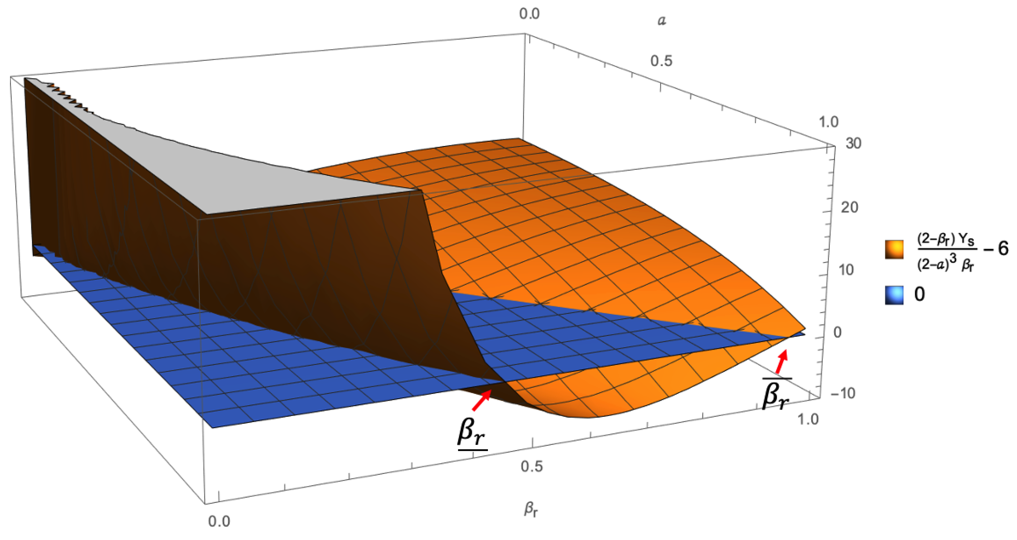
• When the IR enters the market but does not remanufacture all products on the market (Region C), the environmental impact is higher than when the IR does not encroach on the market (Regions A and B) if ${\beta }_r<{\displaystyle \frac{2\alpha }{4-\alpha }}$. Lower α and higher ${\beta }_r$ increase the environmental impact in Region C.
• When the IR enters the market and remanufactures all products on the market (Region D), the environmental impact is higher than when IR does not encroach on the market (Regions A and B) if ${\beta }_r>{\displaystyle \frac{e}{E}}$. A lower ${\beta }_r$ increases the environmental impact in Region D.

Proposition 6 shows that when the IR remanufactures in Region C, the environmental impact is sensitive to the IR production cost advantage, $\alpha$, and the consumers’ willingness to pay for the remanufactured product, ${\beta }_r$. When ${\beta }_r<{\displaystyle \frac{2\alpha }{4-\alpha }}$, e is smaller, and there is a smaller difference between $EI\left(A\right)$ and $EI\left(C\right)$, the IR encroaching on the market further reduces the environmental impact. When in Region D, the environmental impact is related to ${\displaystyle \frac{e}{E}}$. When the remanufacturer product has a small impact on the environment, with smaller ${\displaystyle \frac{e}{E}}$, the overall environmental impact decreases with IR encroachment.

We believe that remanufacturing has a lower environmental impact compared with manufacturing from scratch. This is because remanufacturing involves using more of the original shell and most of the original internal parts, resulting in a reduced environmental impact. Moreover, within the context of our study, the introduction of competition from an encroaching IR introduces additional complexity into the relationship. When the IR encroaches on the market, the overall production quantity may decrease, as the OEM tries to deter IR entrenchment by reducing production quantity, resulting in a limited pool of available products for the IR to collect. Hence, under specific conditions, an OEM monopoly may yield a higher total quantity, consequently leading to an increased total environmental impact.

6. Conclusions and Future Directions

In this research, we study the competition between an Original Equipment Manufacturer (OEM) and an Independent Remanufacturer (IR) and examine how their optimal decisions and profits are affected by asymmetric market size information. We show that the IR’s cost efficiency and the consumers’ willingness to pay for the IR’s product both strongly influence the OEM’s and IR’s production quantities and IR’s encroachment decisions. When the IR’s cost efficiency is very high, meaning that the production cost to remanufacture the same amount of product is low, the IR collects all the available products sold by the OEM for remanufacturing, while the OEM chooses to restrict his manufacturing of brand-new products. However, when the production efficiency or consumers’ willingness to pay is low, the IR chooses not to encroach on the market.

In addition, in the asymmetric information model, the low-type OEM (the OEM that knows that the market size is low) reduces his production quantity to falsely signal a lower market size when the IR’s cost efficiency is moderate. This prevents the IR from entering the market altogether. However, in case of a high-type OEM or if the IR’s cost efficiency is low or high, the OEM should share his information about the market with the IR to maximize his profits. We also find that the OEM always earns higher profits when both parties have full information, compared with no information or asymmetric information.

Our future research will aim to extend the asymmetric information case by considering the cost of obtaining asymmetric information. In addition, the model can be extended in the following two directions:

• The OEM sells both new and remanufactured products, and both parties know the true market size.
• The IR does not encroach on the market but instead sells the remanufactured products to the OEM under asymmetric information conditions.

These two cases could be useful to further understand the effects of information management between the OEM and IR, as well as the IR’s encroachment decisions.

References

- Remanufacturing, Inc. Available online: https://www.inc.com/encyclopedia/remanufacturing.html (accessed on 5 January 2021).
- Parker, D.; Riley, K.; Robinson, S.; Symington, H.; Tewson, J.; Jansson, K.; Ramkumar, S.; Peck, D. Remanufacturing Market Study. European Remanufacturing Network (ERN). 2015. Available online: https://www.remanufacturing.eu/assets/pdfs/remanufacturing-market-study.pdf (accessed on 5 January 2021).
- Ferguson, M.E.; Toktay, L.B. The effect of competition on recovery strategies. Prod. Oper. Manag. 2006, 15, 351–368. [Google Scholar] [CrossRef]
- Ferrer, G.; Swaminathan, J.M. Managing new and remanufactured products. Manag. Sci. 2006, 52, 15–26. [Google Scholar] [CrossRef]
- Ferrer, G.; Swaminathan, J.M. Managing new and differentiated remanufactured products. Eur. J. Oper. Res. 2010, 203, 370–379. [Google Scholar] [CrossRef]
- Örsdemir, A.; Kemahlıoğlu-Ziya, E.; Parlaktürk, A.K. Competitive quality choice and remanufacturing. Prod. Oper. Manag. 2014, 23, 48–64. [Google Scholar] [CrossRef]
- Huang, H.; Meng, Q.; Xu, H.; Zhou, Y. Cost information sharing under competition in remanufacturing. Int. J. Prod. Res. 2019, 57, 6579–6592. [Google Scholar] [CrossRef]
- Wu, C.H.; Wu, H.H. Competitive remanufacturing strategy and take-back decision with OEM remanufacturing. Comput. Ind. Eng. 2016, 98, 149–163. [Google Scholar] [CrossRef]
- Wu, C.H. Price and service competition between new and remanufactured products in a two-echelon supply chain. Int. J. Prod. Econ. 2012, 140, 496–507. [Google Scholar] [CrossRef]
- Li, Z.; Gilbert, S.M.; Lai, G. Supplier encroachment under asymmetric information. Manag. Sci. 2014, 60, 449–462. [Google Scholar] [CrossRef]
- Zhang, J.; Li, S.; Zhang, S.; Dai, R. Manufacturer encroachment with quality decision under asymmetric demand information. Eur. J. Oper. Res. 2019, 273, 217–236. [Google Scholar] [CrossRef]
- Zhang, F.; Chen, H.; Xiong, Y.; Yan, W.; Liu, M. Managing collecting or remarketing channels: Different choice for cannibalisation in remanufacturing outsourcing. Int. J. Prod. Res. 2021, 59, 5944–5959. [Google Scholar] [CrossRef]
- Debo, L.G.; Toktay, L.B.; Van Wassenhove, L.N. Market segmentation and product technology selection for remanufacturable products. Manag. Sci. 2005, 51, 1193–1205. [Google Scholar] [CrossRef]
- Oraiopoulos, N.; Ferguson, M.E.; Toktay, L.B. Relicensing as a secondary market strategy. Manag. Sci. 2012, 58, 1022–1037. [Google Scholar] [CrossRef]
- Wang, L.; Cai, G.; Tsay, A.A.; Vakharia, A.J. Design of the reverse channel for remanufacturing: Must profit-maximization harm the environment? Prod. Oper. Manag. 2017, 26, 1585–1603. [Google Scholar] [CrossRef]
- Atasu, A.; Sarvary, M.; Van Wassenhove, L.N. Remanufacturing as a marketing strategy. Manag. Sci. 2008, 54, 1731–1746. [Google Scholar] [CrossRef]
- Atasu, A.; Souza, G.C. How does product recovery affect quality choice? Prod. Oper. Manag. 2013, 22, 991–1010. [Google Scholar] [CrossRef]
- Sun, X.; Tang, W.; Chen, J.; Li, S.; Zhang, J. Manufacturer encroachment with production cost reduction under asymmetric information. Transp. Res. Part E Logist. Transp. Rev. 2019, 128, 191–211. [Google Scholar] [CrossRef]
- Johnson, J.P.; Myatt, D.P. On the simple economics of advertising, marketing, and product design. Am. Econ. Rev. 2006, 96, 756–784. [Google Scholar] [CrossRef]
- Cho, I.K.; Kreps, D.M. Signaling games and stable equilibria. Q. J. Econ. 1987, 102, 179–221. [Google Scholar] [CrossRef]