1. Introduction
China’s railway network in windswept areas is the largest in the world, totaling approximately 15,000 km, and it faces significant challenges from sand and wind, particularly in the northwest [
1]. Wind and sand hazards have a significant impact on the construction and safe operation of transport in areas of wind and sand activity [
2]. Along with the development strategy of the West, the problem of sand and wind is becoming increasingly serious. The natural conditions of certain routes are particularly poor, with rampant sand and wind posing significant challenges. Notably, the length of railway sections affected by these hazards exceeds 30%, which seriously impacts the safety of train operations [
3]. For example, the Lanxin High-speed Railway, Qinghai-Tibet Railway, Baolan Railway, and Ruoqiang-Hetian Railway all suffer from wind and sand to different degrees. Trains running at high speed in windy and sandy areas are easily affected by wind and sand, which may lead to problems affecting passengers’ comfort, such as erosion of the car body and broken windows in minor cases, or to accidents endangering lives and major property losses, such as car body overturning in serious cases [
4]. To reduce these risks, many anti-sand measures have been proposed. As the northwest region is characterized by the Gobi desert, sandy winds, and dry climate, which makes it difficult for plants to survive, most mechanical sand prevention systems are used. These systems have a wide range of uses and are not subject to the limitations of geography, climate, and geology, making them the most favored method of wind and sand prevention at present.
To address wind protection and sand fixation issues, researchers often employ numerical simulations and wind tunnel tests to study the structures of slant-inserted and hole-plate sand fences [
5].
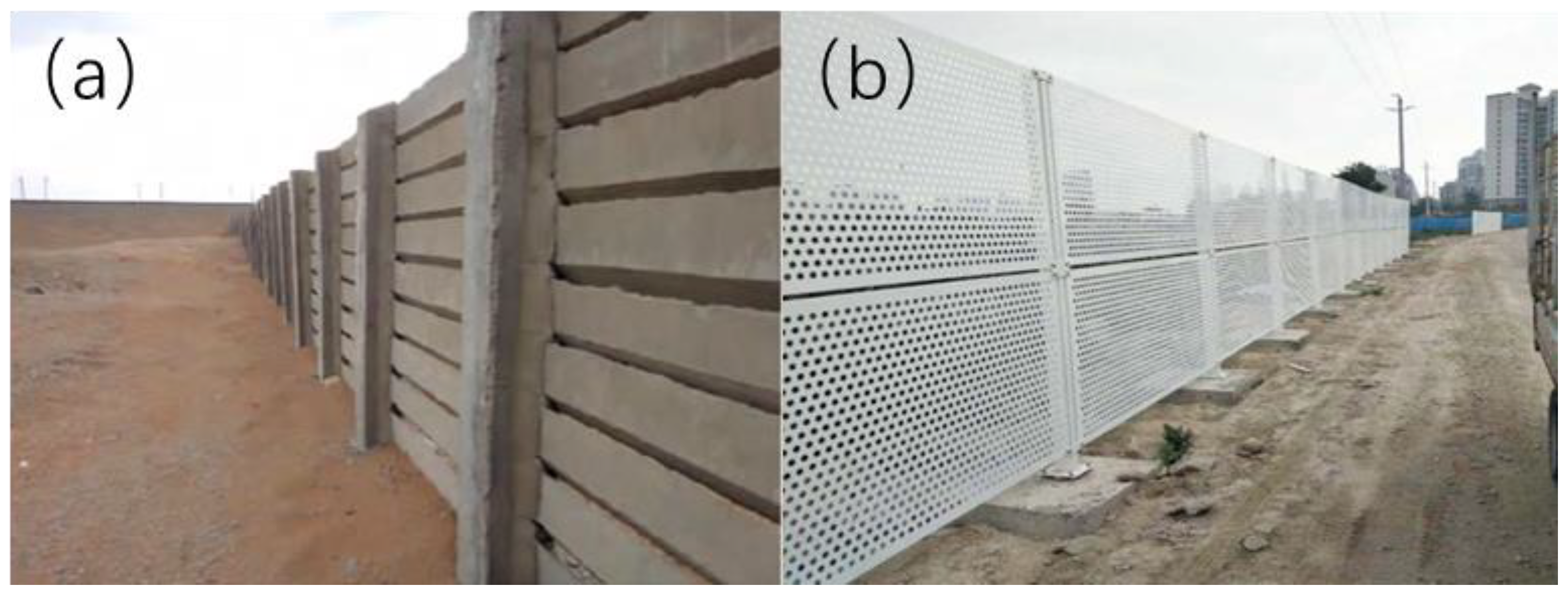
The inclined insert windbreak (
Figure 1a) comprises several inclined panels set at specific angles. Cheng et al. proved through wind tunnel and field tests that the slope insert windbreak has special properties and excellent sand-retarding effects [
6].
Perforated sand fences (
Figure 1b) are the most widely used wind and sand protection structures. Among these, the hole-plate sand fence structure, a new type made of metal plates, stands out due to its excellent durability and reliability. Several factors determine the aerodynamic performance and protection effectiveness of the sand fence, and porosity is the main structure characteristic that affects protection efficiency [
7]. Studies have shown that the optimum porosity of sand fences is 30% [
8]. Perera reported that a porous fence’s porosity influences airflow on the leeward side, and the vortex zone disappears when the porosity exceeds 30% [
9]. They discovered that fences with 30–40% porosity were most effective in reducing mean velocity and surface pressure fluctuations on the leeward side [
10]. Tsukahara et al. used laser sheet visualization to measure the flow field and erosion around a dune, finding that a porosity of 30% most effectively suppressed wind erosion [
11]. The double-row windscreen is the most effective, combining cost efficiency and optimal shielding distance, as numerical simulations and wind tunnel tests demonstrate. Similarly, Fang Hui et al. proposed a cost-effective combination of wind shelter distances using numerical simulations and wind tunnel tests and determined that double-row sand fences were more effective than single-row sand fences [
12]. It is worth noting that along the Qinghai-Tibet Railway, the implementation efficiency of sand fences exceeded 80%. To ensure safe operation and minimize wind and sand damage to tracks, it is essential to enhance the protective performance of wind and sand fences [
13].
It is of great theoretical and practical significance to reduce the disturbance of crosswinds on high-speed railway lines, reduce the deposition of wind sand on rails, and improve its protective effect. This project aims to optimize the design parameters of the new sand fence and evaluate its protective effectiveness by combining wind tunnel tests and numerical calculations [
14]. It is hoped that this will provide reference value to sand prevention and sand control engineering programs along railways and highways.
2. Research Methodology
2.1. Numerical Simulation
2.1.1. Geometric Modeling and Mesh Generation
Given the presence of three-dimensional coupled wind and sand fields in natural environments, theoretically, a larger computational region is better in general. This preference allows for the full development of airflow within the entire area and helps prevent errors caused by eddies and flow detours. However, due to constraints in the working environment, the movement of sand particles is primarily influenced by the airflow’s drag force, resistance, and gravity. Under the influence of the wind field, these forces generally operate within the same plane, thus allowing the problem to be addressed as a two-dimensional issue.
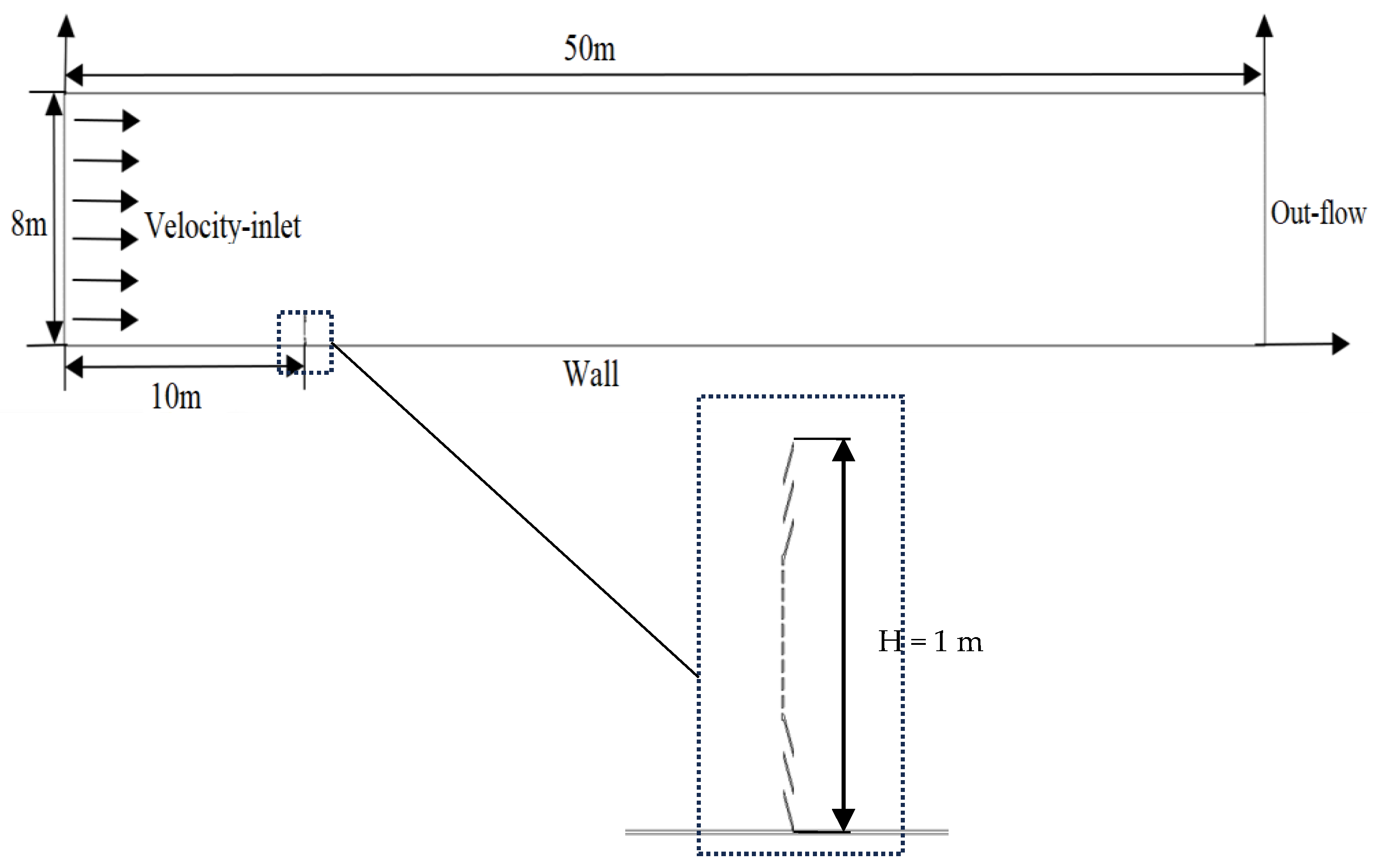
For this study, the dimensions of the computational domain are specified as 50 m in length and 8 m in height, as shown in
Figure 2. The modeled sand fence has a height of 1 m, a thickness of 0.004 m, a pore size of 0.014 m, and a porosity of 0.2. The velocity inlet is 10 m from the sand fence, and the velocity outlet is 40 m from the sand fence.
A well-structured grid division can significantly enhance the simulation process and expedite convergence. Given that this experimental model is a two-dimensional plane model, the mesh is divided into triangular meshes using an unstructured mesh method. To account for the movement characteristics of sand particles on the surface of the wind and sand flow, a sparse top and dense bottom approach is employed for the lower boundary mesh of the model, dividing it layer by layer. Conversely, sparse grids are utilized in regions where the upper fluid exhibits more gradual changes. This strategy not only optimizes the convergence time of the model operation but also ensures the accuracy of the simulation results in key research areas of the experiment, thereby improving both the accuracy and efficiency of the calculations. The total number of grid cells is approximately 450,000, and the grid skewness is less than 0.85, thereby meeting the quality standards for computational grids.
2.1.2. Control Equations
The standard k-ε turbulence model is selected for simulating the net wind field due to its effectiveness in capturing wakes, eddies, and contrails. This model has been extensively employed in previous studies examining airflow around wind fences, yielding results that are consistent with measured values. The Eulerian model is utilized to solve the two-phase flow of wind and sand, incorporating the realizable k-ε turbulence model. Additionally, the SIMPLE algorithm is employed to solve for velocity and pressure [
15,
16,
17].
In this study, the wind-sand flow is simulated using the Eulerian two-fluid model, which primarily involves mass and momentum equations [
18]. The corresponding expressions for these controlling equations are as follows:
Continuity conservation equation:
Momentum conservation equation:
where
ρ is the density (kg·m
−3);
t is the time (s);
,
are the velocity components;
p is the pressure (Pa) on the fluid micro-element body;
is the velocity vector;
,
,
, and
are the components (Pa) of the viscous stress τ acting on the surface of the micro-element body caused by the viscosity of molecules; and g is the acceleration of gravity
To effectively assess the protective performance of the wind fence, the wind protection efficiency is evaluated as follows [
19,
20]:
where
is the sand fence windproof efficiency;
is the distance from the fence and
is the height from the ground (expressed as a multiple of the fence height);
is the wind speed at point (
,
) with the fence protection; and
is the wind speed at point (
,
) under the condition of having no fence protection.
2.1.3. Calculation Parameters
The boundary conditions for the simulation model are as follows: the left side is a velocity-inlet, the right side is an out-flow, and the upper and lower walls are wall boundaries [
21,
22,
23].
Table 1 presents the calculated parameters.
2.2. Wind Tunnel Experiment
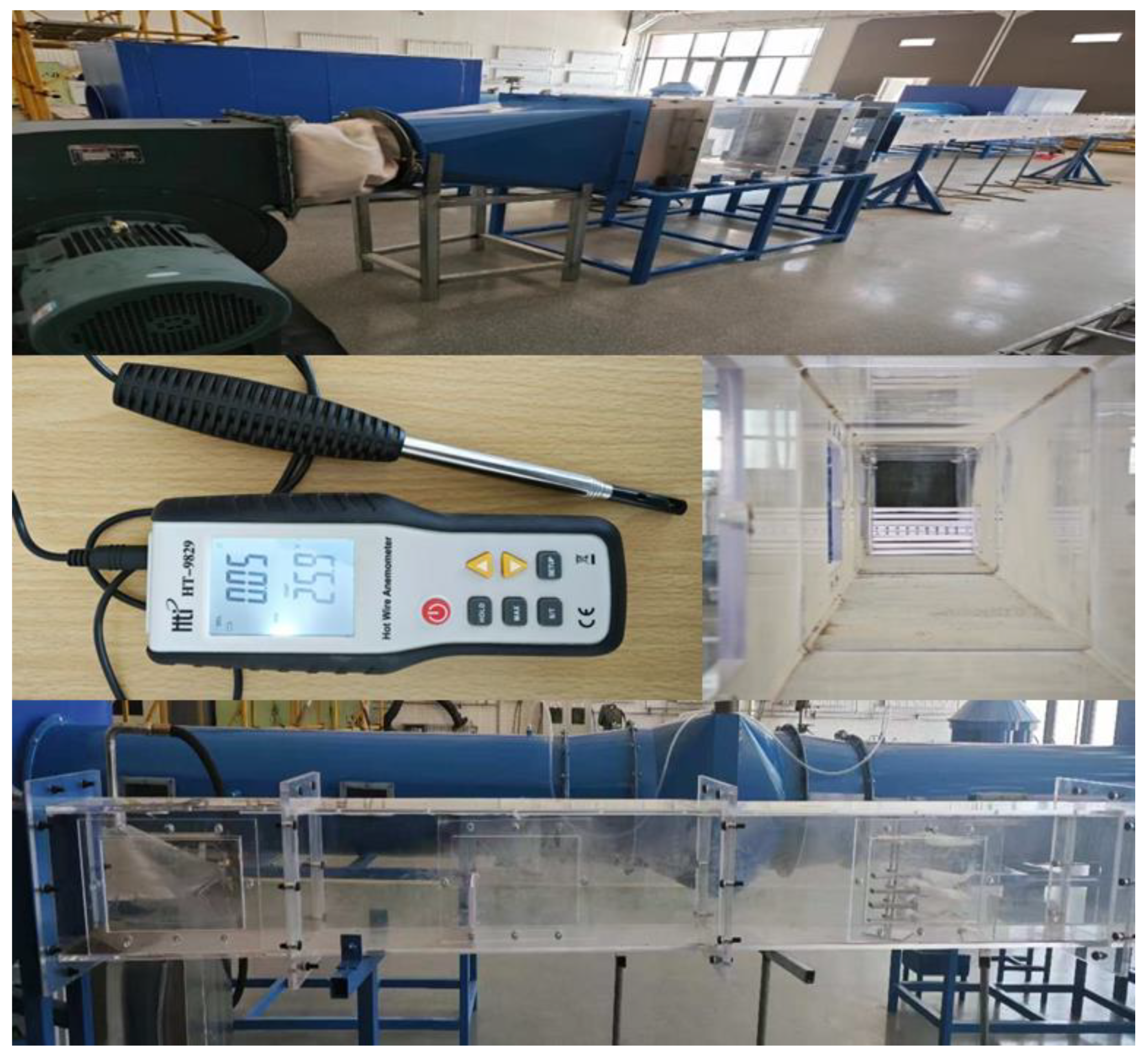
The wind tunnel tests (
Figure 3) discussed in this paper were conducted in the small-scale low-speed DC wind tunnel laboratory at Xinjiang University. The wind tunnel has a total length of 10 m, with a test section measuring 3.5 m. The wind speed within the test section can be continuously adjusted from 0 to 30 m/s. The Reynolds number for the tests ranges from 0 to 1.34 × 10
6, and the turbulence intensity is maintained at less than 1%.
The major goal of the wind tunnel tests is to measure changes in wind speed around the sand fences, with an incoming wind speed of 10 m/s. An anemometer is used to measure wind speeds. These locations are positioned on the windward side at distances of 0.5H, 1H, 1.5H, 2H, 2.5H, 3H, 3.5H, 4H, 4.5H, 5H, 6H, 7H, 8H, 9H, and 10H, where H denotes the height of the sand fence wall. The monitoring points on the leeward side were located at 0.5H, 1H, 1.5H, 2H, 2.5H, 3H, 3.5H, 4H, 4.5H, 5H, 6H, 7H, 8H, 9H, 10H, 11H, 13H, and 15H. To obtain complete data, the wind speeds were examined at 0.8H [
24,
25].
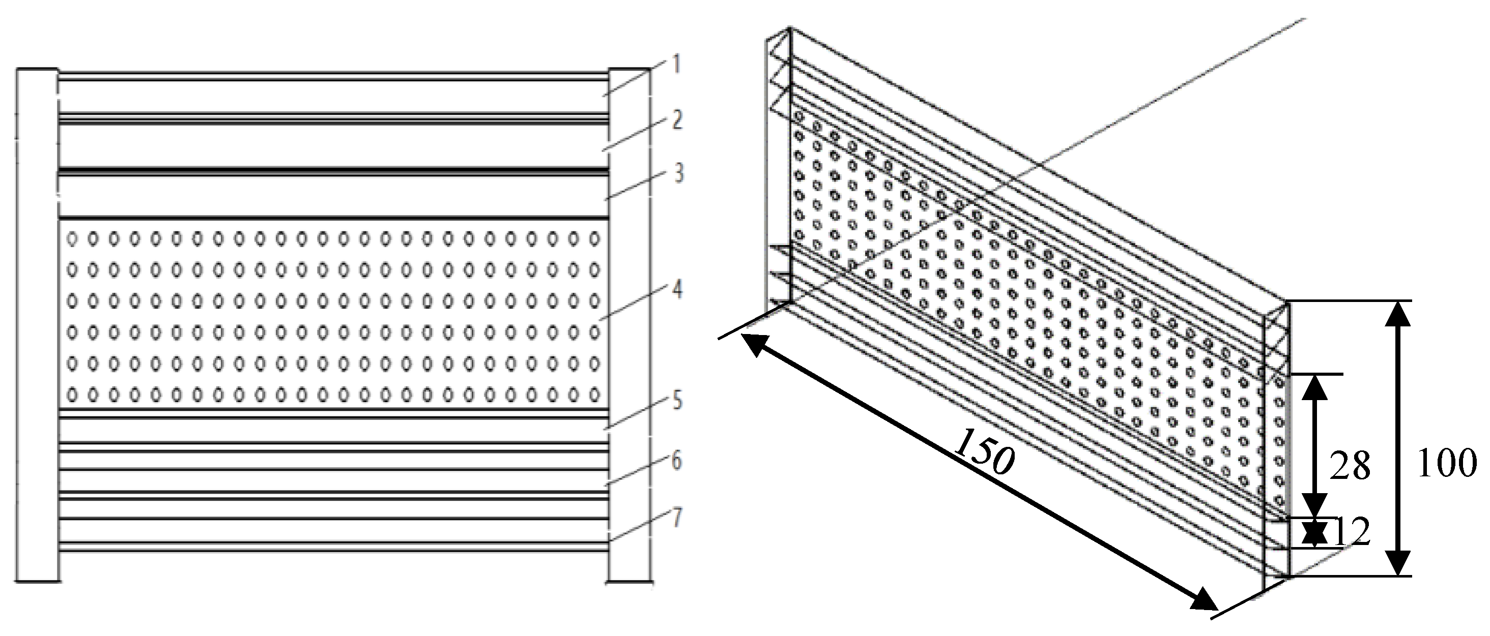
The new sand fence model used in the wind tunnel tests is shown in
Figure 4. This model primarily comprises two columns, six inclined inserts, and one aperture plate. The configuration includes No.1, No.2, and No.3 slanting plates installed in the upper part of the column. In contrast, the No.4 aperture plate, characterized by a 20% porosity, is positioned in the middle part of the column. Additionally, No.5, No.6, and No.7 slanting plates are installed in the lower part of the column. The overall height of the sand fence is 100 mm. The dimensions of the inclined insert plates are 150 mm in length and 12 mm in height, adhering to a model scale of 1:10 [
26]. Meanwhile, the aperture plate measures 150 mm in length and 28 mm in height. The inclined insert and the open plate thickness are 5 mm.
3. Results
3.1. Reliability Verification of Numerical Simulation Results
Numerical simulation offers several advantages, including cost savings in engineering, the ability to obtain comprehensive data, and the efficient optimization of designs. However, their reliability must be reasonably assessed to ensure that these results can scientifically guide engineering practices. A comparison with wind tunnel test results is conducted to verify the reliability of numerical simulation outcomes.
Figure 5 shows the relative wind speed around the sand fence wall obtained from numerical simulations and wind tunnel tests. In this context, H is the height of the sand fence wall, and L is the distance from it, with positive numbers representing the windward side and negative values indicating the leeward side. V
0 refers to the inlet wind speed, V
L is the wind speed at a specific point within the computational domain, and V
0/V
L represents the relative wind speed. The data reveal that the relative wind speed distribution forms an approximate ‘V’ shape as a function of distance. Notably, the patterns in relative wind speed with distance obtained by both methods are essentially consistent, demonstrating the excellent reliability of the numerical simulation results.
Furthermore, the change in relative wind speed can be divided into three parts. Wind speed decreases slightly throughout the initial period (−10H ≤ L ≤ −2H). The second phase occurs when −2H < L ≤ 2H, resulting in a considerable fall in wind speed. During the third phase, when 2H < L ≤ 15H, the wind speed progressively increases. Given that sand particles’ kinetic energy is mostly obtained from wind energy, the observed wind speed trends indicate that sand deposition occurs primarily on the leeward side of the sand fence.
3.2. Characteristics of Air Velocity Changes in a Single-Row Structural Sand Fence
3.2.1. The Effect of Inclined Angle of Single Row Structure Sand Fence on Wind Protection
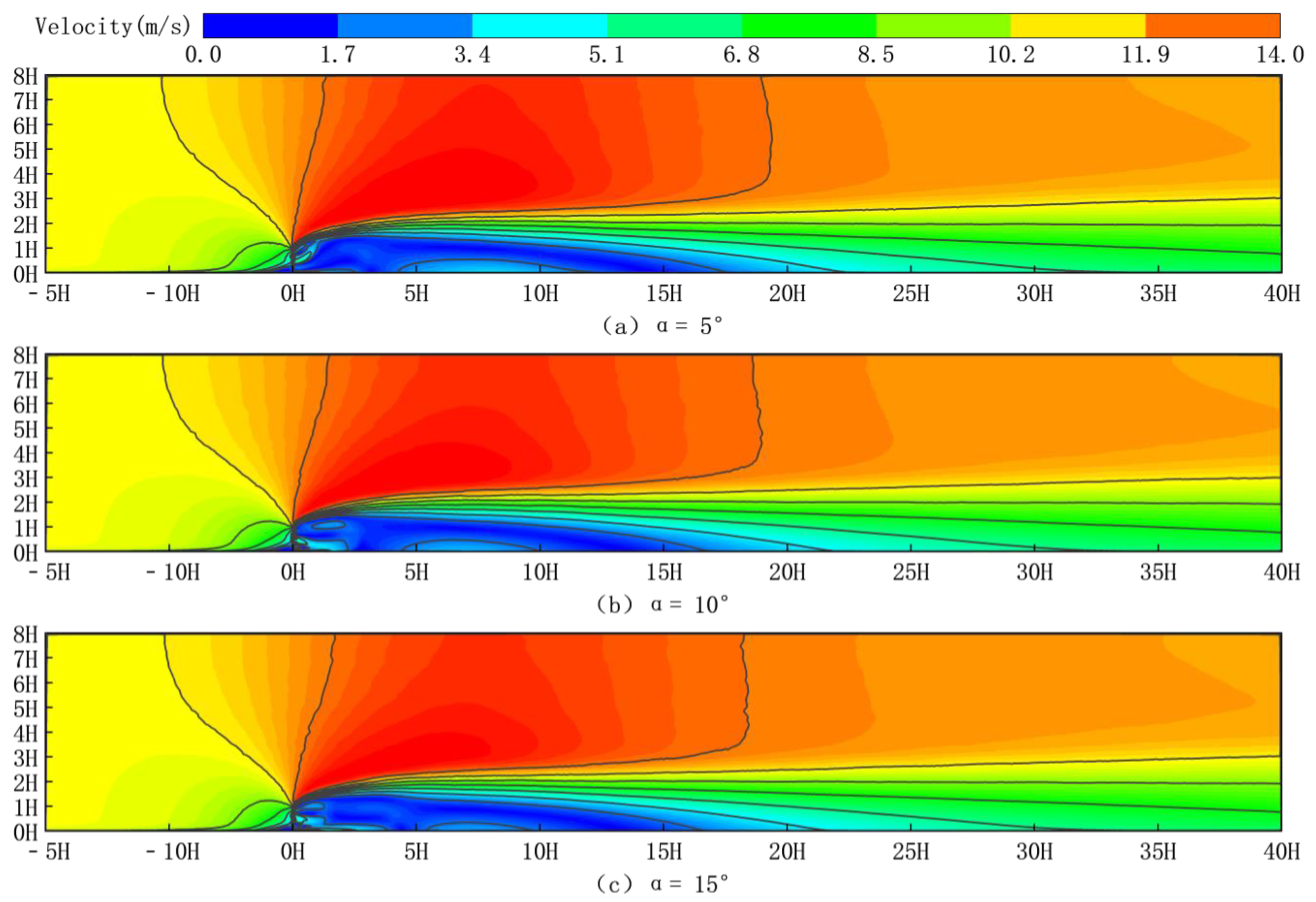
Figure 6 depicts wind speed cloud maps for six different inclined plate angles (angle from vertical) at a wind speed of 10 m/s.
Figure 6a depicts the wind speed cloud map at a 5° tilt angle,
Figure 6b depicts the wind speed cloud map at a 10° tilt angle,
Figure 6c depicts the wind speed cloud map at a 15° tilt angle,
Figure 6d depicts the wind speed cloud map at a 30° tilt angle,
Figure 6e depicts the wind speed cloud map at a 45° tilt angle, and
Figure 6f depicts the wind speed cloud map at a 60° tilt angle.
Figure 6a–f shows that the velocity distribution pattern around the new sand fences is similar to that of existing sand fences, indicating a considerable impact on the airflow structure surrounding them. The sand fences block the approaching airflow, reducing wind speed on the windward side. As a result, deceleration, acceleration, and turbulent zones occur on the windward, top, and leeward sides of the fences, respectively.
Notably, the new sand fences deflect and divert the wind, preventing it from acting directly and vertically on the fences. This causes a minor increase in airflow velocity on the leeward side of the four slanting boards, resulting in a local high-speed zone. These phenomena are principally caused by the lower cross-sectional area of the airflow at the gaps between the slanting boards, which increases the airflow velocity due to the ‘narrow tube effect’. Multiple vortices can be seen around the sand fences, with the leeward side having substantially more and larger vortices than the windward side.
Comparing the different inclination angles in
Figure 6, it can be concluded that sand fences with inclination angles of 5–15° create a larger deceleration zone behind them compared to those with inclination angles of 30–60°. Additionally, the number of vortices generated behind the sand fences with 5–15° inclined inserts is greater than that of the sand fences with 30–60° inclined inserts.
3.2.2. Distribution of Flow Field around the Structure Sand Fence of a Single-Row
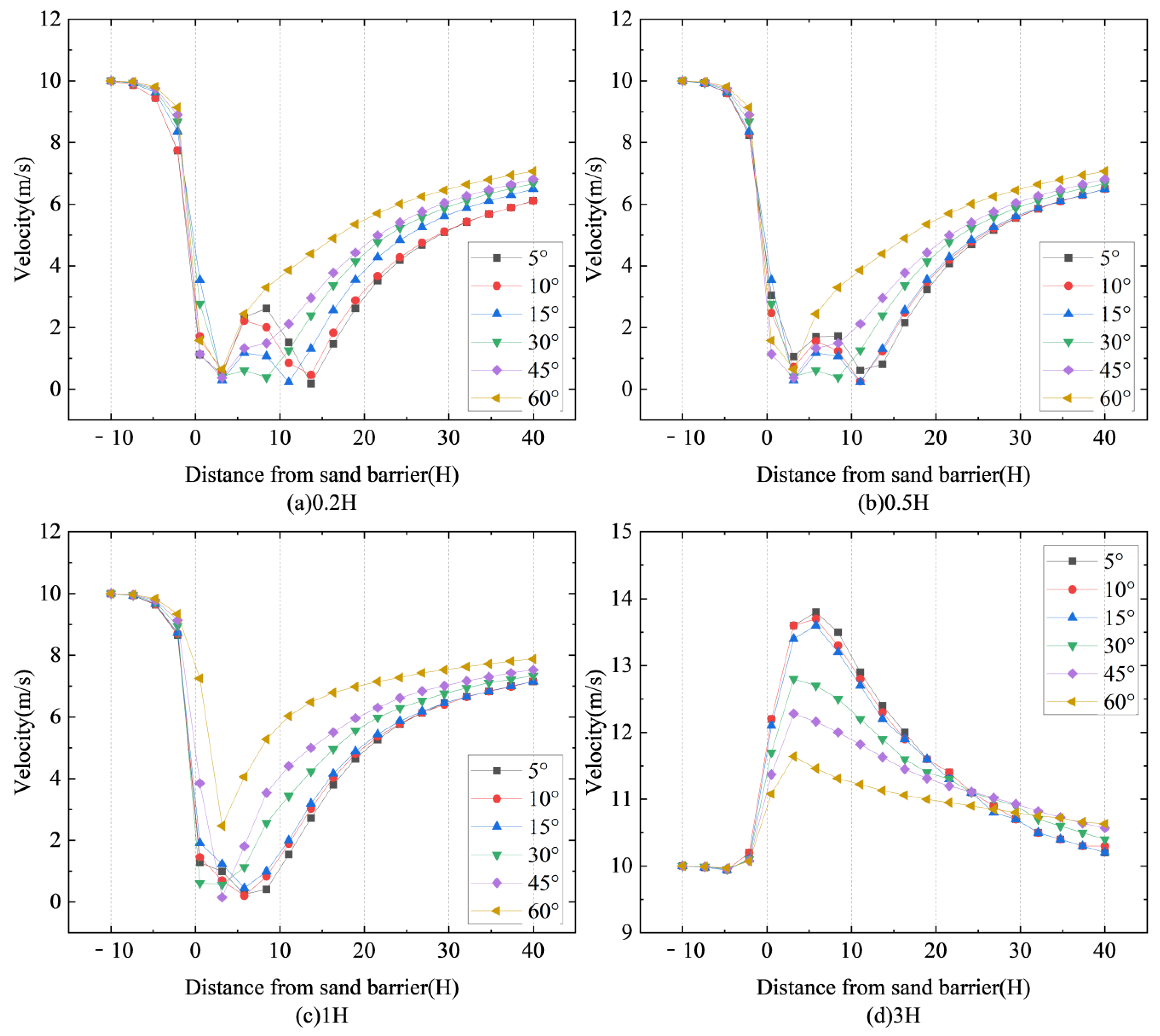
Figure 7 depicts the horizontal wind speed pattern around a novel type of sand fence with different inclination angles of inclined inserts.
Figure 7a depicts the horizontal wind speed at 0.2H above the ground, and
Figure 7b depicts the horizontal wind speed at 0.5H above the ground.
Figure 7c and
Figure 7d depict the horizontal wind speed at 1H and 3H above the ground, respectively.
The sand fences’ overall velocity change curves at heights of 0.2H, 0.5H, and 1H from the ground do not significantly differ from one another. The relative wind speeds exhibit a distribution that approximates a “V” with distance, and the wind speeds generally show a tendency to drop and then increase. Additionally, based on the rate at which the relative wind speeds fluctuate, the relative wind speeds can be loosely split into four categories: the wind speeds marginally drop from −10H to −2H. Wind speeds decrease sharply from −2H to 3H due to the sand fences obstructing airflow, and they reach their lowest value at 3H on the leeward side of the sand fences. From 3H to 6H, wind speeds show a clear upward trend due to the inclination angle of the slanting plate accelerating the airflow on the leeward side. This is because the ramp’s inclination angle accelerates the airflow on the leeward side, and the wind speed progressively recovers between 6H and 40H.
Figure 7d shows that the velocity change of the sand barricade at 3H from the ground is the same as that of the other three heights, and the overall velocity curve shows an inverted ‘V’ shape distribution. This demonstrates that the wind protection impact of the sand fences at the height of 3H is weak, with the main protective range being the height below the sand fence.
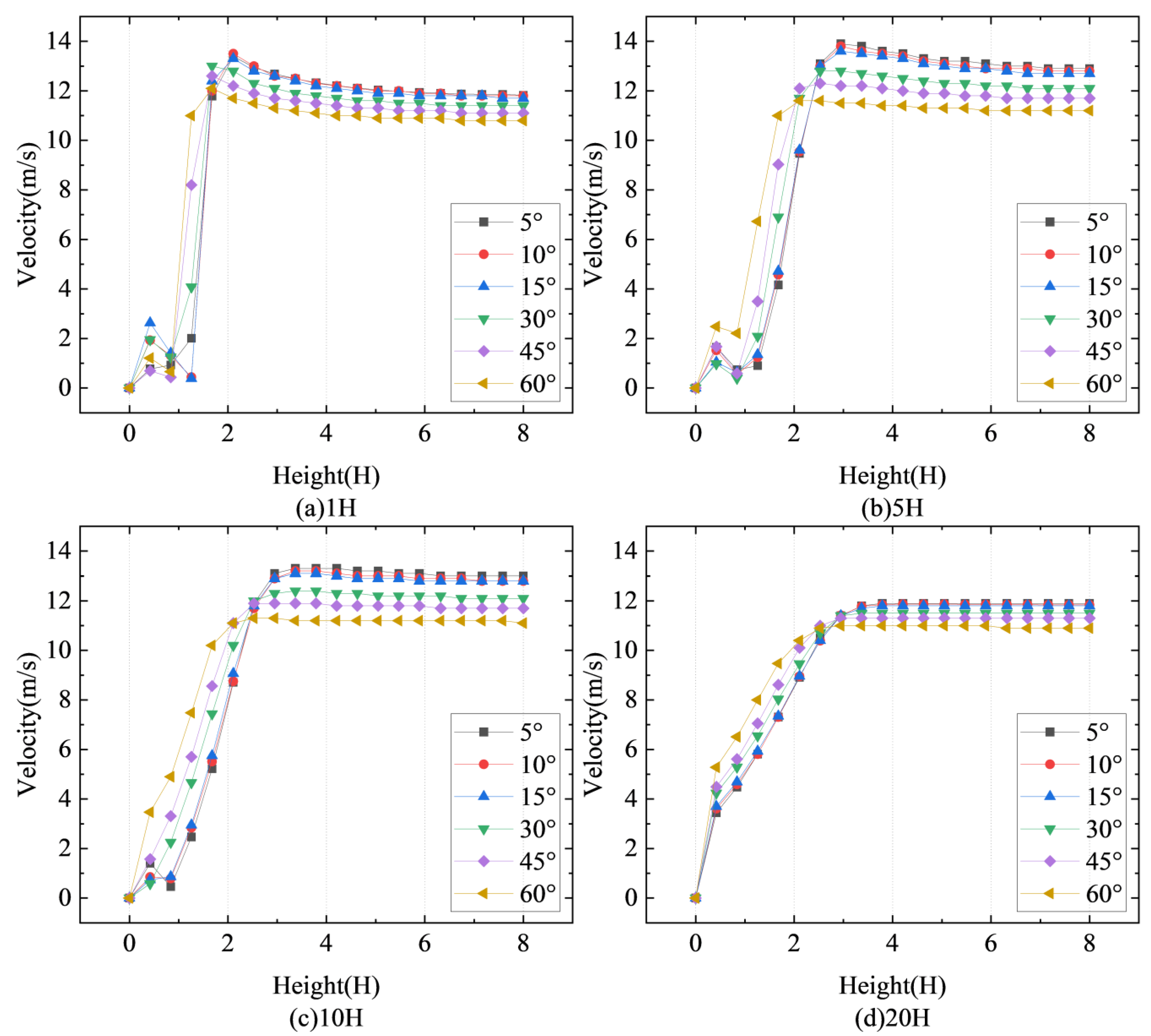
Figure 8 shows the variation in vertical wind speed around the new sand fence at various inclined insertion angles.
Figure 8a displays the vertical wind speed at a distance of 1H from the sand fence, whereas
Figure 8b displays the vertical wind speed at a distance of 5H from the sand fence.
Figure 8c displays the vertical wind speed at a distance of 10H from the sand fence, whereas
Figure 8d displays the vertical wind speed at a distance of 20H from the sand fence.
Wind speed variations at distances of 1H, 5H, 10H, and 20H on the leeward side of the sand fences show modest differences and can be divided into three distinct segments based on height above ground. At heights of ≤1H, wind speed increases and then decreases. Second, at heights between 1H and 2H, the wind speed gradually increases, resulting in an accelerated zone. Finally, as the height above the ground surpasses 2H, the sand fences’ acceleration impact lessens, resulting in a progressive stabilization of wind speed due to contact with low-speed external airflow.
3.2.3. The Variation of the Effective Protection Range of a Single-Row Structure Sand Fence
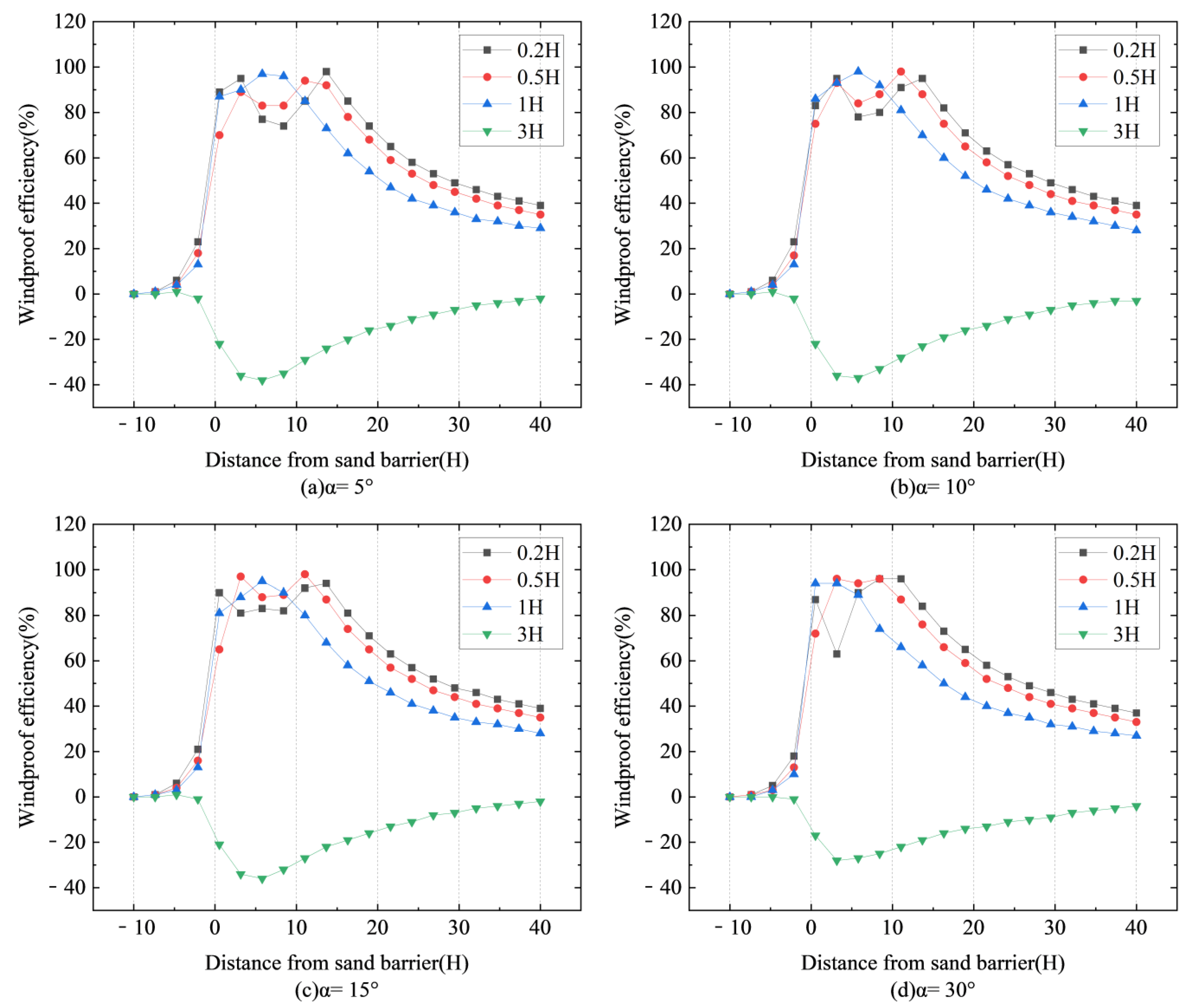
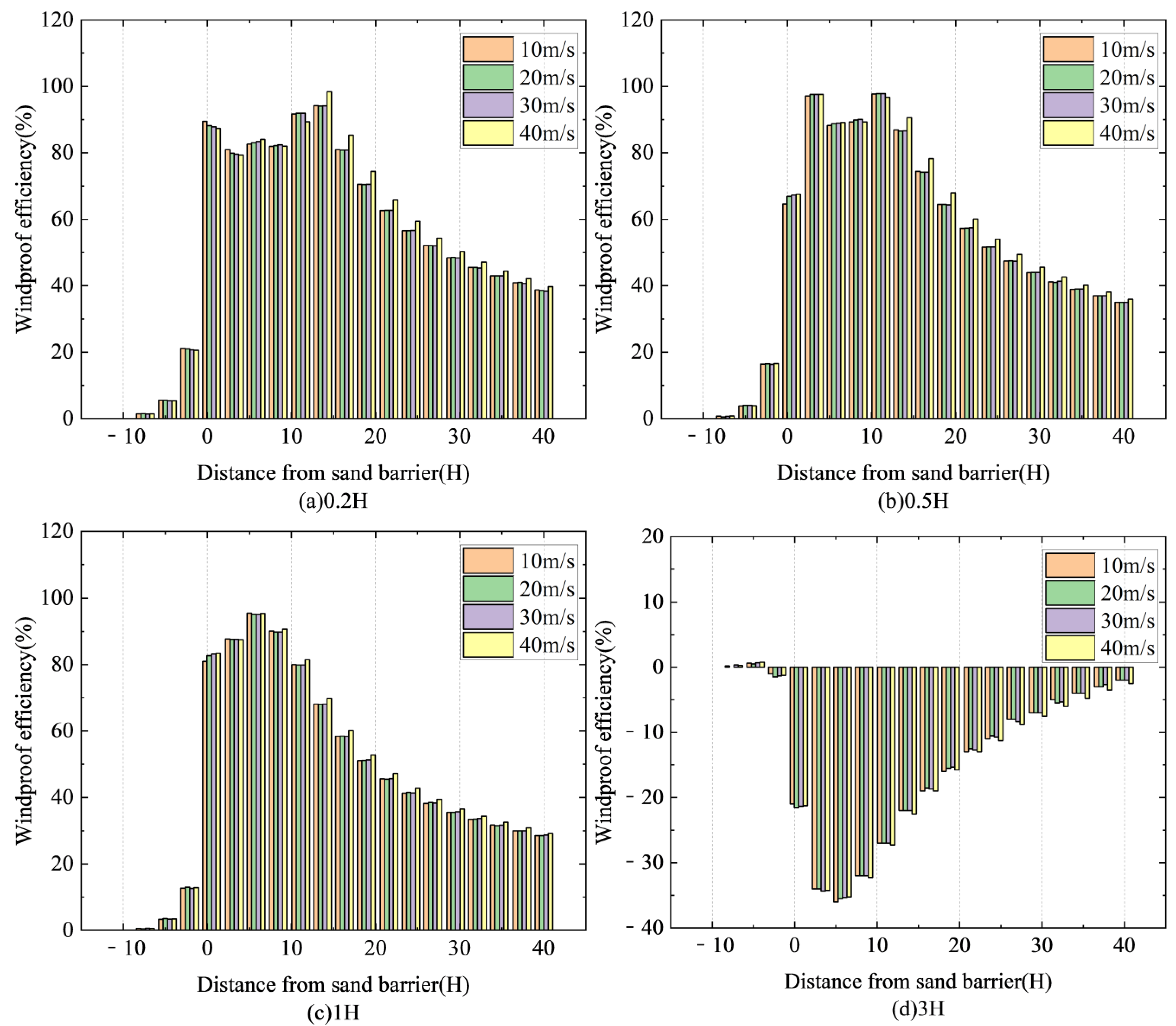
Figure 9 selects four heights of 0.2H, 0.5H, 1H, and 3H, and calculates the windproof efficiency of six different inclined sand fences according to Formula (4).
Figure 9a shows the windproof efficiency at a tilt angle of 5°;
Figure 9b shows the windproof efficiency at a tilt angle of 10°;
Figure 9c shows the windproof efficiency at a tilt angle of 15°; and
Figure 9d shows the windproof efficiency at a tilt angle of 30°.
Figure 9 illustrates the wind protection efficiency of sand fences at six different inclination angles under a wind speed of 10 m/s. The data reveal distinct upward and downward trends, with the overall pattern resembling an ‘M’ shape. Notably, when the height from the ground reaches 3H, the protection efficiency of all sand fences becomes negative.
Figure 9c shows that when the inclined insertion plate has an inclination angle of 15°, the windproof efficiency change curve in the range of 0H to 11H is the smoothest, and the windproof efficiency is greater than 80% at heights of 0.2H, 0.5H, and 1H above the ground. This suggests that the protection of the new sand fencing is mainly near the ground level. When the inclination angle of the inclined baffle is 15°, the windproof efficacy of the leeward side of the sand fence is optimal, and the longest effective protection distance supplied is 11 m. Therefore, 15° is the optimal inclination angle for the inclined insertion plate.
3.2.4. Distribution of Flow Field around a Single-Row Structure with Different Air Velocities
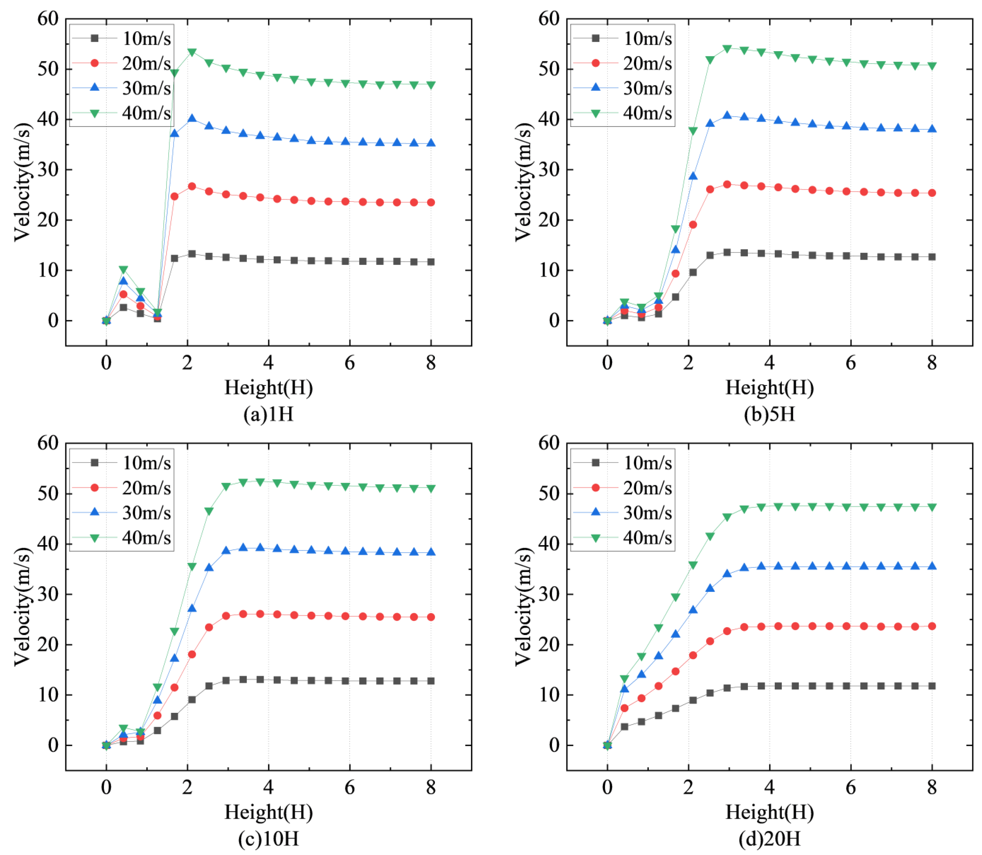
Figure 10 depicts the differences in horizontal wind speed at various heights surrounding the sand fence for wind speeds of 10 m/s, 20 m/s, 30 m/s, and 40 m/s.
Figure 10a shows the horizontal wind speed at an altitude of 0.2H, whereas
Figure 10b shows the horizontal wind speed at an altitude of 0.5H.
Figure 10c and
Figure 10d show the horizontal wind speed at 1H and 3H altitudes, respectively.
From
Figure 10a–c, it is evident that the wind speed trends at different heights exhibit a consistent pattern under four distinct wind speed conditions, approximately resembling a “W” shape. Upon encountering a sand fence, the wind speed experiences a sharp decrease, followed by a gentle zone in the wind speed variation lines. Within this gentle zone, the wind speed reaches its minimum value, and the variation lines for the four wind speed conditions converge and eventually overlap. This convergence indicates that the magnitude of the wind speed has minimal impact on the wind speed characteristics within a small distance around the sand fence.
From
Figure 10d, it can be seen that throughout the entire flow field, the wind speed variation remains at 40 m/s at the top, followed by 30 m/s, then 20 m/s, and finally 10 m/s, indicating that the magnitude of wind speed will have an impact on the wind speed characteristics at high positions on the leeward side of the new sand fence.
Figure 11 depicts the vertical fluctuation in wind speed around the sand fence under various wind conditions.
Figure 11a shows the vertical wind speed at a distance of 1H from the sand fence, whereas
Figure 11b shows the vertical wind speed at a distance of 5H.
Figure 11c depicts the vertical wind speed at a distance of 10H, whereas
Figure 11d displays the vertical wind speed at a distance of 20H from the sand fence.
Upon analyzing
Figure 11, a consistent air speed change trend can be observed at the positions of 1H, 5H, and 10H behind the sand fence. At heights ranging from 0H to 0.2H above the ground, there is a notable sharp increase in all four wind speeds as height increases. Subsequently, within the height interval from 0.2H to 1.2H above the ground, the air speed demonstrates a gradual decrease, eventually converging. At a distance of 20H behind the sand fence, the air speed initially exhibits a linear increase, followed by a curved pattern. As the height increases to between 1.2H and 2.1H above the ground, there is a rapid rise in air speed variations, resulting in a peak value that exceeds the initial air speed. Air speed then slightly decreases towards the initial air speed when the height exceeds 2.1H above the ground. The study affirms that air speed has a minimal impact on the flow field characteristics near the ground of the newly implemented sand fence.
Figure 12 shows the windproof effectiveness of sand fences at various wind speeds.
Figure 12a shows the windproof efficiency at 0.2H above ground, while
Figure 12b shows the efficiency at 0.5H.
Figure 12c depicts windproof efficiency at a height of 1H above the ground, while
Figure 12d displays efficiency at a height of 3H.
Figure 12 illustrates the windproof efficiency of the new sand fence at various heights above the ground under different wind speeds. At heights of 0.2H and 0.5H, the windproof efficiency remains relatively stable, suggesting that within a certain range of wind speeds, the sand fence’s performance is unaffected. However, at a height of 1H, there is a noticeable reduction in windproof efficiency, and at 3H, the sand fence exhibits almost no windproof effect. These observations indicate that while excessive wind speed does not significantly alter the flow characteristics of the sand fence near the ground, its effectiveness diminishes with increasing height. Consequently, this new type of sand fence is well-suited for high wind speed environments, providing a viable solution to mitigate issues such as train shutdowns or overturning caused by strong winds in northwest China.
3.2.5. Sand Accumulation Characteristics of a Single-Row Structure Sand Fence
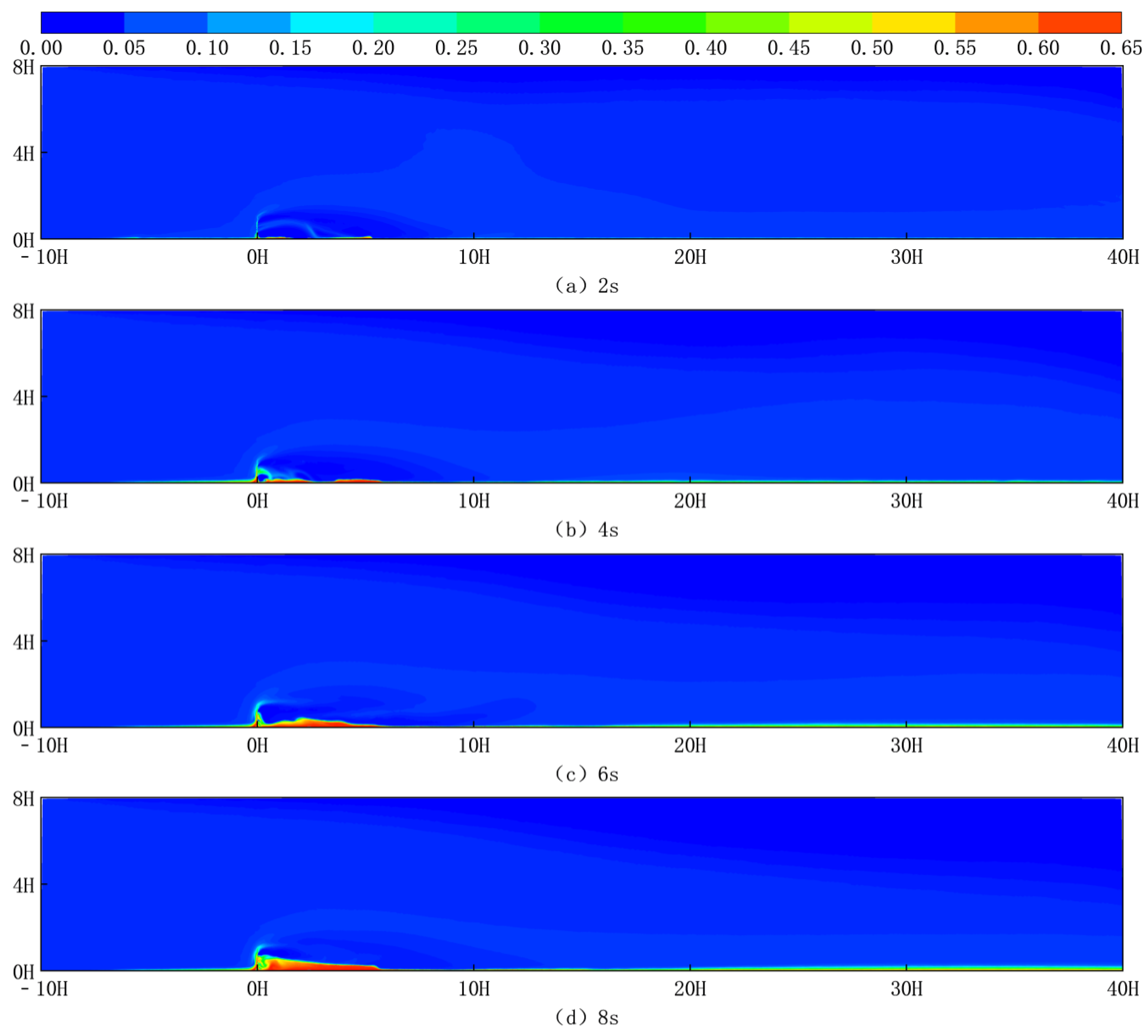
Figure 13 shows the sand cloud at different moments at 10 m/s for the new sand fences with 15H spacing.
Figure 13a depicts the collected sand cloud at 2 s,
Figure 13b depicts the accumulated sand cloud at 4 s,
Figure 13c depicts the accumulated sand cloud at 6 s, and
Figure 13d represents the accumulated sand cloud at 8 s. As shown in the diagram, when sand-laden wind enters the flow field area through the left velocity intake, it hits a new sand fence. This interaction reduces wind speed, resulting in a decrease in sand-carrying capacity. As a result, sand particles begin to deposit mostly on the leeward side of the sand fence, albeit some accumulate on the windward side.
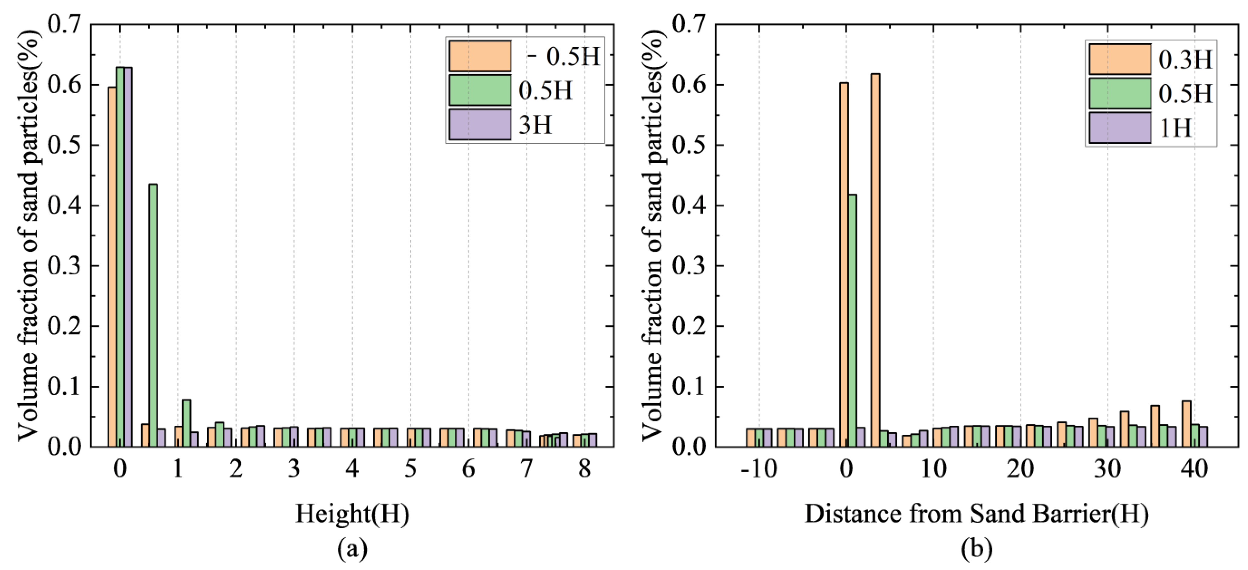
Figure 14 depicts a bar chart of the volume fraction variations of sand particles at various locations along the sand fence over 8 s. The wind speed carrying sand is 10 m/s, and the sand particles have an initial volume fraction of 3%.
Figure 14a depicts the volume percentage of sand particles at different heights relative to the first row of sand fences, namely −0.5H, 0.5H, and 3H. The statistics show that when the height is less than 1H, the volume fraction of sand particles in all three positions is much larger than when the height exceeds 1H. This pattern reveals a significant drop in the volume fraction of sand particles as height increases. It shows that the sand fences cannot effectively intercept sand particles above the height of the fences.
Figure 14b depicts the volume percent of sand particles at different horizontal positions relative to the sand fence, with heights of 0.3H, 0.5H, and 1H. As shown in the figure, within 5H of the sand fence, the volume percentage of sand particles is much larger at heights of 0.3H and 0.5H than at other locations. This observation shows that the principal sedimentation location for sand particles is located behind the sand fence.
3.3. Characteristics of Airflow Velocity Variation in Double-Row Sand Fences
3.3.1. The Influence of Different Spacing of Double-Row Sand Fences on Windbreak Effect
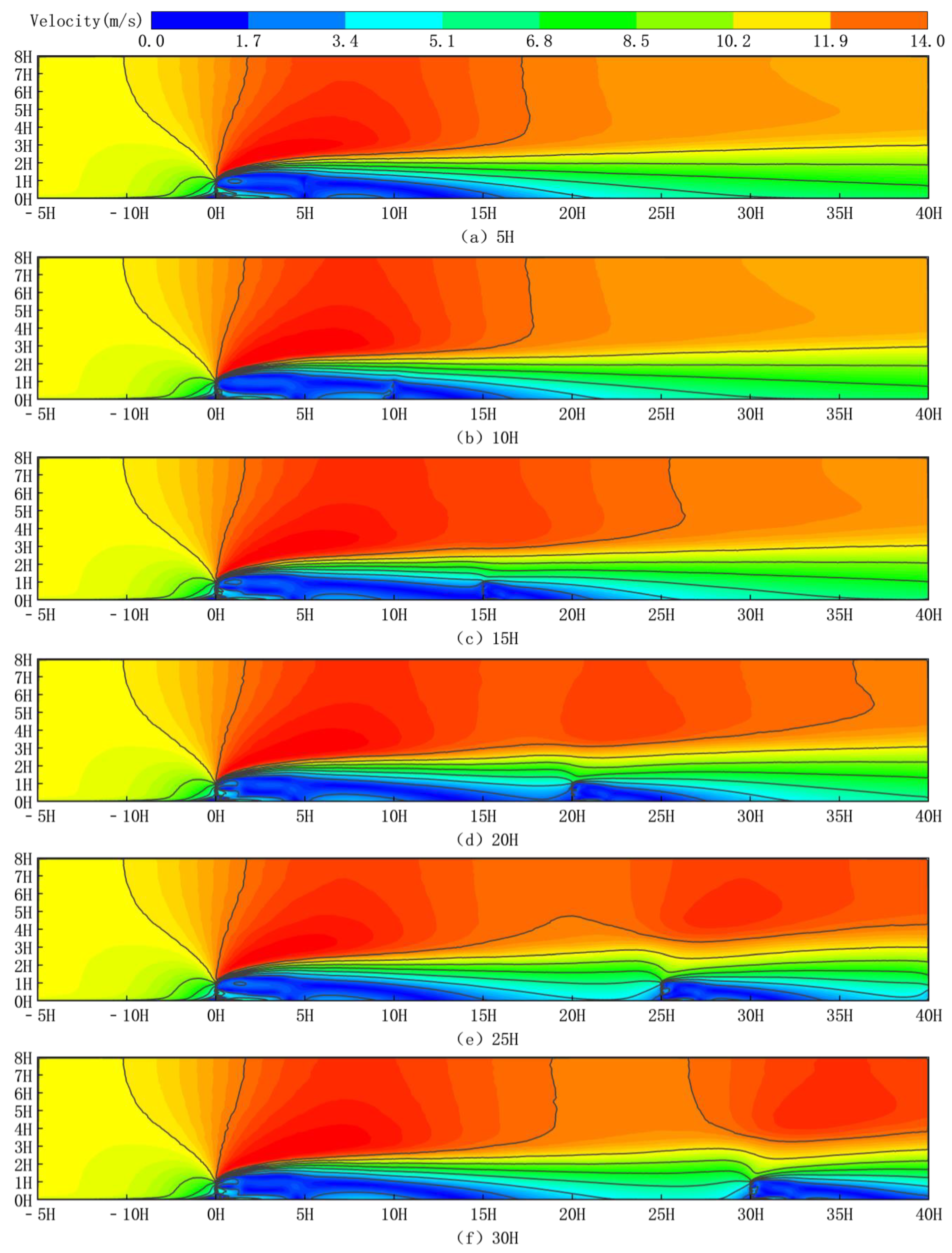
Figure 15 depicts wind speed cloud maps for six configurations of double-row sand fences, each with a different spacing, at a wind speed of 10 m/s. Specifically,
Figure 15a illustrates the wind speed distribution for a double-row spacing of 5H, while
Figure 15b depicts a scenario with a spacing of 10H. Similarly,
Figure 15c shows the wind speed cloud map for a spacing of 15H, and
Figure 15d represents the configuration with a 20H spacing. Furthermore,
Figure 15e and
Figure 15f display the wind speed distributions for spacings of 25H and 30H, respectively.
From
Figure 15, it can be seen that there are deceleration zones in front of the sand fences, acceleration zones above the sand fences, and vortex zones in the middle and behind the two rows of sand fences around the six different spacing sand fences. When airflow reaches a sand fence, its velocity varies dramatically, and a deceleration zone forms on the sand fence’s windward side as a result of the fence. Because the majority of the airflow travels upward when it reaches the top of the sand fence, a concentrated and continuously accelerating airflow produces an airflow acceleration zone above the sand fence. The airflow is accelerated by passing through the slanted insert gaps of the new sand fences. When the accelerated airflow reaches the second row of sand fences, it accelerates again.
The upper layer airflow on the windward side of the first sand fence progressively increases, and a turning point of airflow change develops near the −2H position, forming a weak wind zone. Above the sand fence, a strong wind zone forms, and a vortex forms on the leeward side. The distance between the two sand fences causes changes in the locations and protection ranges of strong and weak winds.
The overall trend is that as the distance between the two rows of sand fences increases, the windward airflow rises slowly, and the number of vortices emerging behind the sand fences progressively increases. The airflow in the transition zone of the double-row sand fences is steady and eventually shortens. When the airflow reaches the second row of sand fences, the recovery distance steadily increases, revealing a “bimodal” airflow fluctuation pattern macroscopically.
3.3.2. Distribution of Flow Field around the Double-Row Sand Fence
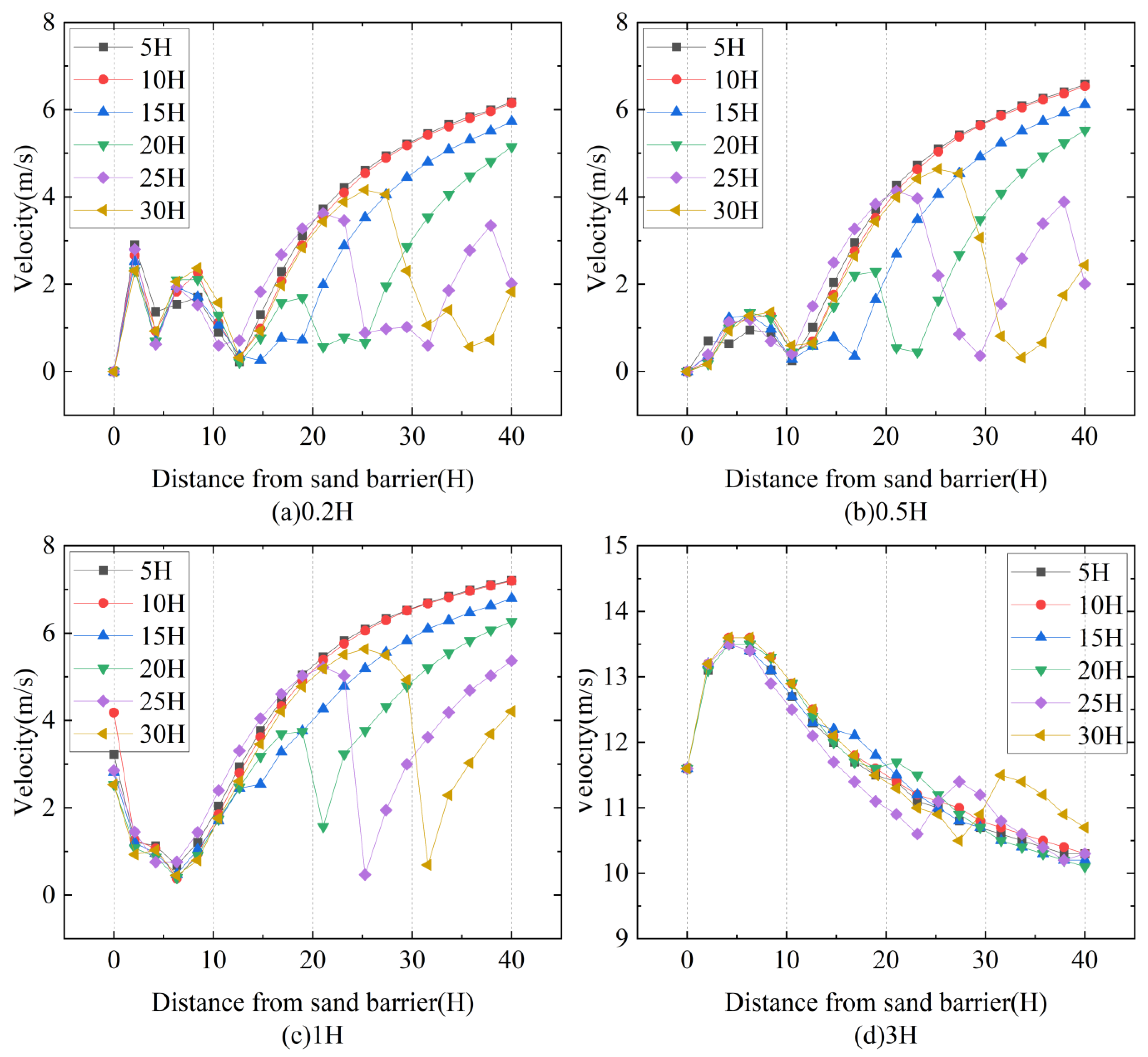
Figure 16 depicts the horizontal fluctuation in wind speed at various heights on the leeward side of a double-row sand fence, starting with a wind speed of 10 m/s.
Figure 16a shows the horizontal wind speed at a height of 0.2H, whereas
Figure 16b shows the wind speed at 0.5H.
Figure 16c and
Figure 16d show the horizontal wind speed at 1H and 3H, respectively.
Figure 16 shows that wind speed fluctuations on the leeward side of the six types of double-row sand fences follow an “N”-shaped pattern. As the distance from the sand fence increases, so does the wind speed, suggesting that the sand fence’s windproof effect is gradually weakened. Finally, the wind speed recovers to its original value, indicating the sand fence’s declining influence over distance. Sand fences with a double-row spacing of 20H had a significantly smoother wind speed change than other sand fences, and it took longer for wind speed to recover to the starting wind speed.
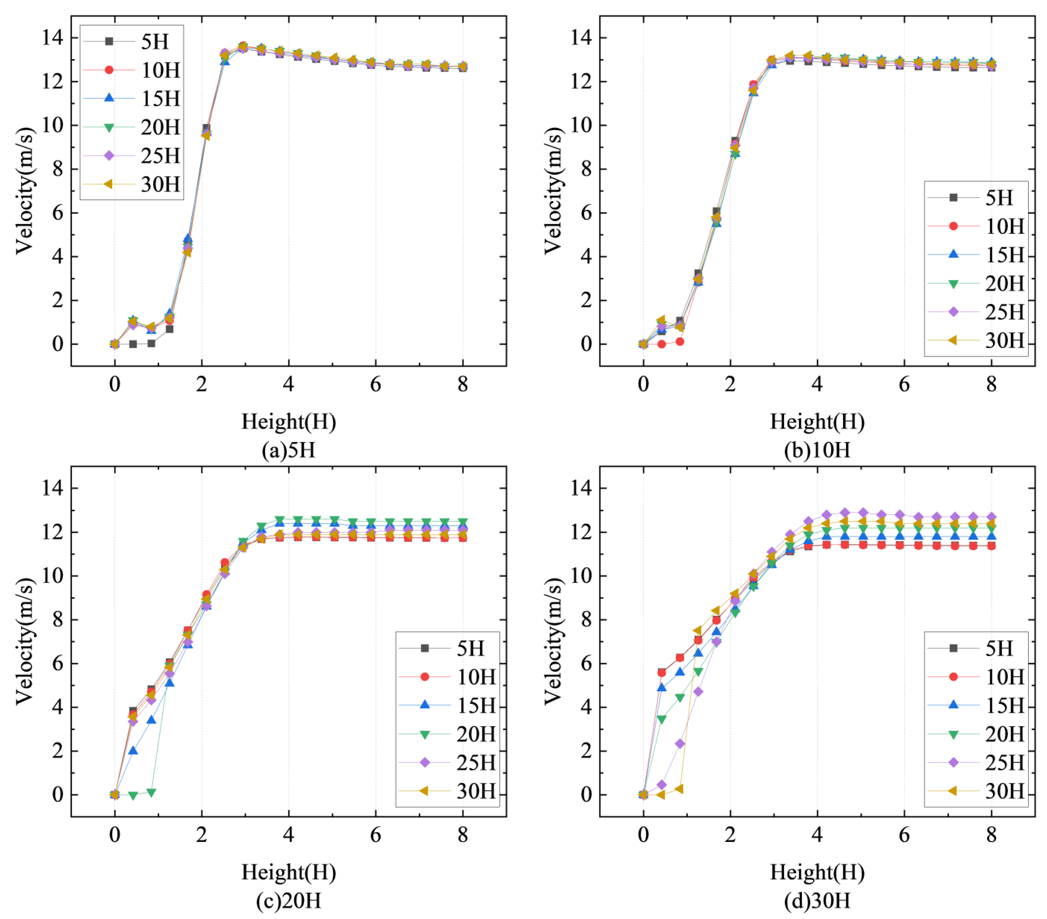
Figure 17 depicts the trend of vertical wind speed variation at several places relative to the double-row sand fence.
Figure 17a depicts the vertical wind speed at a distance of 5H from the first sand fence, and
Figure 17b depicts the vertical wind speed at a distance of 10H from the first sand fence. Furthermore,
Figure 17c depicts the vertical wind speed at a distance of 15H from the first sand fence, whereas
Figure 17d depicts the vertical wind speed at a distance of 20H from the first sand fence.
All six of the sand fences with different spacing provided good surface speed reduction, and the wind speeds were significantly lower than the initial wind speeds up to the 0–1H height, which indicates that the fences provide good wind protection near the surface, and the further the distance from the first row of fences, the less effective the wind protection near the surface becomes.
3.3.3. Changes in the Effective Protection Range of Double-Row Sand Fences
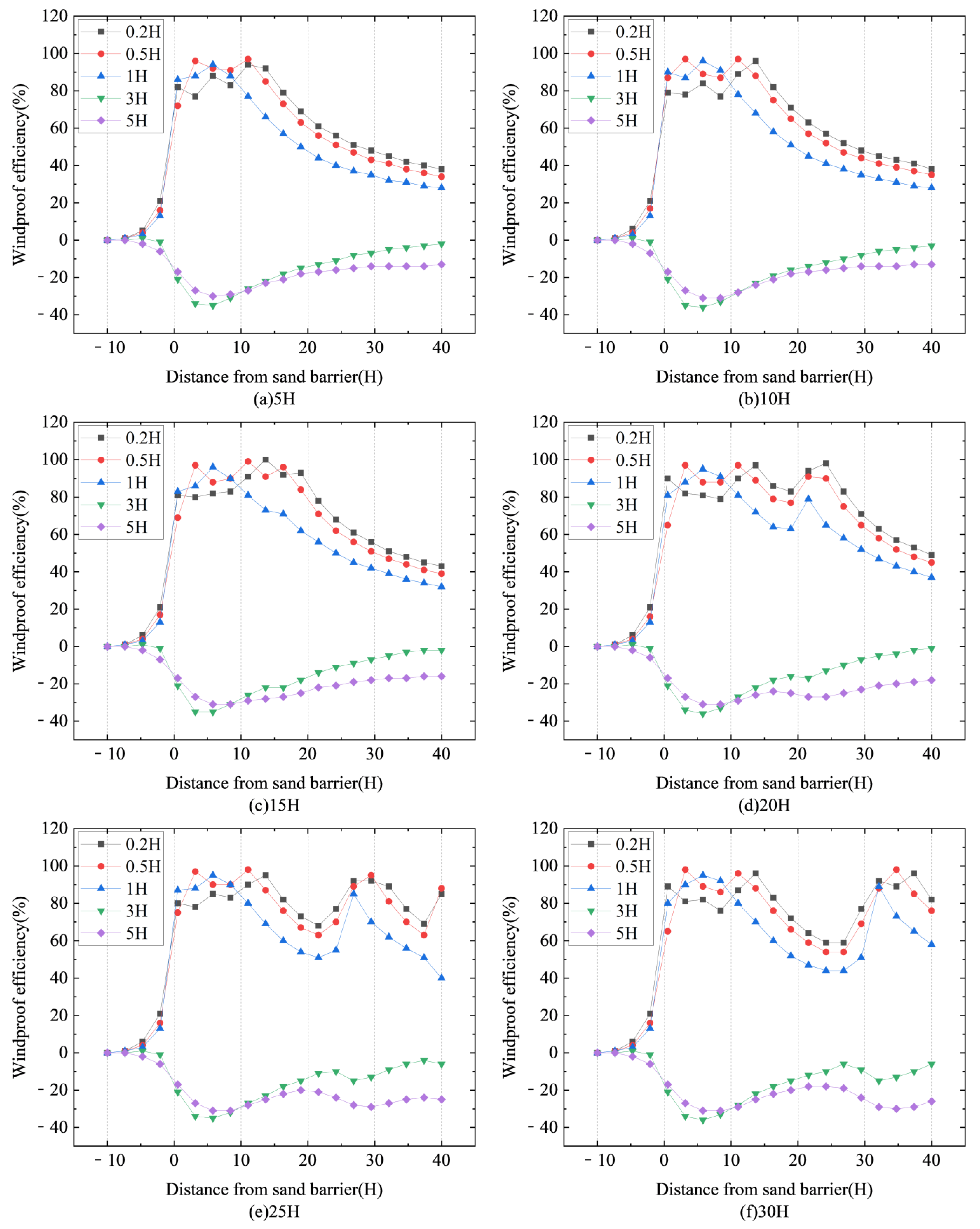
Figure 18 illustrates the windproof efficiency of six different spacing configurations for double-row sand fences, calculated using Formula (4). Specifically,
Figure 18a illustrates the efficiency for a spacing of 5H. Similarly,
Figure 18b depicts the windproof efficiency for a spacing of 10H, while
Figure 18c shows the efficiency for a spacing of 15H. Furthermore,
Figure 18d demonstrates the windproof efficiency for a spacing of 20H, and
Figure 18e illustrates the efficiency for a spacing of 25H. Finally,
Figure 18f illustrates the efficiency for a spacing of 30H.
Figure 18 depicts the windproof performance of six varied spacing double-row sand fences at a wind speed of 10 m/s. The data show distinct upward and downward trends, exhibiting overall uniformity in the patterns.
From
Figure 18a–c, it can be seen that the overall trend of windproof efficiency of sand fences with double-row spacing of 5H, 10H, and 15H is consistent, with a transition zone where the windproof performance first increases, then stabilizes, and finally decreases with distance. Within the range of −10H to 0H, the windproof performance of sand fences gradually increases; within a distance of 1H to 3H, the sand fence reaches its maximum windproof performance. Wind-proof performance increases rapidly in the transition zone between 5H and 9H of the double-row sand fence before gradually decreasing. Similarly, on the leeward side of the second row of sand fences, windproof performance exhibits an initial boost, followed by a gradual fall. Furthermore, the wind fence’s effective protection distance, defined as having a windproof performance of more than 80% at a height of 1H, gradually improves as the distance between the double-row sand fences increases.
From
Figure 18d–f, it can be seen that there are two distinct transition zones in the sand fences with double row spacing of 20H, 25H, and 30H. This is because the longest protection distance of a single-row sand fence is limited. When the spacing exceeds the longest protection distance of a single-row sand fence, the overall wind resistance performance first increases and then stabilizes with the distance, then decreases and slowly rises to a plateau, and finally slowly decreases. Within the range of −10H to 0H, the windproof performance of sand fences gradually increases; within a distance of 1H to 3H, the sand fence reaches its maximum windproof performance for the first time; within the transition zone of 5H to 9H in the double row sand fence, the windproof performance rapidly increases and then slowly decreases; and after the appearance of the second sand fence, the windproof performance rises again and returns to the transition zone, and finally slowly declines.
At heights of 3H and 5H, the windproof efficiency of six variously spaced double-row sand fences is consistently less than 0. This negative windproof effect is due to the influence of the acceleration zone, which suggests that the sand fences have little effect on lowering the kinetic energy of the airflow at these heights, resulting in poor protection performance. The effective protection height of visible sand fences is approximately 1H. Among the configurations tested, a double-row sand fence with a spacing of 20H has the highest windproof efficiency and the longest effective protection distance. Therefore, a spacing of 20H is the optimal spacing.
4. Discussion
This article focuses on two factors: the inclination angle of the inclined insertion plate of the sand fence and the distance between the sand fences, examining their effects on wind protection efficiency and sand accumulation.
After numerically simulating a novel form of sand fence with various inclination angles of inclined inserts, it was discovered that when airflow passes through the sand fence, the horizontal wind speed profile takes on a “V” shape. The overall changes in the horizontal flow field show that when airflow passes through a sand fence system, the closer the windward side of the surface airflow is to the sand fence, the greater the weakening influence on wind speed. The sand fence disturbs the bottom airflow, resulting in a range of weak or quiet wind zones on the leeward side. The inclination angle of the inclined baffle has a considerable impact on the protective effect of sand fences, and this protective effect improves as the inclination angle increases. When the inclined baffle’s inclination angle exceeds 15°, the protective effect begins to diminish.
In terms of sand accumulation, as in the case of flow field characteristics, the new sand fences with different inclinations of the inclined inserts settle sand particles on the leeward side and within the sand fence deceleration zone. Sand fences cannot intercept sand particles above their height.
Because a single-row sand fence has a limited protection range, simulating the protective effect of a double-row sand fence revealed that the effectiveness of a double-row sand fence is superior to that of a single-row sand fence, which can effectively reduce wind speed and better control sand particle movement. When the protective effects of double-row sand fences with varying spacing are compared, it is clear that the protective effect is proportional to the spacing. When the spacing exceeds 20H, the protective effect is reduced.
Many factors affect the effectiveness of the new type of inclined insertion opening combination mechanical sand fence protection, such as sand fence porosity, height, spacing, number of rows, layout form, and natural environmental conditions. Therefore, only a few limiting factors were selected in this study, and it was found that when the inclination angle of the sand fence’s oblique insertion plate is 15° and the double-row spacing is 20H, the sand fence can achieve a higher protective effect.
5. Conclusions
Aiming at the shortcomings of traditional sand fences, a new type of inclined insertion hole combination mechanical sand fence is proposed, and its sand prevention performance is analyzed by combining wind tunnel tests and numerical simulations. At the same time, the design parameters of the inclined insertion plate’s inclination angle and double-row spacing are optimized, and the following conclusions are drawn.
- (1)
Given the differences between inclined wind fences and perforated sand fences, it is clear that each has specific advantages in minimizing the effects of wind and sand on high-speed trains. The inclined wind fence, affected by the “narrow tube effect”, creates a localized high-speed airflow zone on the leeward side of the inclined plate, preventing sand particles from settling on the track. On the other hand, the perforated sand fence effectively obstructs the intrusion of crosswinds. By integrating these two structures, the combined system enhances overall practicality and effectiveness compared to using a single sand fence alone.
- (2)
The inclined insertion plate’s angle relative to the vertical direction determines the new mechanical sand fence’s defensive effectiveness. The protective function of the sand fence increases as the angle of the sloped installation plate increases. When the inclination angle of the inclined insertion plate is 15°, the protective performance is ideal, and the protective effect declines as the angle exceeds 15°.
- (3)
The gap between double-row sand fences affects their protective function. The defensive efficacy of sand fences improves as the distance between two rows increases. When the distance between the two rows of sand fences is 25H, the protective performance is optimal. The protective performance reduces as the distance exceeds 25H.
- (4)
The effective protection height of the new mechanical sand fence corresponds directly to its physical height, as it is incapable of intercepting sand particles that exceed this height. Furthermore, the credibility of the numerical simulations is reinforced by their consistency with wind tunnel test results, particularly in terms of relative wind speeds. This alignment between the two methods underscores the reliability of the numerical data.
Many railways in northwest China are routinely disrupted by severe winds and sandstorms, resulting in train delays, buried rails, and significant financial losses. The purpose of this study is to inform the design of sand prevention programs for China’s Northwest Railway.
Author Contributions
Conceptualization, Y.W.; methodology, Y.W.; software, Y.W.; validation, Y.W.; formal analysis, Y.W.; investigation, J.J.; resources, J.J; data curation, Y.W.; writing—original draft preparation, Y.W.; writing—review and editing, Y.W.; visualization, J.J.; supervision, A.J.; project administration, A.J. All authors have read and agreed to the published version of the manuscript.
Funding
National Natural Sciences Foundation of China, Grant/Award Number: 51968069.
Institutional Review Board Statement
Not applicable.
Informed Consent Statement
Not applicable.
Data Availability Statement
Data are contained within the article.
Acknowledgments
The authors express gratitude to the anonymous reviewers and editor for their valuable feedback that enhanced the paper’s quality.
Conflicts of Interest
The authors declare no conflicts of interest.
References
- Zhang, K.; Tian, J.; Wang, Z.; Zhang, H.; Zhang, X. Protective benefit of folded linear HDPE board sand fences along the Golmud-Korla Railway, China: Field observation and wind tunnel study. J. Mt. Sci. 2024, 21, 2206–2219. [Google Scholar] [CrossRef]
- Zhang, K.; Qu, J.; Zhang, X.; Zhao, L.; Li, S. Protective Efficiency of Railway Arbor-Shrub Windbreak Forest Belts in Gobi Regions: Numerical Simulation and Wind Tunnel Tests. Front. Environ. Sci. 2022, 10, 885070. [Google Scholar] [CrossRef]
- Tan, L.; Zhang, W.; Qu, J.; Wang, J.; An, Z.; Li, F. Aeolian sediment transport over gobi: Field studies atop the Mogao Grottoes, China. Aeolian Res. 2016, 21, 53–60. [Google Scholar] [CrossRef]
- Luca, B.; Marko, H.; Lorenzo, R. Windblown sand along railway infrastructures: A review of challenges and mitigation measures. J. Wind Eng. Ind. Aerodyn. 2018, 177, 340–365. [Google Scholar]
- Sun, J.; Wang, S.; Liu, Y.; Meng, J.; Hong, J.; Wang, J.; Chang, P.; Liu, H.; Zhang, B.; Li, Y. Experimental study on a combined sand barrier: Integration of porous mesh plate and novel porous sand-fixing bricks. J. Wind Eng. Ind. Aerodyn. 2024, 251, 105809. [Google Scholar] [CrossRef]
- Zhao, P.; Jin, A.; Xie, F.; Musa, R. Study on structural parameters optimization of a new inclined inserting and hole plate-type combined sand barrier. Proc. Inst. Mech. Eng. Part C J. Mech. Eng. Sci. 2022, 236, 6593–6606. [Google Scholar] [CrossRef]
- Bean, A.; Alperi, R.W.; Federer, C.A. A method for categorizing shelterbelt porosity. Agric. Meteorol. 1974, 14, 417–429. [Google Scholar] [CrossRef]
- Latif Bhutto, S.; Miri, A.; Zhang, Y.; Ali Bhutto, D.; Cao, Q.; Xin, Z.; Xiao, H. Experimental study on the effect of four single shrubs on aeolian erosion in a wind tunnel. CATENA 2022, 212, 106097. [Google Scholar] [CrossRef]
- Perera, M.D.A.E.S. Shelter behind two-dimensional solid and porous fences. J. Wind Eng. Ind. Aerodyn. 1981, 8, 93–104. [Google Scholar] [CrossRef]
- Zhang, K.; Zhang, H.; Deng, Y.; Qu, J.; Wang, Z.; Li, S. Effects of sand sedimentation and wind erosion around sand barrier: Numerical simulation and wind tunnel test studies. J. Mt. Sci. 2023, 20, 962–978. [Google Scholar] [CrossRef]
- Tsukahara, T.; Sakamoto, Y.; Aoshima, D.; Yamamoto, M.; Kawaguchi, Y. Visualization and laser measurements on the flow field and sand movement on sand dunes with porous fences. Exp. Fluids 2011, 52, 877–890. [Google Scholar] [CrossRef]
- Fang, H.; Wu, X.; Zou, X.; Yang, X. An integrated simulation-assessment study for optimizing wind barrier design. Agric. For. Meteorol. 2018, 263, 198–206. [Google Scholar] [CrossRef]
- Wang, Y.; Wang, P.; Wang, Q.; Chen, Z.; He, Q. Using Vehicle Interior Noise Classification for Monitoring Urban Rail Transit Infrastructure. Sensors 2020, 20, 1112. [Google Scholar] [CrossRef]
- Bleeg, J.; Digraskar, D.; Woodcock, J.; Corbett, J.F. Modeling stable thermal stratification and its impact on wind flow over topography. Wind Energy 2014, 18, 369–383. [Google Scholar] [CrossRef]
- Li, B.; Sherman, D.J. Aerodynamics and morphodynamics of sand fences: A review. Aeolian Res. 2015, 17, 33–48. [Google Scholar] [CrossRef]
- Xin, G.; Huang, N.; Zhang, J.; Dun, H. Investigations into the design of sand control fence for Gobi buildings. Aeolian Res. 2021, 49, 100662. [Google Scholar] [CrossRef]
- Lima, I.A.; Parteli, E.J.; Shao, Y.; Andrade, J.S.; Herrmann, H.J.; Araújo, A.D. CFD simulation of the wind field over a terrain with sand fences: Critical spacing for the wind shear velocity. Aeolian Res. 2020, 43, 100574. [Google Scholar] [CrossRef]
- Zhang, X.; Xie, S.; Pang, Y. Numerical simulation on wind-sand flow field around railway embankment with different wind angles. Front. Environ. Sci. 2023, 10, 1073257. [Google Scholar] [CrossRef]
- Wang, T.; Qu, J.; Ling, Y.; Xie, S.; Xiao, J. Wind tunnel test on the effect of metal net fences on sand flux in a Gobi Desert, China. J. Arid Land 2017, 9, 888–899. [Google Scholar] [CrossRef]
- Wang, T.; Qu, J.; Ling, Y.; Liu, B.; Xiao, J. Shelter effect efficacy of sand fences: A comparison of systems in a wind tunnel. Aeolian Res. 2018, 30, 32–40. [Google Scholar] [CrossRef]
- Zhang, K.; Zhang, P.; Zhang, H.; Tian, J.; Wang, Z.; Xiao, J. Numerical simulation on sand sedimentation and erosion characteristics around HDPE sheet sand barrier under different wind angles. J. Mt. Sci. 2024, 21, 538–554. [Google Scholar] [CrossRef]
- Horvat, M.; Bruno, L.; Khris, S.; Raffaele, L. Aerodynamic shape optimization of barriers for windblown sand mitigation using CFD analysis. J. Wind Eng. Ind. Aerodyn. 2020, 197, 104058. [Google Scholar] [CrossRef]
- Ding, Y.; Zhou, S.X.; Wei, Y.Q.; Yang, T.L.; Dong, J.L. Influence of Wind Speed, Wind Direction and Turbulence Model for Bridge Hanger: A Case Study. Symmetry 2021, 13, 1633. [Google Scholar] [CrossRef]
- Wu, X.; Guo, Z.; Wang, R.; Fan, P.; Xiang, H.; Zou, X.; Yin, J.; Fang, H. Optimal design for wind fence based on 3D numerical simulation. Agric. For. Meteorol. 2022, 323, 109072. [Google Scholar] [CrossRef]
- Cheng, J.; Xue, C. The sand-damage–prevention engineering system for the railway in the desert region of the Qinghai-Tibet plateau. J. Wind Eng. Ind. Aerodyn. 2014, 125, 30–37. [Google Scholar] [CrossRef]
- Cheng, J.; Ding, B.; Gao, L.; Zhi, L.; Zheng, Z. Numerical study on the bearing response trend of perforated sheet-type sand fences. Aeolian Res. 2021, 53, 100734. [Google Scholar] [CrossRef]
Figure 1.
Commonly used windbreak structures. (a) Inclined-inserted windbreak. (b) Hole-plate sand fence.
Figure 1.
Commonly used windbreak structures. (a) Inclined-inserted windbreak. (b) Hole-plate sand fence.
Figure 2.
Computational domain model.
Figure 2.
Computational domain model.
Figure 3.
Wind tunnel test.
Figure 3.
Wind tunnel test.
Figure 4.
Schematic diagram of a new mechanical sand fence model for wind tunnel testing.
Figure 4.
Schematic diagram of a new mechanical sand fence model for wind tunnel testing.
Figure 5.
Relative wind speeds for the two test results at a height of 0.8H above the ground.
Figure 5.
Relative wind speeds for the two test results at a height of 0.8H above the ground.
Figure 6.
Cloud map of the air velocity distribution of single-row sand fence.
Figure 6.
Cloud map of the air velocity distribution of single-row sand fence.
Figure 7.
Horizontal air velocity of the sand fence with different inclination angles of inclined inserts.
Figure 7.
Horizontal air velocity of the sand fence with different inclination angles of inclined inserts.
Figure 8.
Vertical air velocity of a sand fence with different inclination angles of inclined plugs.
Figure 8.
Vertical air velocity of a sand fence with different inclination angles of inclined plugs.
Figure 9.
Windproof efficiency of different inclined insertion plate angles.
Figure 9.
Windproof efficiency of different inclined insertion plate angles.
Figure 10.
Horizontal wind speed variation around sand fences with different wind speeds.
Figure 10.
Horizontal wind speed variation around sand fences with different wind speeds.
Figure 11.
Vertical wind speed around sand fences at different wind speeds.
Figure 11.
Vertical wind speed around sand fences at different wind speeds.
Figure 12.
Efficiency of wind protection at different heights around sand fences at different air velocities.
Figure 12.
Efficiency of wind protection at different heights around sand fences at different air velocities.
Figure 13.
Sand accumulation cloud map of a single sand fence at different times.
Figure 13.
Sand accumulation cloud map of a single sand fence at different times.
Figure 14.
Volume fraction of sand grains at different heights above the ground at various locations of the sand fence. (a) Volume fraction of sand grains at different heights. (b) Volume fraction of sand grains at different horizontal positions.
Figure 14.
Volume fraction of sand grains at different heights above the ground at various locations of the sand fence. (a) Volume fraction of sand grains at different heights. (b) Volume fraction of sand grains at different horizontal positions.
Figure 15.
Air velocity clouds for the double-row parallel sand fence.
Figure 15.
Air velocity clouds for the double-row parallel sand fence.
Figure 16.
Horizontal wind speed at different heights of double-row sand fences.
Figure 16.
Horizontal wind speed at different heights of double-row sand fences.
Figure 17.
Vertical wind speed at different positions of double-row sand fences.
Figure 17.
Vertical wind speed at different positions of double-row sand fences.
Figure 18.
Wind protection efficiency of double-row sand fence.
Figure 18.
Wind protection efficiency of double-row sand fence.
Table 1.
Specific parameter settings of numerical simulation.
Table 1.
Specific parameter settings of numerical simulation.
| Indesign | Parameters | Indesign | Parameters |
|---|
| Air density/(kg∙m−3) | 1.225 | Stickiness/(Pa∙s) | 1.6347 × 10⁻⁵ |
| Pressures/Pa | 56,600 | gravitational acceleration/(m∙s−2) | 9.8 |
| Sand density/(kg∙m−3) | 2650 | Sand viscosity | 0.047 |
| sand diameter/m | 1 × 10⁻⁴ | Sand volume fraction | 0.03 |
| Disclaimer/Publisher’s Note: The statements, opinions and data contained in all publications are solely those of the individual author(s) and contributor(s) and not of MDPI and/or the editor(s). MDPI and/or the editor(s) disclaim responsibility for any injury to people or property resulting from any ideas, methods, instructions or products referred to in the content. |
© 2024 by the authors. Licensee MDPI, Basel, Switzerland. This article is an open access article distributed under the terms and conditions of the Creative Commons Attribution (CC BY) license (https://creativecommons.org/licenses/by/4.0/).


