Analytical Study on Water and Heat Coupling Process of Black Soil Roadbed Slope in Seasonal Frozen Soil Region

Abstract

The hydrothermal properties of black soils in seasonal frozen regions are more complex during the freezing process. In the context of the freezing and thawing cycles of black soil within seasonal freeze–thaw regions, there is a limited application of mathematical models to characterize the interplay between water and thermal dynamics. Therefore, existing models for analyzing water and heat in black soil in seasonal frozen regions may not be applicable or accurate. The application of existing models to the water and heat problems of black soil in seasonal frozen regions is important and innovative. This study is grounded in Darcy’s law pertaining to unsaturated soil water flow and is informed by principles of mass conservation, energy conservation, and conduction theory. The research begins with the establishment of definitions for relative saturation and the solid–liquid ratio through mathematical transformations. Subsequently, a theoretical model is developed to represent the water–heat coupling in black soil, utilizing relative saturation and temperature as field functions. The model’s validity is confirmed through its integration with experimental data from a black soil freezing and thawing model test. Furthermore, the analysis delves into the distribution of the temperature field, water field, and ice content that arise from the phase change processes occurring during the freezing and thawing of black soil roadbed slopes. There is a theoretical basis for the prevention and control of disasters associated with black soil roadbed slopes in seasonal frozen areas.

1. Introduction

In regions characterized by seasonal frost, the temperature of the roadbed progressively declines from the surface as winter temperatures diminish over time. This reduction in temperature leads to the freezing of water within the roadbed, resulting in an increase in volume as the liquid water transitions to ice. Consequently, this phase change contributes to an expansion of the soil and the phenomenon known as frost heave [1]. It is also important to note that if there is groundwater, or other sources of external water below the frost edge, even more moisture can migrate to the frost edge, triggering even more severe frost heaving and greatly increasing the amount of frost heaving in the roadbed. It is important to understand that seasonal frozen soil is affected by the changing of seasons, and that it experiences a freeze–thaw cycle on an annual basis. The freezing of the ground alters the physical and mechanical characteristics of the soil, potentially resulting in frost heave phenomena that compromise the stability of the roadbed. It is important to recognize that excessive frost heave can lead to the formation of longitudinal cracks in the pavement, which poses significant risks to vehicular safety and incurs substantial economic costs associated with the maintenance and repair of the roadway.

In recent years, there has been a growing interest among researchers, both domestically and internationally, regarding the issues of freezing and expansion in roadbeds [2,3,4,5,6]. A study by Leng et al. [7] examined the freezing and expansion phenomena in a test section of the Hazi passenger railway. Furthermore, the researchers performed laboratory experiments to analyze the influence of fine particle content in soil samples on the rates of freezing and expansion, as well as the water content of the fill material within the roadbed. A study performed by Wang et al. [8] evaluated the frost heave characteristics of graded aggregates under different conditions, including different fine-grained contents, cold-end temperatures, water content, and compaction, and performed an orthogonal test of frost heave in an indoor closed system. Wang et al. [9] conducted unidirectional freezing tests on saturated Qinghai-Tibetan chalk soil under different temperature gradient conditions in an open system, and the process of development and change in freezing depth and the rate of freezing and expansion of the specimens during the freezing process were analyzed. She et al. [10] conducted a quantitative analysis of the aggregation phenomenon of fine particles within coarse-grained soil utilizing X-ray computed tomography (X-CT). The findings of this investigation revealed that the distribution of fine particles plays a crucial role in influencing the freezing and swelling behavior of the soil, demonstrating a significant impact on these processes. In a related study, Jin Hyun Woo et al. [11] explored the influence of edge thickness on freezing and swelling dynamics by employing a temperature-controlled unit and performing indoor experiments under varying thermal boundary conditions. The experimental results indicated that an increase in the thickness of the frozen edge correlates with a reduction in the thickness of the ice lens. Additionally, Luo et al. [12] executed a series of unidirectional freezing tests on gravel soils, employing an orthogonal testing methodology to investigate the freezing and swelling characteristics of sandy gravel soil under the combined effects of water content, powder content, dry density, and cooling temperature. Yu et al. [13] investigated the freezing and swelling characteristics of powdery clay soil as a result of combining seasonal freezing with artificial freezing. It was found that the temperature change of sinusoidal freezing specimens was slightly delayed from the half-phase of the sinusoidal cooling temperature, and a sinusoidal freezing temperature model could be used to reduce the degree of freezing and swelling of the soil.

There are a number of techniques used to analyze the hydrothermal evolution of permafrost roadbeds. The coupled hydrothermal model is one of the most important tools for analyzing these processes. This model is developed based on the principles of mass conservation and energy conservation, with the interrelated equations derived from established theories, including the Clapeyron equation and the solid–liquid ratio [14,15,16,17,18,19]. It was Harlan et al. [20] who proposed the first coupled hydrothermal model based on the similarity between the moisture transport process in permafrost freezing and that of unsaturated soils, and he incorporated the view of heat capacity to couple the two equations of water and heat. This established the foundation for the study of water–heat coupling. As a result of the work of Bai et al. [21], who proposed a theoretical expression for the soil freezing characteristic curve based on the relationship between the radius of the pore space and the freezing temperature, based on the test data available, a model for soil freezing was developed based on the defined relationship. Tan et al. [22] developed a model equation for hydrothermal coupling in porous media by simulating the porous medium under conditions of freeze–thaw cycles, utilizing principles from continuum mechanics, thermodynamics, and bias potential. In a related study, Tai et al. [23] formulated a differential equation for the hydrothermal coupling of permafrost, grounded in the theory of heat transfer via water flow in unsaturated soils, which facilitates a comprehensive coupling between temperature and moisture fields. Zhou et al. [24] established that the formation of ice lenses is contingent upon the pore ratio exceeding the separated pore ratio, a condition necessary for the emergence of hydrothermal three-field couplings. Furthermore, Wang et al. [25] introduced a thermodynamic model to simulate the upper frost layer of helical piles subjected to freezing and expansion, and they validated the model through indoor experimental testing. Zhou et al. [26] used the finite-volume method to establish a coupled water–heat model of permafrost, investigated the freezing and swelling processes of quartz powder as well as the water–heat migration characteristics of zhangye loam soil, and verified that the model was accurate. The numerical simulation of the hygrothermal coupling in frozen soil, grounded in the principles of frozen soil hygrothermal interaction, was corroborated through field data collected by Li et al. [27]. The ongoing advancement of technology has led to the increasing application of methodologies such as machine learning [28,29,30,31], discrete meta-analysis [32,33,34,35], the point-of-objects method (MPM), and smoothed particle hydrodynamics (SPH) in the investigation of geotechnical and frozen soils [36]. These techniques serve as robust instruments for enhancing the comprehension and forecasting of the behavior exhibited by these types of soils.

Based on the preamble and the research status of scholars at home and abroad, it can be seen that numerical model simulation is an important way to study the hydrothermal coupling law of frozen soil, which has been widely used in engineering fields such as frozen soil roadbeds and frozen soil slopes. There is no doubt that black soil in seasonal frozen regions will face more complicated hydrothermal characteristics during the freezing process as compared with other soils. It is influenced by its internal conditions (organic matter, physicochemical properties, pore structure, etc.) and its external environment (freezing and thawing, groundwater recharge, stress conditions, etc.). There exists a notable deficiency in mathematical models that effectively characterize the interactions between water and heat during the freeze–thaw cycles of black soils in regions with seasonal frost. This inadequacy raises questions regarding the applicability and precision of current models used to analyze the hydric and thermal dynamics of black soils in such environments. To advance the existing modeling frameworks for addressing the water and heat challenges associated with black soils in seasonal frozen regions, this research is both significant and innovative. Consequently, this study is grounded in the principles of mass conservation, energy conservation, Darcy’s law pertaining to unsaturated soil water flow, and the theory of heat conduction. By employing mathematical transformations to define relative saturation and the solid–liquid ratio, a theoretical model for the water–heat coupling of black soil in seasonal frozen regions is developed, utilizing relative saturation and temperature as field functions to elucidate the observed phenomena. The model’s reliability is corroborated through its integration with empirical tests of black soil freezing and thawing. Further analysis is conducted to elucidate the distribution of the temperature field, water field, and ice content resulting from the phase change processes during the freeze–thaw cycles on a black soil roadbed slope. This research ultimately aims to establish a theoretical foundation for disaster prevention and management in the seasonal frozen areas of black soil roadbeds.

2. Analytical Model of Black Soil Water–Heat Coupling in Seasonal Frozen Soil Region

2.1. Construction of Hydrothermal Coupling Model

Compared with the soils in other regions, the black soils of the seasonal frozen region are rich in organic matter and have very complex weather conditions such as freezing, thawing, and snow cover when compared with soils in other regions. In the context of the freeze–thaw dynamics of black soils located in regions with seasonal frost, there has been a limited application of mathematical models to effectively characterize the interplay between water and heat during this process. Consequently, the reliability and applicability of existing models in elucidating the evolution of the water–heat balance in black soils during freeze–thaw cycles remain ambiguous. This study aims to develop a theoretical model that encapsulates the coupled interactions of water and heat within black soil, utilizing relative saturation and solid–liquid ratios as field variables. This model is grounded in fundamental principles, including the law of mass conservation, the law of energy conservation, Darcy’s law pertaining to unsaturated soil water flow, and the theory of heat conduction. By employing relative saturation and temperature as field functions, we propose a systematic approach to constructing a coupled water–heat model specifically tailored for black soil in seasonal frozen regions. The subsequent sections will outline the necessary steps for the development of this model.

In frozen soils, the movement of water is primarily influenced by temperature gradients, pressure gradients, and the potential of the soil matrix. When the temperature of the soil falls below the freezing point, a portion of the liquid water undergoes a phase transition to solid ice, which has a profound impact on the distribution and transport of water within the soil. The underlying hypothesis posits that water within the soil exists in both liquid and solid (ice) states. Water transport adheres to Darcy’s law, which states that the rate of water flow is directly proportional to the pressure gradient. To account for the phase transition between ice and water, it is necessary to incorporate a phase transition term that captures the alterations in the state of water resulting from changes in temperature. The equation of motion for water is shown in Equation (1) [37]:

$${\displaystyle \frac{\partial {\theta }_u}{\partial t}}+{\displaystyle \frac{{\rho }_i}{{\rho }_w}}{\displaystyle \frac{\partial {\theta }_i}{\partial t}}=\mathcal{\nabla }\left[D\left({\theta }_u\right)\mathcal{\nabla }{\theta }_u+k\left({\theta }_u\right)\right]$$

(1)

In this context, θ_u denotes the volumetric content of unfrozen water present within the frozen soil matrix. The term k(θ_u) refers to the permeability coefficient of the unsaturated soil, measured in meters per second (m/s), while D(θ_u) indicates the diffusion rate of water within the frozen soil, expressed in square meters per second (m²/s). The diffusion rate of water in frozen soil can be determined using the following equation, wherein I represents the impedance coefficient, which quantifies the impact of pore ice on the movement of unfrozen water [37].

$$D\left({\theta }_{\mathrm{u}}\right)={\displaystyle \frac{k\left({\theta }_{\mathrm{u}}\right)}{c\left({\theta }_{\mathrm{u}}\right)}}\cdot I$$

(2)

Heat transport in frozen soils is predominantly governed by the mechanisms of heat conduction, with lesser contributions from heat convection and heat radiation. Consequently, the primary emphasis in the study of heat transport in these soils is on heat conduction. The governing equations for heat transport in frozen soils are derived from fundamental thermodynamic principles, particularly Fourier’s law. According to Fourier’s law, the density of heat flow is directly proportional to the temperature gradient, which serves as the foundational principle of heat transport in soil. However, in the context of frozen soils, the transport of heat is also significantly influenced by the release or absorption of latent heat associated with the phase transition between ice and water. Specifically, the process of liquid water freezing into ice releases a substantial amount of latent heat, while the reverse process absorbs latent heat. These variations in latent heat play a crucial role in the dynamics of heat transport within frozen soils. Therefore, it is essential to incorporate the latent heat associated with phase changes when formulating the heat transport equation to accurately capture the dynamic thermal behavior of frozen soils. The heat flow migration Equation (3) is as follows [20]:

$$\rho C(\theta ){\displaystyle \frac{\partial T}{\partial t}}=\mathcal{\nabla }\left[\lambda (\theta )\mathcal{\nabla }T\right]+L\cdot {\rho }_i{\displaystyle \frac{\partial {\theta }_i}{\partial t}}$$

(3)

In this context, T represents the instantaneous temperature of the soil measured in degrees Celsius (°C), t denotes time expressed in seconds (s), θ indicates the volumetric water content, and θ_i refers to the volume content of pore ice.

Introduce the linking Equation (4) as follows [23]:

$$B_I(T)={\displaystyle \frac{{\theta }_i}{{\theta }_u}}=\left\{\begin{array}{ccc}1.1{\left({\displaystyle \frac{T}{T_f}}\right)}^B-1.1& T<T_f& \\ 0& T\ge T_f& \end{array}\right.$$

(4)

Define the relative saturation S as follows:

$$S={\displaystyle \frac{{\theta }_u-{\theta }_r}{{\theta }_s-{\theta }_r}}$$

(5)

There is a continuity of function in the soil near the saturation region when using the Van Genuchten (VG) model; its shape is similar to that of the soil–water characteristic curve, and its slope is continuous. It can be used to describe the soil–soil–water characteristic curves, since the model is capable of analyzing the water characteristics over a wide range of pressure heads, and it has been widely used to describe the soil–soil–water characteristics curves. The VG model can be seen in the following equation [38]:

$$\theta ={\theta }_r+{\displaystyle \frac{{\theta }_s-{\theta }_r}{{\left[1+{\left(\frac{\phi }{a}\right)}^n\right]}^m}}$$

(6)

In this context, the following variables are defined: θ_r represents the residual volumetric water content, while θ_s denotes the saturated volumetric water content. The parameter n is associated with the rate of soil water loss occurring when the matrix suction exceeds the inlet value. Additionally, m refers to parameters linked to the residual moisture content. The term $\phi$ represents substrate suction, and θ indicates the water content.

As a result of fitting the soil–water characteristic curve of the black soil using the VG model and substituting these parameters (a, n, and m) into the hydrothermal coupling model for calculation, the hydraulic characteristic parameters (a, n, and m) were determined, so that a hydrothermal evolution law can be obtained based on the characteristics of black soil in a seasonal frozen soil region, whose permeability is expressed in terms of specific water capacity as follows [38,39]:

$$k\left({\theta }_u\right)=k_s\cdot S^l{\left(1-{\left(1-S^{1/m}\right)}^m\right)}^2$$

(7)

$$c\left({\theta }_u\right)=a\cdot m/(1-m)\cdot ({\theta }_s-{\theta }_r)\cdot S^{1/m}{\left(1-S^{1/m}\right)}^m$$

(8)

The coupled black soil hydrothermal model can be obtained by associating Equations (1), (3) and (4) as follows:

$${\displaystyle \frac{\partial S}{\partial t}}+{\displaystyle \frac{{\rho }_i}{{\rho }_w}}\cdot \left[\left({\displaystyle \frac{\partial B_I(T)}{\partial t}}\cdot S+B_I(T)\cdot {\displaystyle \frac{\partial S}{\partial t}}\right)+{\displaystyle \frac{{\theta }_r}{\left({\theta }_s-{\theta }_r\right)}}{\displaystyle \frac{\partial B_I(T)}{\partial t}}\right]=\mathcal{\nabla }[D(S)\mathcal{\nabla }S+k(S)]$$

(9)

$$\rho C(\theta ){\displaystyle \frac{\partial T}{\partial t}}+\mathcal{\nabla }\cdot (-\lambda (\theta )\mathcal{\nabla }T)=L\cdot {\rho }_i\cdot \left[\left({\theta }_s-{\theta }_r\right)\cdot \left({\displaystyle \frac{\partial B_I(T)}{\partial T}}{\displaystyle \frac{\partial T}{\partial t}}\cdot S+B_I(T)\cdot {\displaystyle \frac{\partial S}{\partial t}}\right)+{\theta }_r{\displaystyle \frac{\partial B_I(T)}{\partial T}}{\displaystyle \frac{\partial T}{\partial t}}\right]$$

(10)

2.2. Hydrothermal Physical Field Establishment

As the coupled hydrothermal model of black soil in a seasonal frozen soil region is highly nonlinear, its individual parameters interact with each other, and as a result, it is almost impossible to resolve the analytical solution for it due to the fact that it varies with time.

The present article examines the secondary development of the Partial Differential Equation (PDE) module within the COMSOL Multiphysics platform (COMSOL Multiphysics 6.0), utilizing the finite element method to establish a numerical solution strategy for the theoretical model concerning the hydrothermal coupling of frozen soil. The operational mechanism of the finite element algorithm is delineated as follows: initially, the computational domain is partitioned into several finite-sized elements, after which the unit matrices for each element are computed independently. These unit matrices are subsequently integrated to formulate the comprehensive system of matrix equations. Thereafter, the system equations are appropriately adjusted in accordance with the fixed solution conditions pertinent to the specific problem, culminating in the resolution of these equations through iterative computations to derive an approximate numerical solution for the problem at hand. COMSOL Multiphysics is recognized as a sophisticated numerical simulation software that employs the finite element method to accurately model a variety of complex engineering physical processes by solving partial differential equations (for single physical fields) or systems of partial differential equations (for multiple physical fields) along with their boundary conditions. The platform is equipped with an extensive array of specialized modules and detailed templates that facilitate the process from equation formulation to boundary condition specification, thereby significantly streamlining user operations. Users are required only to select the appropriate module based on their specific requirements and input the relevant physical parameters to achieve efficient solutions, which markedly alleviates the workload. For non-standard or specialized physics problems, COMSOL offers a highly customizable PDE module capable of adeptly addressing intricate partial differential equations that are interdisciplinary and coupled with multiple physical fields, thereby enabling precise simulations of physical phenomena through the integration of user-defined equations. In this context, users must construct the system of partial differential equations in accordance with their actual requirements, establish all necessary physical parameters during the pre-processing phase of COMSOL, and select suitable built-in solution algorithms to facilitate the accurate numerical resolution of the theoretical model pertaining to frozen soil hydrothermal coupling [40].

For the purpose of solving partial differential equations in COMSOL Multiphysics, the following steps are taken in the basic form of COMSOL Multiphysics [23]:

$$\left\{\begin{array}{l}f=e_a{\displaystyle \frac{{\partial }^{2}u}{\partial t^2}}+d_a{\displaystyle \frac{\partial u}{\partial t}}+\mathcal{\nabla }(-c\cdot \mathcal{\nabla }u-\alpha u+\gamma )+\beta \cdot \mathcal{\nabla }u+au\\ \mathcal{\nabla }=\left[{\displaystyle \frac{\partial }{\partial x}},{\displaystyle \frac{\partial }{\partial y}}\right]\end{array}\right.$$

(11)

where $u$ is the basic variable of the control equation; $e_a$ is the mass coefficient; $d_a$ is the damping coefficient; $c$ is the diffusion coefficient; $\alpha$ is the constant flux convection coefficient; $\gamma$ is the constant flux source; $\beta$ is the convection coefficient; $a$ is the absorption coefficient; and $f$ is the source term.

2.2.1. Moisture Field Modeling

The moisture transport equations are as follows:

$${\displaystyle \frac{\partial {\theta }_u}{\partial t}}+{\displaystyle \frac{{\rho }_i}{{\rho }_w}}{\displaystyle \frac{\partial {\theta }_i}{\partial t}}=\mathcal{\nabla }\left[D\left({\theta }_u\right)\mathcal{\nabla }{\theta }_u+k\left({\theta }_u\right)\right]$$

(12)

The hydrothermal linkage equation is as follows:

$$B_I(T)={\displaystyle \frac{{\theta }_i}{{\theta }_u}}=\left\{\begin{array}{ccc}1.1{\left({\displaystyle \frac{T}{T_f}}\right)}^B-1& T<T_f& \\ 0& T\ge T_f& \end{array}\right.$$

(13)

The hydrothermal linkage equation has the following:

$${\theta }_i=B_I(T)\cdot {\theta }_u$$

(14)

The relative saturation is as follows:

$$S={\displaystyle \frac{{\theta }_u-{\theta }_r}{{\theta }_s-{\theta }_r}}$$

(15)

Based on the hydrothermal linkage equation and relative saturation, the moisture transport equation was transformed into the form of a partial differential equation as follows:

$${\displaystyle \frac{\partial {\theta }_i}{\partial t}}={\displaystyle \frac{\partial \left(B_I(T)\cdot {\theta }_u\right)}{\partial t}}={\displaystyle \frac{\partial \left(B_I(T)\cdot \left(\left({\theta }_s-{\theta }_r\right)S+{\theta }_r\right)\right)}{\partial t}}=\left({\theta }_s-{\theta }_r\right)\cdot \left({\displaystyle \frac{\partial B_I(T)}{\partial t}}\cdot S+B_I(T)\cdot {\displaystyle \frac{\partial S}{\partial t}}\right)+{\theta }_r{\displaystyle \frac{\partial B_I(T)}{\partial t}}$$

(16)

$${\displaystyle \frac{\partial {\theta }_u}{\partial t}}={\displaystyle \frac{\partial (({\theta }_s-{\theta }_r)S+{\theta }_r)}{\partial t}}=({\theta }_s-{\theta }_r){\displaystyle \frac{\partial S}{\partial t}}$$

(17)

$$({\theta }_s-{\theta }_r){\displaystyle \frac{\partial S}{\partial t}}+{\displaystyle \frac{{\rho }_i}{{\rho }_w}}\cdot \left[\left({\theta }_s-{\theta }_r\right)\cdot \left({\displaystyle \frac{\partial B_I(T)}{\partial t}}\cdot S+B_I(T)\cdot {\displaystyle \frac{\partial S}{\partial t}}\right)+{\theta }_r{\displaystyle \frac{\partial B_I(T)}{\partial t}}\right]=\mathcal{\nabla }\left[D\left({\theta }_u\right)\mathcal{\nabla }{\theta }_u+k\left({\theta }_u\right)\right]$$

(18)

$${\displaystyle \frac{\partial S}{\partial t}}+{\displaystyle \frac{{\rho }_i}{{\rho }_w}}\cdot \left[\left({\displaystyle \frac{\partial B_I(T)}{\partial t}}\cdot S+B_I(T)\cdot {\displaystyle \frac{\partial S}{\partial t}}\right)+{\displaystyle \frac{{\theta }_r}{\left({\theta }_s-{\theta }_r\right)}}{\displaystyle \frac{\partial B_I(T)}{\partial t}}\right]=\mathcal{\nabla }[D(S)\mathcal{\nabla }S+k(S)]$$

(19)

The form of the partial differential equation in COMSOL Multiphysics with relative saturation as a variable is as follows:

$$e_a{\displaystyle \frac{{\partial }^{2}S}{\partial t^2}}+d_a{\displaystyle \frac{\partial S}{\partial t}}+\mathcal{\nabla }\cdot (-c\mathcal{\nabla }S-\alpha S+\gamma )+\beta \cdot \mathcal{\nabla }S+aS=f$$

(20)

Obtain the coefficients of the equations as follows:

$$\left\{\begin{array}{l}{e}_a=0 \alpha =0 \beta =0\hfill \\ d_a=1+{\displaystyle \frac{{\rho }_i}{{\rho }_w}}{B}_I(T)\\ c=D(S)\hfill \\ \gamma =-k(S)\hfill \\ a={\displaystyle \frac{{\rho }_i}{{\rho }_w}}\cdot {\displaystyle \frac{\partial B_I(T)}{\partial t}}\hfill \\ f=-{\displaystyle \frac{{\rho }_i}{{\rho }_w}}\cdot {\displaystyle \frac{{\theta }_r}{\left({\theta }_s-{\theta }_r\right)}}{\displaystyle \frac{\partial B_I(T)}{\partial t}}\end{array}\right.$$

(21)

2.2.2. Temperature Field Modeling

The heat migration equation is as follows:

$$\rho C(\theta ){\displaystyle \frac{\partial T}{\partial t}}=\mathcal{\nabla }\left[\lambda (\theta )\mathcal{\nabla }T\right]+L\cdot {\rho }_i{\displaystyle \frac{\partial {\theta }_i}{\partial t}}$$

(22)

Utilizing the hydrothermal linkage equation in conjunction with relative saturation, the heat transfer equation is reformulated into the structure of a partial differential equation as demonstrated below:

$$\rho C(\theta ){\displaystyle \frac{\partial T}{\partial t}}+\mathcal{\nabla }\cdot (-\lambda (\theta )\mathcal{\nabla }T)=L\cdot {\rho }_i\cdot \left[\left({\theta }_s-{\theta }_r\right)\cdot \left({\displaystyle \frac{\partial B_I(T)}{\partial T}}{\displaystyle \frac{\partial T}{\partial t}}\cdot S+B_I(T)\cdot {\displaystyle \frac{\partial S}{\partial t}}\right)+{\theta }_r{\displaystyle \frac{\partial B_I(T)}{\partial T}}{\displaystyle \frac{\partial T}{\partial t}}\right]$$

(23)

$$\left(\rho C(\theta )-L\cdot {\rho }_i\cdot (\left({\theta }_s-{\theta }_r\right)\cdot S+{\theta }_r)\cdot {\displaystyle \frac{\partial B_I(T)}{\partial T}}\right){\displaystyle \frac{\partial T}{\partial t}}+\mathcal{\nabla }\cdot (-\lambda (\theta )\mathcal{\nabla }T)=L\cdot {\rho }_i\cdot \left({\theta }_s-{\theta }_r\right)\cdot B_I(T)\cdot {\displaystyle \frac{\partial S}{\partial t}}$$

(24)

The form of the partial differential equation in COMSOL Multiphysics with temperature as a variable is as follows:

$$e_a{\displaystyle \frac{{\partial }^{2}T}{\partial t^2}}+d_a{\displaystyle \frac{\partial T}{\partial t}}+\mathcal{\nabla }\cdot (-c\mathcal{\nabla }T-\alpha T+\gamma )+\beta \cdot \mathcal{\nabla }T+aT=f$$

(25)

Obtain the coefficients of the equations as follows:

$$\left\{\begin{array}{l}{e}_a=0 \alpha =0 a=0 \gamma =0 \beta =0\hfill \\ d_a=\rho C(\theta )-L\cdot {\rho }_i\cdot (\left({\theta }_s-{\theta }_r\right)\cdot S+{\theta }_r)\cdot {\displaystyle \frac{\partial B_I(T)}{\partial T}}\\ c=\lambda (\theta )\hfill \\ f=L{\rho }_I\cdot \left({\theta }_s-{\theta }_r\right)\cdot B_I(T)\cdot {\displaystyle \frac{\partial S}{\partial t}}\hfill \end{array}\right.$$

(26)

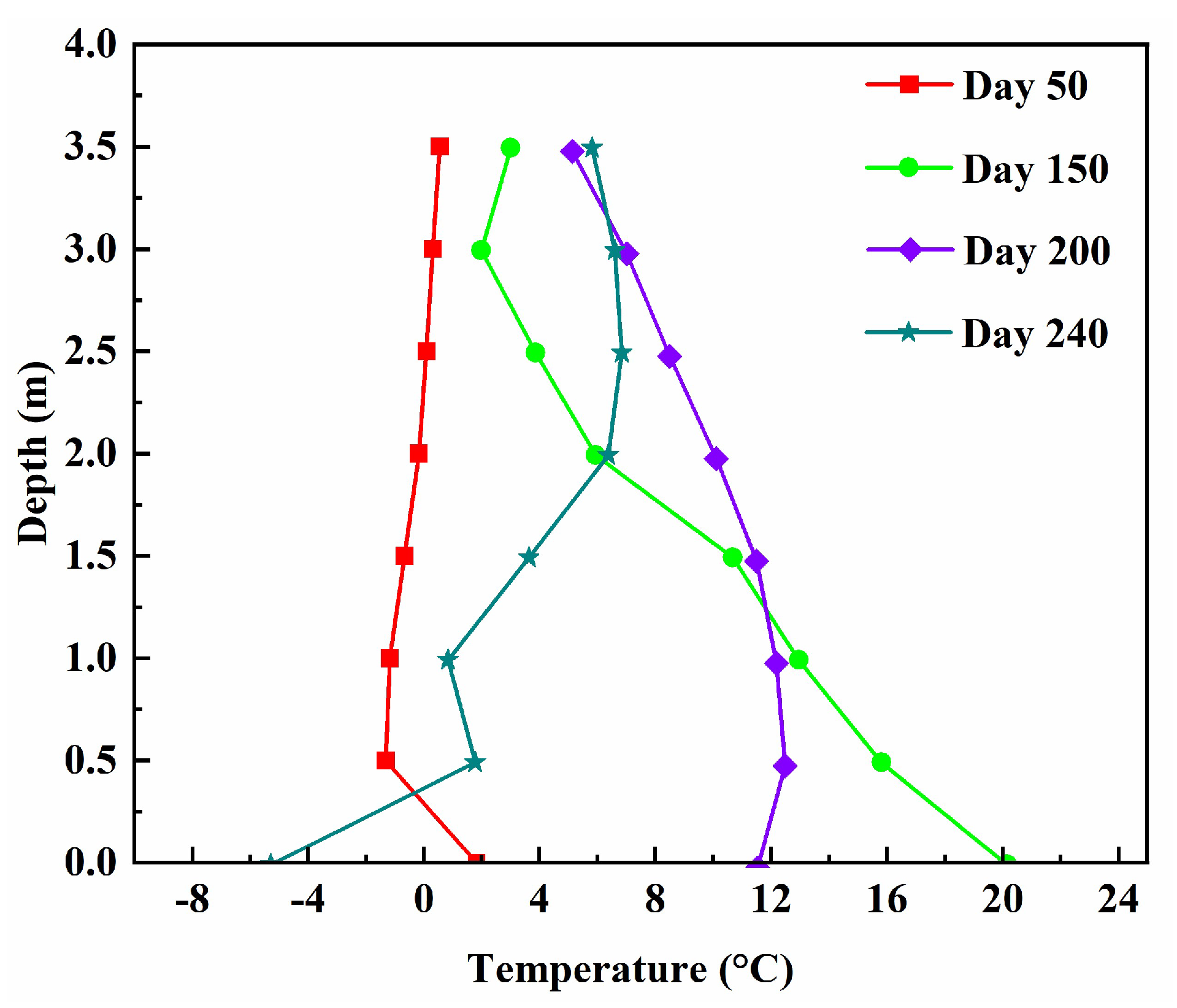
2.3. Model Validation

In order to verify the applicability of the above numerical model, a numerical simulation of the black soil freeze–thaw model test was conducted using the hydrothermal coupling method as described above as a means of verifying the applicability of the numerical model. This was done in conjunction with a black soil freeze–thaw model test conducted in the previous work of the authors [14], and then the results of the calculations were compared to the test results. In the developed computational model, the horizontal displacements and the bottom displacements on both lateral sides are restricted, whereas the upper surface of the model is designated as a free surface. The model dimensions are specified as having a length of 3.0 m and a height of 1.3 m. It was found that the initial temperature of the model test was 18 °C, the initial moisture content of the model test was 25.6%, and the temperature boundary conditions and moisture boundary conditions were consistent with the criteria used in the model test. It was simulated that the freezing stage process would take 306 h to complete, and the calculation time was set accordingly.

To investigate the temperature evolution in the black soil model test, Figure 1 presents a cloud diagram illustrating the distribution of temperature fields throughout the freezing process. As the ambient temperature decreases progressively, a temperature gradient emerges between the cold and warm ends of the soil. Concurrently, a portion of the liquid water undergoes a phase transition, resulting in the formation of ice crystals. The freezing front initiates at the cold end of the soil and progressively advances toward the warm end until it reaches its final position. A gradual increase in external ambient temperature will cause the soil to absorb a large amount of heat from the outside world, and as a consequence, the soil’s temperature will slowly rise. As the soil gradually thaws, the heat conduction reaches a state that eventually reaches a stable state, which forms a stable distribution of temperature fields.

The pattern of temperature change with time at different heights of the black soil model test can be found in the reference [14]. The freezing process induces the formation of a temperature gradient within the soil. This gradient facilitates the transfer of heat from regions of higher temperature to those of lower temperature, which in turn drives the movement of pore water toward the freezing front. Consequently, this movement results in the release of additional latent heat throughout the process. The temperature at different heights decreases with time and eventually reaches a steady state as time goes on. It is possible to divide the cooling process into three stages depending on how fast the freezing front is moving, namely rapid cooling, slow cooling, and the stabilization of the temperature. After 0–58 h, the soil temperature decreases rapidly, and the temperature difference between the top 10 cm of soil and the bottom 20 cm of soil is 31.957 °C, whereas the temperature difference between the top 20 cm of soil is 28.833 °C during this stage of rapid cooling. There was a temperature difference of 21.088 °C between the soil at 30 cm depth, 16.215 °C between soil at 40 cm depth, 12.963 °C between soil at 50 cm depth, 10.193 °C between soil at 60 cm depth, 9 °C between soil at 70 cm depth, and 8.49 °C between soil at 80 cm depth. After 58 h, the rate of temperature reduction gradually slowed down as well, and the temperatures in different parts of the soil body became closer to one another, indicating that the soil body had reached the slow cooling stage. A stable state is reached when the final temperature reaches a certain point, which belongs to the stabilization stage. The results of the numerical simulation of soil temperature in the freezing stage have been compared with the measured results of the test, and while there is a certain error in the numerical simulation value, the general trend of change in soil temperature in the freezing stage is the same. In the following paper, we demonstrate that the numerical simulation method we used in this study can be used to calculate the water–heat coupling of black soil roadbed slopes in the future.

Figure 2 depicts the moisture distribution within the black soil model throughout the frozen soil process, with the objective of enhancing the comprehension of moisture dynamics in this particular context. An analysis of the cloud diagram reveals that as the external ambient temperature progressively declines, a temperature gradient emerges between the colder and warmer ends of the soil. This temperature differential, coupled with the rapid freezing of water within the soil, impedes the movement of moisture. The freezing front keeps moving as time goes on and gradually advances to the warm part of the soil as the freezing time continues to go on. Under the driving force of the temperature gradient, water migrates from the lower part to the upper part of the soil, resulting in the formation of a stable moisture field distribution.

The distribution of ice content within the soil matrix is essential for examining the hydrothermal evolution of the soil. To gain a more comprehensive understanding of the changes in ice content during the freezing process in the black soil model test, a cloud diagram is presented in Figure 3. This diagram illustrates the distribution of ice content throughout the freezing process. As the internal temperature of the model reaches the freezing point, the liquid water transitions into ice. The cloud diagram indicates that, with the progression of freezing time, the ice content increases consistently from the top boundary to the bottom boundary of the model, reflecting the freezing process that occurs from the upper to the lower regions of the soil. It was evident from the beginning of the test that the temperatures near the top boundary were the first to decrease, leading to the formation of ice; at the end of the test, the growth rate of ice gradually decreased until it stopped completely. Ice impedance caused the soil to become blocked from allowing water to flow through the water migration channels, thereby affecting the process of water migration.

3. Analytical Model of Water–Heat Coupling of Black Soil Roadbed Slopes

3.1. Physical Parameter Values

As an example, we have established a hydrothermal finite element numerical model of a black soil roadbed in Heilongjiang Province based on the slope form of a black soil roadbed. In Figure 4, we can see that the slope was 20 m in height and the slope geometric model was constructed as a 2D geometric model. In order to improve the accuracy of the model calculation, the slope model meshing is based on a physical field control grid and the cell size is set to a very fine type in order to improve the accuracy of the model calculation. The values of the thermodynamic parameters of the soil samples were taken from the literature [1] and the values of the hydrodynamic parameters were calculated by referencing the literature [1], as shown in

Table 1. Computed parameters.

Parameter	Value	Unit	Parameter	Value	Unit
$C_s$	$2.20\times {10}^3$	$\mathrm{J}/\left(\mathrm{k}\mathrm{g}\cdot °\mathrm{C}\right)$	${\rho }_s$	$1.90\times {10}^3$	$\mathrm{k}\mathrm{g}/{\mathrm{m}}^3$
$C_w$	$4.180\times {10}^3$	$\mathrm{J}/\left(\mathrm{k}\mathrm{g}\cdot °\mathrm{C}\right)$	${\theta }_s$	$0.5$	$-$
$C_i$	$2.100\times {10}^3$	$\mathrm{J}/\left(\mathrm{k}\mathrm{g}\cdot °\mathrm{C}\right)$	${\theta }_r$	$0.02$	$-$
${\lambda }_{\mathrm{s}}$	$1.38$	$\mathrm{W}/\left(\mathrm{m}\cdot °\mathrm{C}\right)$	$T_f$	$-0.4$	$°\mathrm{C}$
${\lambda }_w$	$0.63$	$\mathrm{W}/\left(\mathrm{m}\cdot °\mathrm{C}\right)$	$B$	$0.56$	$-$
${\lambda }_i$	$2.31$	$\mathrm{W}/\left(\mathrm{m}\cdot °\mathrm{C}\right)$	$k_s$	$1\times {10}^{-8}$	$\mathrm{m}/\mathrm{s}$
$L$	$3.3456\times {10}^5$	$\mathrm{J}/\mathrm{k}\mathrm{g}$	$l$	$0.5$	$-$
${\rho }_i$	$0.918\times {10}^3$	$\mathrm{k}\mathrm{g}/{\mathrm{m}}^3$	$a$	$2.36$	$-$
${\rho }_w$	$1.000\times {10}^3$	$\mathrm{k}\mathrm{g}/{\mathrm{m}}^3$	$m$	$0.5$	$-$

, based on the values of the calculated parameters.

3.2. Boundary Conditions

There is a good match between the 2020–2021 temperature change in the study area and the local average temperature curve, and the entire trend of its graphical change approximates a sinusoidal curve, and we can express the fitted daily changes in average annual temperature as Equation (27).

$$T=0.75+23.8\sin ({\displaystyle \frac{2\pi }{365}}t-{\displaystyle \frac{\pi }{4}})$$

(27)

Temperature boundary conditions: Equation (27) is applied to the upper surface of the roadbed slope, with the lower surface temperature established at 3 °C. The lateral boundaries of the roadbed are assumed to be adiabatic, and the initial temperature is defined as 1 °C.

Moisture boundary condition: The analysis does not account for moisture loss due to external factors such as rainfall, snowmelt, and evaporation. Consequently, the moisture boundary condition for the roadbed slope is designated as zero flux during the simulation. The initial moisture content of the roadbed slope is set at 26.5%.

3.3. Analysis of Hydrothermal Evolution Pattern of Roadbed Slope

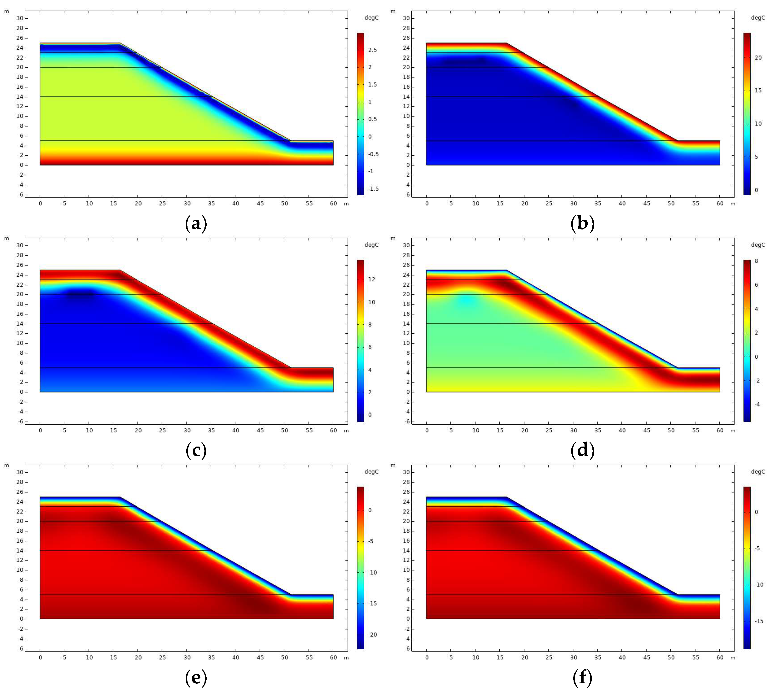
3.3.1. Temperature Field

In the course of this analysis, the loading time for the slope was initiated on 15 February 2020, representing the initial condition of the slope. The investigation focused on the variations in the temperature field of the slope over a one-year period to assess the alterations in slope temperature. As illustrated in Figure 5, the distribution of the temperature field within the roadbed slope is presented for 50 and 150 days post-initiation. It is evident that the temperature at the upper surface of the slope exhibits a gradual increase, correlating with the rise in external temperatures. Notably, significant changes occur within the shallow soil layer, extending to a depth of 2 m, while geothermal heat predominantly influences the deeper layers of the slope. Conversely, the data indicate that over a span of 200 days, the internal soil temperature continues to decline in response to decreasing external air temperatures. By the 240th day, measurements revealed that the upper surface temperature of the roadbed slope had fallen to sub-zero levels, signifying that the soil had entered a state of freezing at the time of observation. On the slope surface, the temperature distribution is very different, and there is a very small range in which the soil body has reached the freezing temperature, and there is a layer in the upper shallow layer of soil that is partially frozen. This is due to the downward transfer of cold energy, which will also result in the heat from the lower, warmer soil being transferred to the upper part, although the overall trend has not changed much over time. On the 330th day, the freezing line, defined as the contour at 0 °C, continues to descend within a slope that remains in the freezing phase, reflecting a gradual increase in freezing depth as the external ambient temperature experiences a slight decline. Conversely, on the 350th day, as external temperatures rise, the temperature at the upper surface of the slope also increases, resulting in a downward movement of the 0 °C isotherm. This indicates an expanding thawing depth corresponding to the gradual increase in external temperature. As the temperature of the slope’s soil body increases with depth, a general trend emerges wherein the temperature of the soil body decreases. This phenomenon can be attributed to the low external environmental temperatures during the freezing stage, which subsequently lower the temperature of the surface layer of the soil. Although there is a rise in external temperatures during the thawing stage, the temperature in the deeper layers of the soil remains elevated compared to that during the freezing stage. Consequently, a temperature gradient develops, transitioning from areas of higher temperature to those of lower temperature. This gradient facilitates the transfer of heat from the warmer regions to the cooler ones, thereby contributing to the observed thermal dynamics.

Commencing from the center of the roadbed slope, a systematic arrangement of sampling points was established along the vertical axis, with a precise interval of 0.5 m. This methodology aimed to thoroughly capture and analyze the temperature variations within the roadbed slope at various depths. Subsequently, a trend map illustrating the temperature changes with depth was generated based on the data obtained from these sampling points, as depicted in Figure 6. This visualization elucidates the complexity and regularity of temperature fluctuations with depth. A notable phenomenon of temperature variation was identified in the critical region of the side slope, extending from the surface layer to a depth of 2 m below ground level. This observation underscores the heightened sensitivity of the soil in this area to external environmental factors, including air temperature and humidity. As seasonal changes and subtle variations in external conditions occur, the temperature in this region exhibits a rapid response, reflecting corresponding fluctuations, which is crucial for understanding and predicting the stability of roadbed slopes. To further investigate the temperature change patterns of the roadbed slope, comparisons were made between the conditions of the slope after 50 days and 150 days. The comparative analysis revealed that as the external air temperature gradually increased, the temperature in the upper region of the slope exhibited a corresponding upward trend. This finding substantiates the significant impact of external air temperature on slope temperature. Over time, it was observed that the external air temperature began to decline as the observation progressed to the 200th day. In tandem, the temperature within the soil also continued to decrease, reinforcing the close correlation between slope temperature and external air temperature. At the critical juncture of the 240th day, the temperature at the slope’s surface fell below zero, indicating that the soil had officially transitioned into a frozen state. At this stage, the temperature distribution pattern of the slope’s surface layer underwent significant alterations, characterized by an increased temperature gradient and new patterns in the range and frequency of temperature fluctuations.

3.3.2. Moisture Field

An investigation was conducted to assess changes in the total volumetric water content of the slopes on the roadbed over the course of one year. It is essential to note that total volumetric water content encompasses both the volumetric water content of unfrozen water and that resulting from the transition of ice crystals to liquid water. Figure 7 illustrates the variations in the water field of the roadbed slope at intervals of 50, 150, and 200 days, reflecting the distribution of the water field. The data presented in the figure indicate that the water content within the shallow layer of the slope exhibits significant fluctuations, whereas the water content in the deeper layer remains consistently saturated throughout the observed period. As of the 240th day, a small amount of water already has been accumulated on the slope surface. This is due to the fact that at the beginning stages of soil freezing, the surface layer of the slope begins to freeze, and its water content begins to decrease, which is evident in the early stages of soil freezing, as well as the fact that the deeper layers of the soil are not yet frozen and have a greater amount of water than those of the shallow layers. A poly-ice region was observed at a depth of 2 m beneath the roadbed on the 330th day, attributed to the migration of moisture from the unfrozen section of the roadbed to the frozen section. Following the conclusion of the freezing period, the water content within the shallow soil layer exhibited a rapid decline. Nevertheless, it is noteworthy that, despite this decline, the overall water content of the shallow soil layer remained relatively stable at the end of the freezing process. The melted soil of the roadbed began to melt on the 350th day, and the melted water migrated downward by gravity, but the lower layer of soil had not yet melted, which prevented the water from migrating downward, so the water content of the soil surface increased as a result.

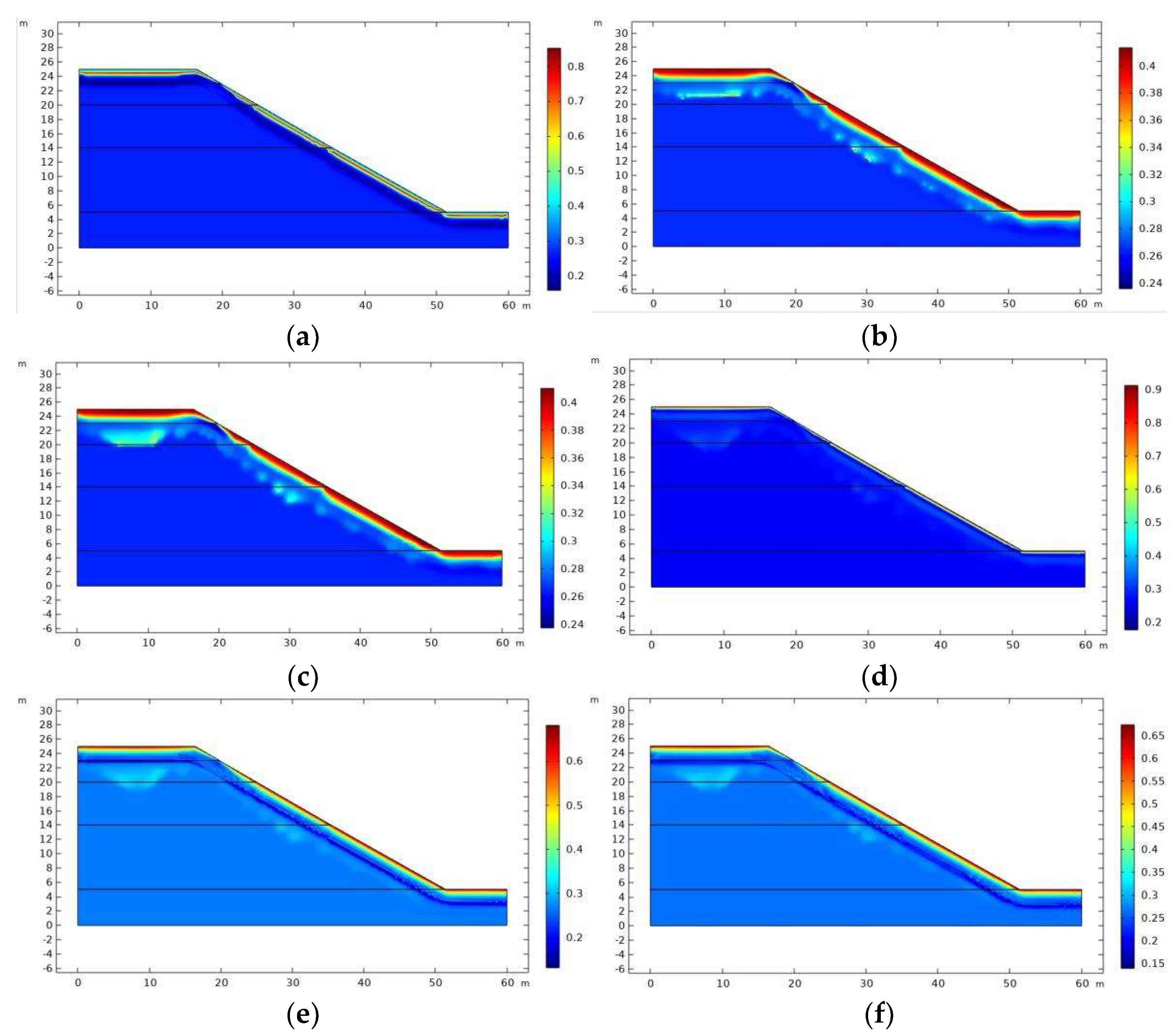
3.3.3. Distribution of Ice Content

As a result of the freezing and thawing of soils over time, both water and ice are converted into each other, and the latent heat associated with phase transition is released and absorbed in a unique process related to freezing and thawing. Due to soil water migration and phase changes, the amount of soil ice can become too high, resulting in the freezing and thawing of the soil. The ice content is a critical parameter in the study of frozen soil, as it plays a significant role in understanding the mechanisms of freezing and thawing damage in roadbed slopes. This paper presents an analysis of the distribution of ice content within these slopes. Figure 8 illustrates a cloud diagram depicting the volumetric ice content of the roadbed slope. On the 240th day of observation, the soil temperature drops below zero, leading to a corresponding decrease in the upper surface temperature of the slope. This temperature decline initiates the freezing process, resulting in the formation of a partially frozen layer in the uppermost shallow region and an increase in the volumetric ice content of the slope. By the 330th day of the experiment, the soil remains in a freezing state, as the cold energy continues to facilitate the formation of ice lenses over time. However, as the external air temperature gradually rises by the 350th day, the upper surface temperature of the slope begins to recover, leading to the gradual melting of the ice lenses.

4. Conclusions

This study aims to investigate the water–heat coupling dynamics associated with the freezing and thawing processes of black soil in regions characterized by seasonal frost, with a particular focus on elucidating the mechanisms underlying the damage to black soil roadbed slopes during these cycles. The analysis employs principles of mass conservation, energy conservation, Darcy’s law pertaining to unsaturated soil water flow, and heat conduction theory. Through mathematical transformations, a theoretical model representing the water–heat coupling of black soil in seasonal frozen environments is developed, incorporating definitions of relative saturation and the solid–liquid ratio. A black soil freeze–thaw model test was conducted to verify the model’s validity, with a further analysis of temperature field, moisture field, and ice content distribution generated by the phase change process during the freeze–thaw process. The main conclusions are as follows:

(1)

According to the numerical model, the temperature field obtained during freezing and thawing in seasonal frozen soil regions is accurate and able to simulate the temperature field, moisture field, and ice content distribution law of black soil.

(2)

In the context of black soil roadbed slopes that have not yet reached the freezing threshold, an increase in external air temperature results in a corresponding rise in surface temperature at the upper section of the slope. The shallow 2 m layer of the slope exhibits significant fluctuations, while geothermal heat predominantly influences the deeper layers. Once the roadbed slope attains the freezing point, the 0 °C isotherm descends as the external ambient temperature gradually declines. Conversely, as external air temperatures rise, the surface temperature of the upper slope increases progressively, leading to an expansion in the thawing depth.

(3)

Black soil roadbed slopes with shallow water layers that have not reached the freezing point demonstrate considerable variations in water content in response to changes in external air temperature. During the freezing phase, the surface layer of the slope begins to freeze, resulting in a decrease in water content at the surface and the formation of a poly-ice zone approximately 2 m beneath the surface. In the subsequent melting phase, the roadbed slope undergoes thawing, allowing water to flow downward under the influence of gravity. However, since the lower soil layer remains frozen, the water is unable to migrate downward, leading to an accumulation of water content at the soil surface.

(4)

The distribution of ice content within black soil roadbeds during phase transitions is characterized by the formation of a partially frozen soil layer in the upper shallow section of the slope, which results in a gradual increase in volumetric ice content at the slope’s surface. As external air temperatures rise, the temperature of the upper surface of the slope gradually recovers, reaching the freezing point and initiating the melting process, which ultimately leads to the disappearance of ice lenses.

References

1. Xu, X.; Wang, J.C.; Zhang, L.X. Frozen Soil Physics; Science Press: Beijing, China, 2001. [Google Scholar]
2. Ling, X.; Zhang, F.; Zhu, Z.; Ding, L.; Hu, Q. Field experiment of subgrade vibration induced by passing train in a seasonally frozen region of Daqing. Earthq. Eng. Eng. Vib. 2009, 8, 149–157. [Google Scholar] [CrossRef]
3. Ling, X.Z.; Chen, S.J.; Zhu, Z.Y.; Zhang, F.; Wang, L.N.; Zou, Z.Y. Field monitoring on the train-induced vibration response of track structure in the Beiluhe permafrost region along Qinghai–Tibet railway in China. Cold Reg. Sci. Technol. 2010, 60, 75–83. [Google Scholar] [CrossRef]
4. Wang, M.; Meng, S.; Yuan, X.; Sun, Y.; Zhou, J. Experimental validation of vibration-excited subsidence model of seasonally frozen soil under cyclic loads. Cold Reg. Sci. Technol. 2018, 146, 175–181. [Google Scholar] [CrossRef]
5. Wang, M.; Meng, S.; Sun, Y.; Fu, H. Shear strength of frozen clay under freezing-thawing cycles using triaxial tests. Earthq. Eng. Eng. Vib. 2018, 17, 761–769. [Google Scholar] [CrossRef]
6. Liu, T.; Wang, M. Experimental research on the development of residual strain in seasonal frozen soil under freezing-thawing and impact type traffic loads. Earthq. Eng. Eng. Vib. 2021, 20, 335–345. [Google Scholar]
7. Leng, J.; Fu, X.; Yang, J. Experimental research of the subgrade padding frost heaving of high-speed railway. J. Glaciol. Geocryol. 2015, 37, 440–445. [Google Scholar]
8. Wang, Q.; Liu, J.; Tian, Y.; Fang, J.; Zhu, X. A study of orthogonal design tests on frost-heaving characteristics of graded crushed rock. Rock Soil Mech. 2015, 36, 2825–2830. [Google Scholar]
9. Wang, Y.; Wang, D.; Guo, Y.; Lei, L.; Gu, T. Experimental study of the development characteristic of frost heaving ratio of of the saturated Tibetan silt under one-dimensional freezing. J. Glaciol. Geocryol. 2016, 38, 409–415. [Google Scholar]
10. She, W.; Wei, L.; Zhao, G.; Yang, G.; Jiang, J.; Hong, J. New insights into the frost heave behavior of coarse grained soils for high-speed railway roadbed: Clustering effect of fines. Cold Reg. Sci. Technol. 2019, 167, 102863. [Google Scholar] [CrossRef]
11. Jin, H.W.; Lee, J.; Ryun, H.; Shin, Y.; Jang, Y.E. Experimental Assessment of the Effect of Frozen Fringe Thinkness on Frost Heave. Geomech. Eng. 2019, 19, 193–199. [Google Scholar]
12. Luo, Q.; Wu, P.; Wang, T. Evaluating frost heave susceptibility of well-graded gravel for HSR subgrade based on orthogonal array testing. Transp. Geotech. 2019, 21, 100283. [Google Scholar] [CrossRef]
13. Yu, L.; Xu, X.; Ma, C. Combination effect of seasonal freezing and artificial freezing on frost heave of silty clay. J. Cent. South Univ. Technol. 2010, 17, 163–168. [Google Scholar] [CrossRef]
14. Hai, M.; Su, A.; Wang, M.; Gao, S.; Lu, C.; Guo, Y.; Xiao, C. Large-Scale Freezing and Thawing Model Experiment and Analysis of Water–Heat Coupling Processes in Agricultural Soils in Cold Regions. Water 2023, 16, 19. [Google Scholar] [CrossRef]
15. Wang, M.; Hai, M.; Su, A.; Meng, S.; Mu, H.; Guo, Y. Experimental Study on the Effect of Fines Content on the Frost Swelling Characteristics of Coarse-Grained Soil in Canal Base Under Open System. J. Offshore Mech. Arct. Eng. 2024, 146, 022101. [Google Scholar] [CrossRef]
16. Wang, M.; Hai, M.; Su, A.; Xu, J.; Guo, Y.; Yan, H. Study of hydrothermal characteristics of large-scale water conveyance trunk canals in seasonally frozen ground regions under the influence of different initial water contents. River 2024, 3, 166–180. [Google Scholar] [CrossRef]
17. Li, Z.; Chen, J.; Sugimoto, M.; Ge, H. Numerical simulation model of artificial ground freezing for tunneling under seepage flow conditions. Tunn. Undergr. Space Technol. 2019, 92, 103035. [Google Scholar] [CrossRef]
18. Li, X.K.; Li, X.; Liu, S.; Qi, J.L. Thermal-seepage coupled numerical simulation methodology for the artificial ground freezing process. Comput. Geotech. 2023, 156, 105246. [Google Scholar] [CrossRef]
19. Lai, Y.; Pei, W.; Zhang, M.; Zhou, J. Study on theory model of hydro-thermal–mechanical interaction process in saturated freezing silty soil. Int. J. Heat Mass Transf. 2014, 78, 805–819. [Google Scholar] [CrossRef]
20. Harlan, R.L. Analysis of coupled heat-fluid transport in partially frozen soil. Water Resour. Res. 1973, 9, 1314–1323. [Google Scholar] [CrossRef]
21. Bai, R.; Lai, Y.; Zhang, M.; Yu, F. Theory and application of a novel soil freezing characteristic curve. Appl. Therm. Eng. 2018, 129, 1106–1114. [Google Scholar] [CrossRef]
22. Tan, X.; Chen, W.; Tian, H.; Cao, J. Water flow and heat transport including ice/water phase change in porous media: Numerical simulation and application. Cold Reg. Sci. Technol. 2011, 68, 74–84. [Google Scholar] [CrossRef]
23. Tai, B.; Liu, J.; Wang, T.; Shen, Y.; Li, X. Numerical modelling of anti-frost heave measures of high-speed railway subgrade in cold regions. Cold Reg. Sci. Technol. 2017, 141, 28–35. [Google Scholar] [CrossRef]
24. Zhou, J.; Li, D. Numerical analysis of coupled water, heat and stress in saturated freezing soil. Cold Reg. Sci. Technol. 2012, 72, 43–49. [Google Scholar] [CrossRef]
25. Wang, T.; Liu, J.; Tai, B.; Zang, C.; Zhang, Z. Frost jacking characteristics of screw piles in seasonally frozen regions based on thermo-mechanical simulations. Comput. Geotech. 2017, 91, 27–38. [Google Scholar] [CrossRef]
26. Zhou, Y.; Zhou, G. Numerical simulation of coupled heat-fluid transport in freezing soils using finite volume method. Heat Mass Transf. 2010, 46, 989–998. [Google Scholar] [CrossRef]
27. Li, S.; Lai, Y.; Pei, W.; Zhang, S.; Zhong, H. Moisture–temperature changes and freeze–thaw hazards on a canal in seasonally frozen regions. Nat. Hazards 2014, 72, 287–308. [Google Scholar] [CrossRef]
28. Ren, Z.; Liu, J.; Jiang, H.; Wang, E. Experimental study and simulation for unfrozen water and compressive strength of frozen soil based on artificial freezing technology. Cold Reg. Sci. Technol. 2023, 205, 103711. [Google Scholar] [CrossRef]
29. Sun, Y.; Zhou, S.; Meng, S.; Wang, M.; Bai, H. Accumulative plastic strain of freezing-thawing subgrade clay under cyclic loading and its particle swarm optimization-back-propagation-based prediction model. Cold Reg. Sci. Technol. 2023, 214, 103946. [Google Scholar] [CrossRef]
30. Sun, Y.; Zhou, S.; Meng, S.; Wang, M.; Mu, H. Principal component analysis–artificial neural network-based model for predicting the static strength of seasonally frozen soils. Sci. Rep. 2023, 13, 16085. [Google Scholar] [CrossRef]
31. Wang, Q.; Bai, R.; Zhou, Z.; Zhu, W. Evaluating thermal conductivity of soil-rock mixtures in Qinghai-Tibet plateau based on theory models and machine learning methods. Int. J. Therm. Sci. 2024, 204, 109210. [Google Scholar] [CrossRef]
32. Cheng, K.; Ping, X.; Han, B.; Wu, H.; Liu, H. Study on particle loss-induced deformation of gap-graded soils: Role of particle stress. Acta Geotech. 2024, 1–28. [Google Scholar] [CrossRef]
33. Chang, D.; Yan, Y.; Liu, J.; Xu, A.; Feng, L.; Zhang, M. Micro-macroscopic mechanical behavior of frozen sand based on a large-scale direct shear test. Comput. Geotech. 2023, 159, 105484. [Google Scholar] [CrossRef]
34. Yan, Y.; Chang, D.; Liu, J.; Xu, A.; Zhang, M.; Xie, Y. Design and validation of a new temperature-controlled large-scale direct shear apparatus. Cold Reg. Sci. Technol. 2023, 216, 103992. [Google Scholar] [CrossRef]
35. Yan, Y.; Chang, D.; Liu, J.; Xu, A. Multiscale mechanical analysis of Frozen Clay: Triaxial testing and discrete element modeling. Cold Reg. Sci. Technol. 2024, 224, 104250. [Google Scholar] [CrossRef]
36. Wu, H.; Shi, A.; Ni, W.; Zhao, L.; Cheng, Z.; Zhong, Q. Numerical simulation on potential landslide–induced wave hazards by a novel hybrid method. Eng. Geol. 2024, 331, 107429. [Google Scholar] [CrossRef]
37. Taylor, G.S.; Luthin, J.N. A model for coupled heat and moisture transfer during soil freezing. Can. Geotech. J. 1978, 15, 548–555. [Google Scholar] [CrossRef]
38. Van Genuchten, M.T. A closed-form equation for predicting the hydraulic conductivity of unsaturated soils. Soil Sci. Soc. Am. J. 1980, 44, 892–898. [Google Scholar] [CrossRef]
39. Gardner, W.R. Some steady-state solutions of the unsaturated moisture flow equation with application to evaporation from a water table. Soil Sci. 1958, 85, 228–232. [Google Scholar] [CrossRef]
40. Comsol, A.B. COMSOL multiphysics user’s guide. Version Sept. 2005, 10, 333. [Google Scholar]
Figure 1. Cloud view of the temperature field of the black soil model test: (a) 40 h; (b) 80 h; and (c) 218 h.
Sustainability 16 08427 g001
Figure 2. Cloud map of moisture field in black soil modeling test: (a) 40 h; (b) 80 h; and (c) 218 h.
Sustainability 16 08427 g002
Figure 3. Cloud map of ice content in black soil modeling tests: (a) 40 h; (b) 80 h; and (c) 218 h.
Sustainability 16 08427 g003
Figure 4. Black soil roadbed slope modeling diagram.
Sustainability 16 08427 g004
Figure 5. Temperature field distribution of roadbed slopes: (a) day 50; (b) day 150; (c) day 200; (d) day 240; (e) day 330; and (f) day 350.
Sustainability 16 08427 g005
Figure 6. Distribution of moisture field of roadbed slope.
Sustainability 16 08427 g006
Figure 7. Distribution of moisture field of roadbed slope: (a) day 50; (b) day 150; (c) day 200; (d) day 240; (e) day 330; and (f) day 350.
Sustainability 16 08427 g007
Figure 8. Ice content distribution of roadbed slopes: (a) day 240; (b) day 330; and (c) day 350.
Sustainability 16 08427 g008