
Land Use Intensity Alters Ecosystem Service Supply and Demand as Well as Their Interaction: A Spatial Zoning Perspective


Abstract
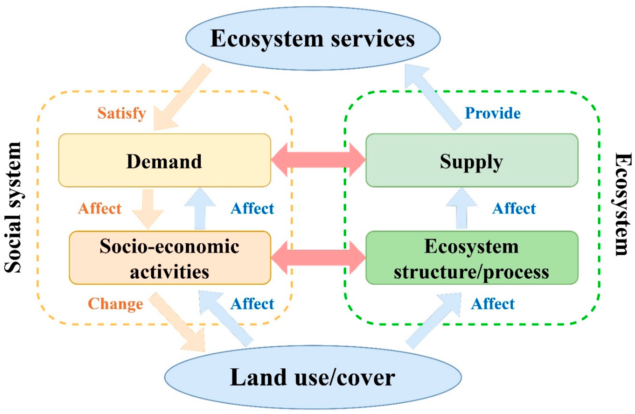
1. Introduction
2. Materials and Methods
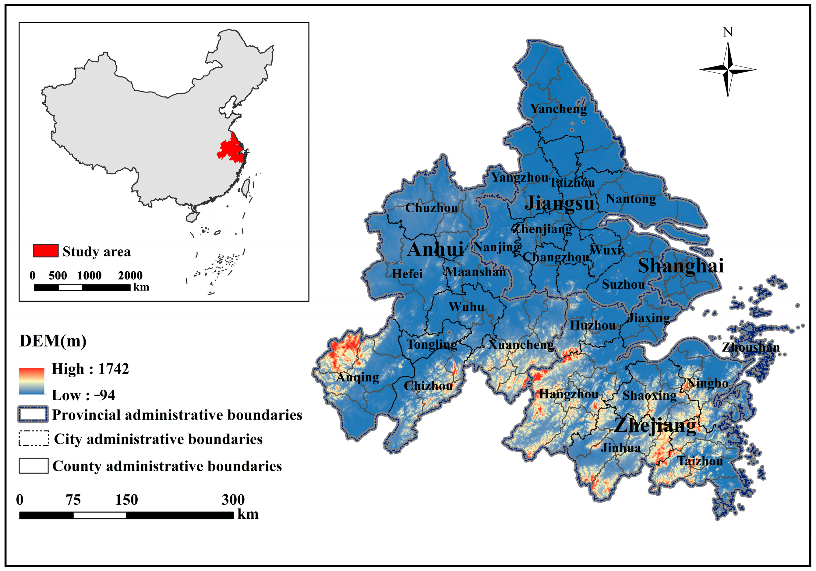
2.1. Study Area
2.2. Data Sources
2.3. Methods
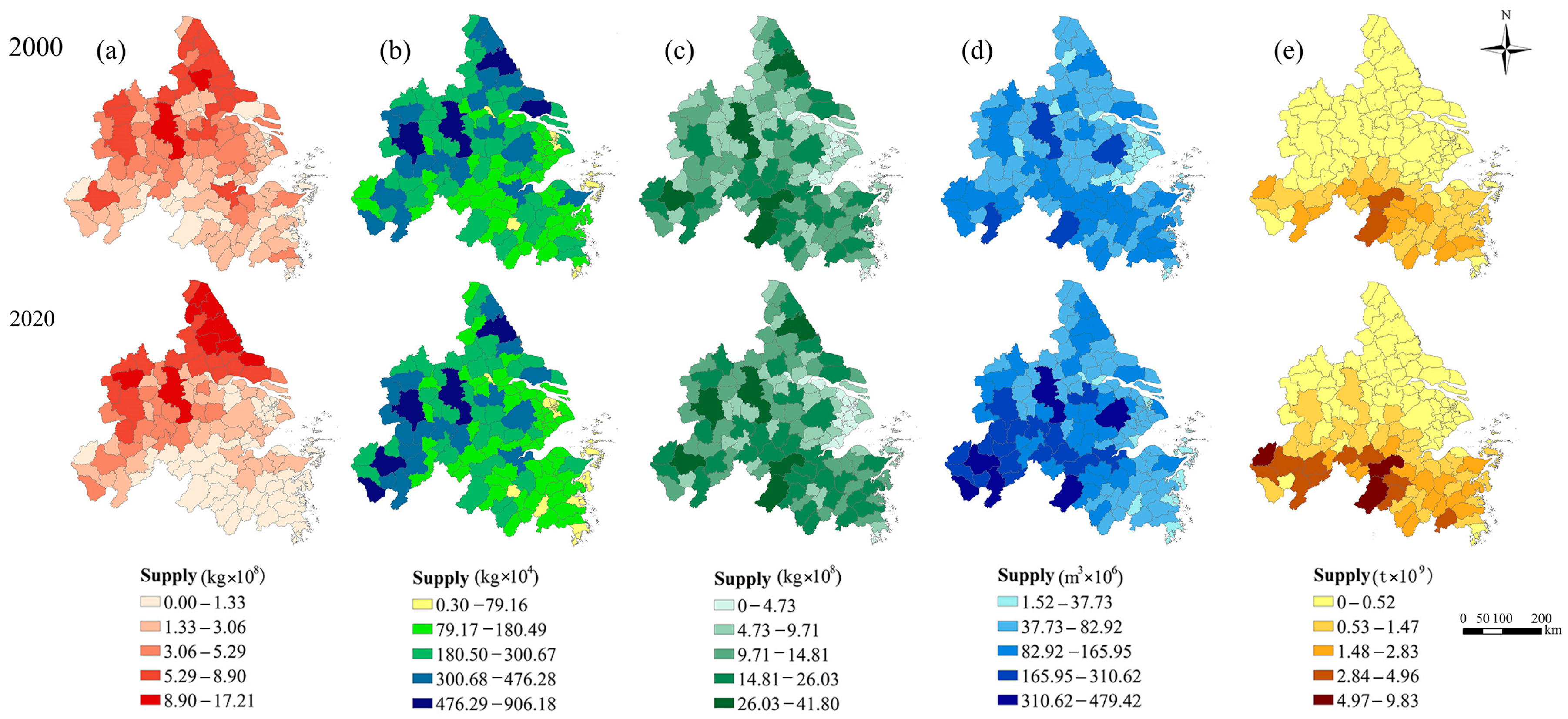
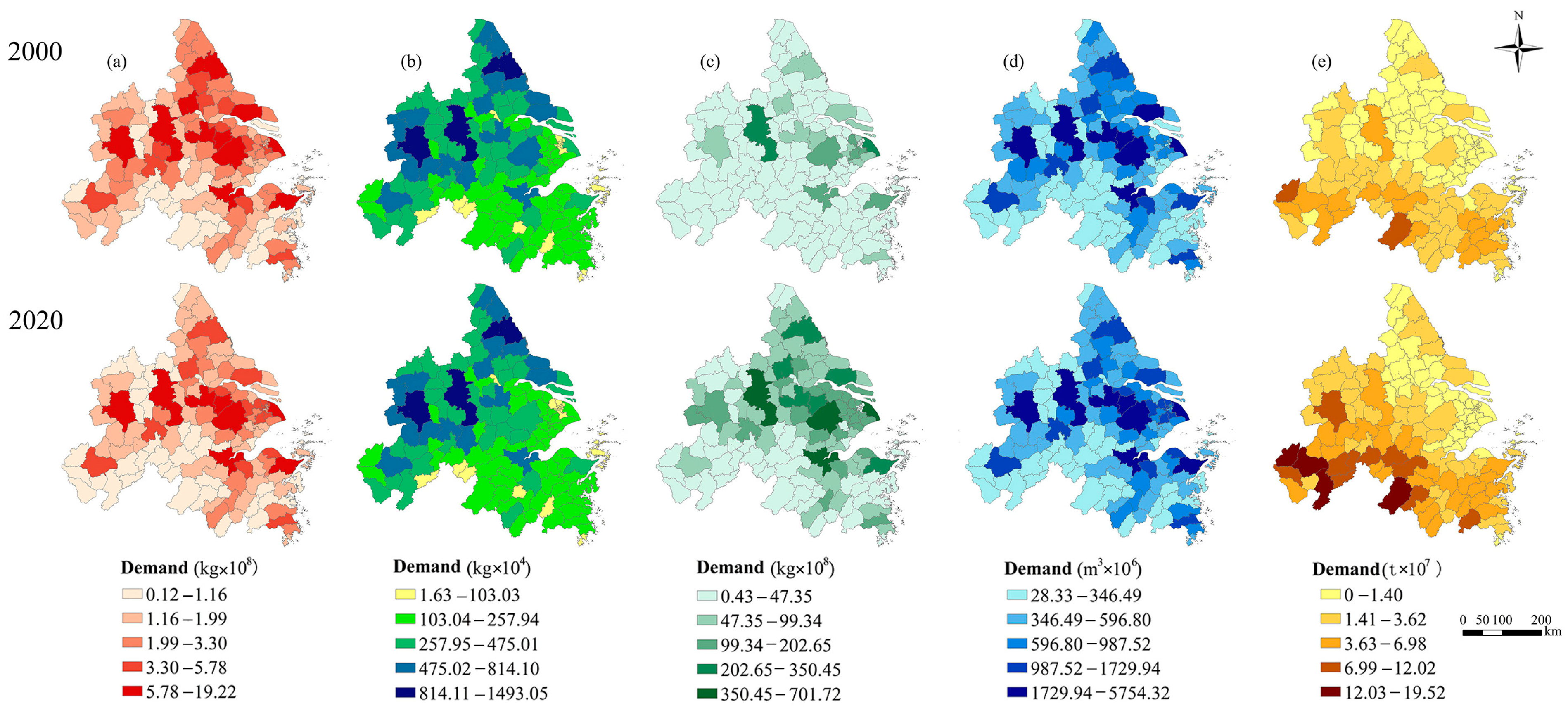
2.3.1. Measurement of ESS and ESD
- (a)
- Food supply
- (b)
- Water purification
- (c)
- Carbon sequestration
- (d)
- Water conservation
- (e)
- Soil retention
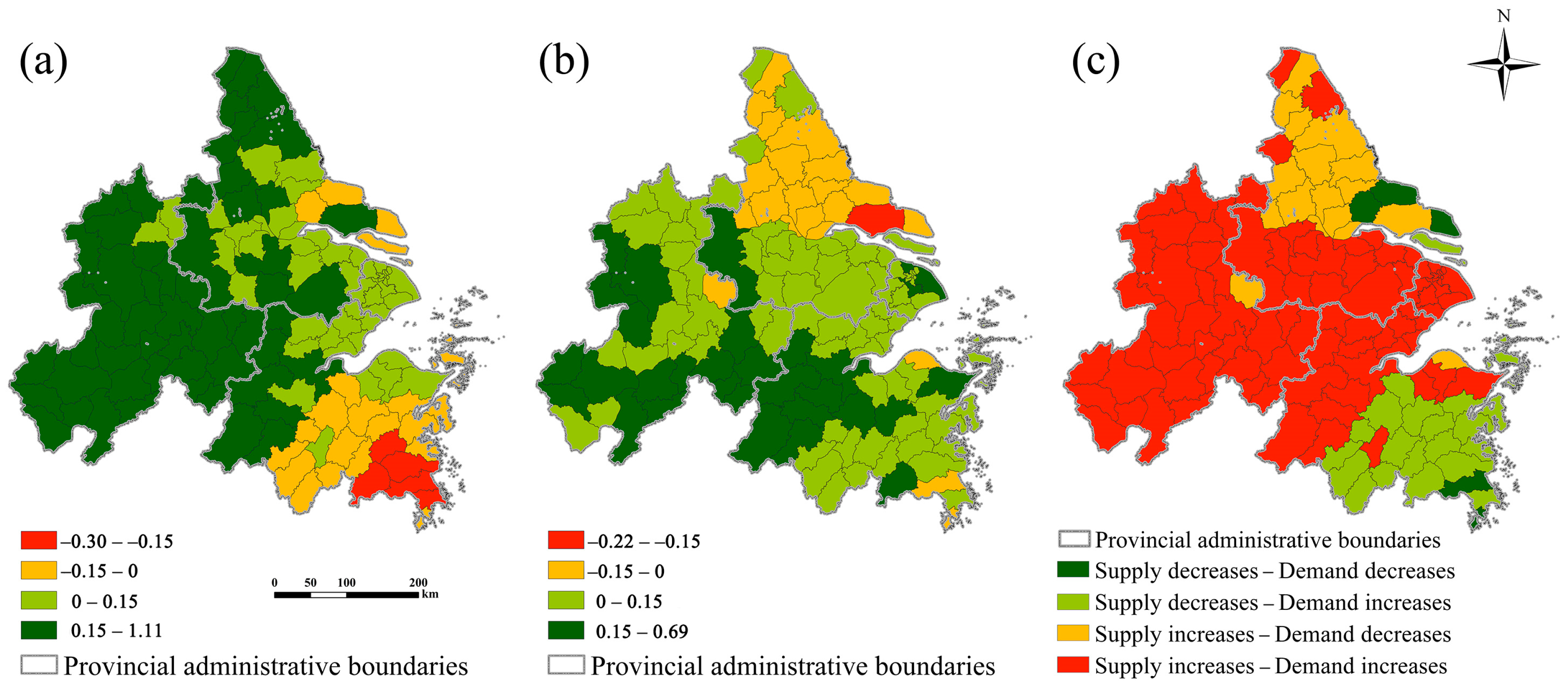
2.3.2. Spatial Zoning Based on Changes in ESs
2.3.3. Interaction between ESS and ESD
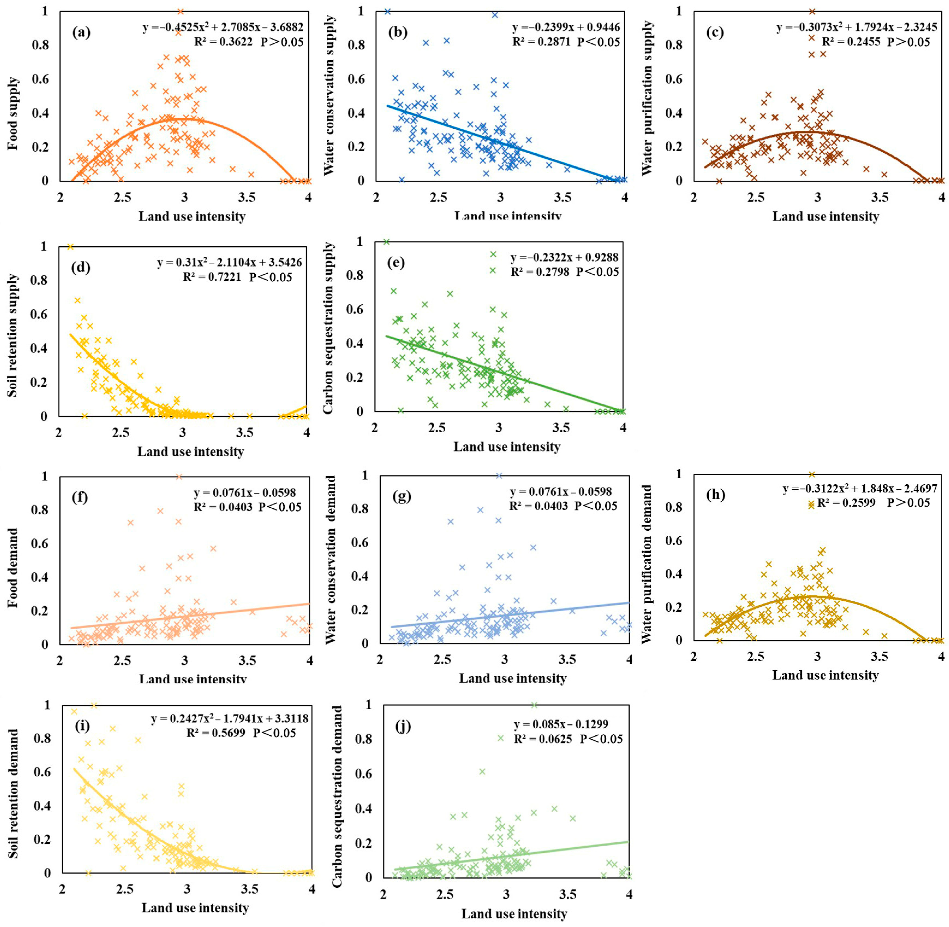
2.3.4. The Influence of Land Use Intensity on ESs
3. Results
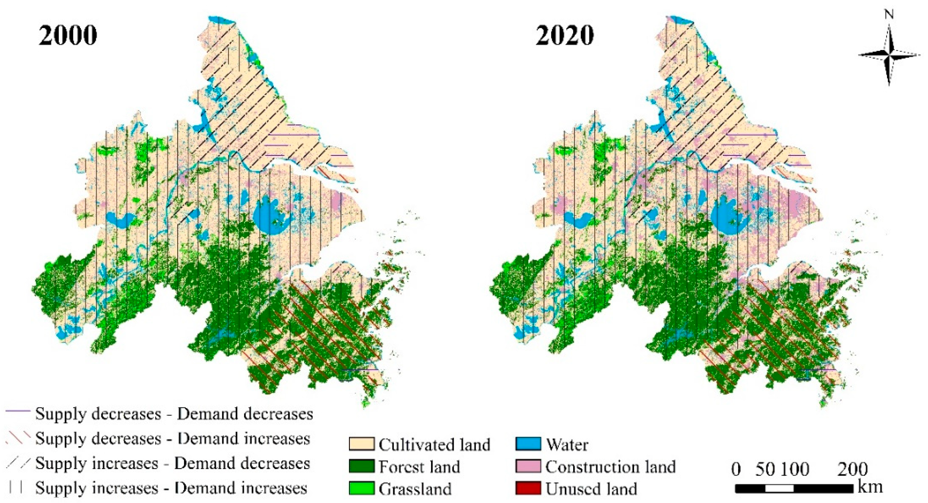
3.1. Land Use Change from 2000 to 2020
3.2. Spatial Zoning of Changes in ESS and ESD
3.3. Interaction between ESS and ESD
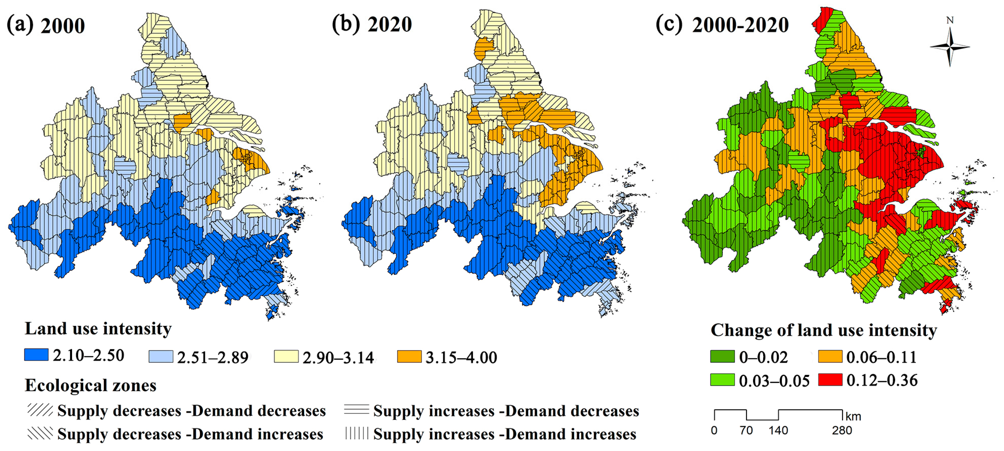
3.4. Influence of LUI on ESS and ESD
4. Discussion
4.1. Potential Influence of Land Use Change on Supply–Demand Interaction
4.2. Policy Implications
4.3. Limitations and Prospects
5. Conclusions
Author Contributions
Funding
Institutional Review Board Statement
Informed Consent Statement
Data Availability Statement
Conflicts of Interest
References
- Costanza, R.; D’Arge, R.; de Groot, R.; Farber, S.; Grasso, M.; Hannon, B.; Limburg, K.; Naeem, S.; O’Neill, R.V.; Paruelo, J.; et al. The value of the world’s ecosystem services and natural capital. Nature 1997, 387, 253–260. [Google Scholar] [CrossRef]
- Costanza, R.; de Groot, R.; Braat, L.; Kubiszewski, I.; Fioramonti, L.; Sutton, P.; Farber, S.; Grasso, M. Twenty years of ecosystem services: How far have we come and how far do we still need to go? Ecosyst. Serv. 2017, 28, 1–16. [Google Scholar] [CrossRef]
- Daily, G.C. Nature’s Services: Societal Dependence on Natural Eco-Systems; Island Press: Washington, DC, USA, 1997. [Google Scholar]
- MA (Millennium Ecosystem Assessment). Ecosystems and Human Well-Being; Island Press: Washington, DC, USA, 2005. [Google Scholar]
- Castro, A.J.; Verburg, P.H.; Martín-López, B.; Garcia-Llorente, M.; Cabello, J.; Vaughn, C.C.; López, E. Ecosystem service trade-offs from supply to social demand: A landscape-scale spatial analysis. Landsc. Urban Plan. 2014, 132, 102–110. [Google Scholar] [CrossRef]
- Ouyang, Z.Y.; Zheng, H.; Xiao, Y.; Polasky, S.; Liu, J.G.; Xu, W.H.; Wang, Q.; Zhang, L.; Xiao, Y.; Rao, E.M.; et al. Improvements in ecosystem services from investments in natural capital. Science 2016, 352, 1455–1459. [Google Scholar] [CrossRef]
- Sun, R.; Jin, X.B.; Han, B.; Liang, X.Y.; Zhang, X.L.; Zhou, Y.K. Does scale matter? Analysis and measurement of ecosystem service supply and demand status based on ecological unit. Environ. Impact Assess. Rev. 2022, 95, 106785. [Google Scholar] [CrossRef]
- Burkhard, B.; Kroll, F.; Nedkov, S.; Müller, F. Mapping ecosystem service supply, demand and budgets. Ecol. Indic. 2012, 21, 17–29. [Google Scholar] [CrossRef]
- Wolff, S.; Schulp, C.J.E.; Verburg, P.H. Mapping ecosystem services demand: A review of current research and future perspectives. Ecol. Indic. 2015, 55, 159–171. [Google Scholar] [CrossRef]
- Zhang, J.; Li, S.; Lin, N.; Lin, Y.; Yuan, S.; Zhang, L.; Zhu, J.; Wang, K.; Gan, M.; Zhu, C. Spatial identification and trade-off analysis of land use functions improve spatial zoning management in rapid urbanized areas, China. Land Use Policy 2022, 116, 106058. [Google Scholar] [CrossRef]
- Ayanu, Y.Z.; Conrad, C.; Nauss, T.; Wegmann, M.; Koellner, T. Quantifying and mapping ecosystem services supplies and demands: A review of remote sensing applications. Environ. Sci. Technol. 2012, 46, 8529–8541. [Google Scholar] [CrossRef]
- Lyu, R.F.; Clarke, K.C.; Zhang, J.M.; Feng, J.L.; Jia, X.H.; Li, J.J. Spatial correlations among ecosystem services and their socio-ecological driving factors: A case study in the city belt along the Yellow River in Ningxia, China. Appl. Geogr. 2019, 108, 64–73. [Google Scholar] [CrossRef]
- Meng, J.J.; Cheng, H.R.; Li, F.; Han, Z.Y.; Wei, C.J.; Wu, Y.D.; You, N.W.; Zhu, L.K. Spatial-temporal trade-offs of land multi-functionality and function zoning at finer township scale in the middle reaches of the Heihe River. Land Use Policy 2022, 115, 106019. [Google Scholar] [CrossRef]
- Lapointe, M.; Gurney, G.G.; Cumming, G.S. Urbanization affects how people perceive and benefit from ecosystem service bundles in coastal communities of the Global South. Ecosyst. People 2021, 17, 57–68. [Google Scholar] [CrossRef]
- Schirpke, U.; Candiago, S.; Vigl, L.E.; Jäger, H.; Labadini, A.; Marsoner, T.; Meisch, C.; Tasser, E.; Tappeiner, U. Integrating supply, flow and demand to enhance the understanding of interactions among multiple ecosystem services. Sci. Total Environ. 2019, 651, 928–941. [Google Scholar] [CrossRef] [PubMed]
- Wang, L.; Gong, J.; Ma, S.; Wu, S.; Zhang, X.; Jiang, J. Ecosystem service supply-demand and socioecological drivers at different spatial scales in Zhejiang Province, China. Ecol. Indic. 2022, 140, 109058. [Google Scholar] [CrossRef]
- Ala-Hulkko, T.; Kotavaara, O.; Alahuhta, J.; Hjort, J. Mapping supply and demand of a provisioning ecosystem service across Europe. Ecol. Indic. 2019, 103, 520–529. [Google Scholar] [CrossRef]
- Nedkov, S.; Burkhard, B. Flood regulating ecosystem services—Mapping supply and demand, in the Etropole municipality, Bulgaria. Ecol. Indic. 2012, 21, 67–79. [Google Scholar] [CrossRef]
- Xu, Z.H.; Peng, J.; Dong, J.Q.; Liu, Y.X.; Liu, Q.Y.; Lyu, D.; Qiao, R.L.; Zhang, Z.M. Spatial correlation between the changes of ecosystem service supply and demand: An ecological zoning approach. Landsc. Urban Plan. 2022, 217, 104258. [Google Scholar] [CrossRef]
- Baró, F.; Gómez-Baggethun, E.; Haase, D. Ecosystem service bundles along the urban-rural gradient: Insights for landscape planning and management. Ecosyst. Serv. 2017, 24, 147–159. [Google Scholar] [CrossRef]
- Xia, H.; Yuan, S.F.; Prishchepov, A.V. Spatial-temporal heterogeneity of ecosystem service interactions and their social-ecological drivers: Implications for spatial planning and management. Resour. Conserv. Recycl. 2023, 189, 106767. [Google Scholar] [CrossRef]
- García-Llorente, M.; Iniesta-Arandia, I.; Willaarts, B.A.; Harrison, P.A.; Berry, P.; Del Mar Bayo, M.; Castro, A.J.; Montes, C.; Martín-López, B. Biophysical and sociocultural factors underlying spatial trade-offs of ecosystem services in semiarid watersheds. Ecol. Soc. 2015, 20, 39. [Google Scholar] [CrossRef]
- Wang, Z.B.; Liang, L.W.; Sun, Z.; Wang, X.M. Spatiotemporal differentiation and the factors influencing urbanization and ecological environment synergistic effects within the Beijing-Tianjin-Hebei urban agglomeration. J. Environ. Manag. 2019, 243, 227–239. [Google Scholar] [CrossRef] [PubMed]
- Zhao, Y.N.; Wang, M.; Lan, T.H.; Xu, Z.H.; Wu, J.S.; Liu, Q.Y.; Peng, J. Distinguishing the effects of land use policies on ecosystem services and their trade-offs based on multi-scenario simulations. Appl. Geogr. 2023, 151, 102864. [Google Scholar] [CrossRef]
- Roces-Díaz, J.V.; Vayreda, J.; Banqué-Casanovas, M.; Díaz-Varela, E.; Bonet, J.A.; Brotons, L.; De-Miguel, S.; Herrando, S.; Martínez-Vilalta, J. The spatial level of analysis affects the patterns of forest ecosystem services supply and their relationships. Sci. Total Environ. 2018, 626, 1270–1283. [Google Scholar] [CrossRef]
- Yang, Y.J.; Wang, K.; Liu, D.; Zhao, X.Q.; Fan, J.W. Effects of land-use conversions on the ecosystem services in the agro-pastoral ecotone of northern China. J. Clean. Prod. 2019, 249, 119360. [Google Scholar] [CrossRef]
- Jiang, B.; Bai, Y.; Chen, J.Y.; Alatalo, J.; Xu, X.B.; Liu, G.; Wang, Q. Land management to reconcile ecosystem services supply and demand mismatches-A case study in Shanghai municipality, China. Land Degrad. Dev. 2020, 31, 2684–2699. [Google Scholar] [CrossRef]
- Chillo, V.; Vázquez, D.P.; Amoroso, M.M.; Bennett, E.M. Land use intensity indirectly affects ecosystem services mainly through plant functional identity in a temperate forest. Funct. Ecol. 2018, 32, 1390–1399. [Google Scholar] [CrossRef]
- Song, W.; Deng, X.Z. Land-use/land-cover change and ecosystem service provision in China. Sci. Total Environ. 2017, 576, 705–719. [Google Scholar] [CrossRef]
- Qiu, M.L.; Liu, D.F. Assessing spatial heterogeneous response of ecosystem service relationships to land use intensification. Ecol. Indic. 2023, 154, 110721. [Google Scholar] [CrossRef]
- Tao, Y.; Tao, Q.; Sun, X.; Qiu, J.X.; Pueppke, S.G.; Ou, W.X.; Guo, J.; Qi, J.G. Mapping ecosystem service supply and demand dynamics under rapid urban expansion: A case study in the Yangtze River Delta of China. Ecosyst. Serv. 2022, 56, 101448. [Google Scholar] [CrossRef]
- Tao, Y.; Wang, H.N.; Ou, W.X.; Guo, J. A land-cover-based approach to assessing ecosystem services supply and demand dynamics in the rapidly urbanizing Yangtze River Delta region. Land Use Policy 2018, 72, 250–258. [Google Scholar] [CrossRef]
- Chen, J.D.; Gao, M.; Cheng, S.L.; Hou, W.X.; Song, M.L.; Liu, X.; Liu, Y.; Shan, Y.L. County-level CO2 emissions and sequestration in China during 1997–2017. Sci. Data 2020, 7, 391. [Google Scholar] [CrossRef] [PubMed]
- Ding, T.H.; Chen, J.F.; Fang, L.P.; Ji, J.; Fang, Z. Urban ecosystem services supply-demand assessment from the perspective of the water-energy-food nexus. Sustain. Cities Soc. 2023, 90, 104401. [Google Scholar] [CrossRef]
- Hu, Y.N.; Peng, J.; Liu, Y.X.; Tian, L. Integrating ecosystem services trade-offs with paddy land-to-dry land decisions: A scenario approach in Erhai Lake Basin, southwest China. Sci. Total Environ. 2018, 625, 849–860. [Google Scholar] [CrossRef]
- La Notte, A.; Dalmazzone, S. Sustainability assessment and causality nexus through ecosystem service accounting: The case of water purification in Europe. J. Environ. Manag. 2018, 223, 964–974. [Google Scholar] [CrossRef]
- Zheng, H.; Wang, L.J.; Peng, W.J.; Zhang, C.P.; Li, C.; Robinson, B.E.; Wu, X.C.; Kong, L.Q.; Li, R.N.; Xiao, Y.; et al. Realizing the values of natural capital for inclusive, sustainable development: Informing China’s new ecological development strategy. Proc. Natl. Acad. Sci. USA 2019, 116, 8623–8628. [Google Scholar] [CrossRef] [PubMed]
- Lian, H.S.; Lei, Q.L.; Zhang, X.Y.; Yen, H.; Wang, H.Y.; Zhai, L.M.; Liu, H.B.; Huang, J.; Ren, T.Z.; Zhou, J.G.; et al. Effects of anthropogenic activities on long-term changes of nitrogen budget in a plain river network region: A case study in the Taihu Basin. Sci. Total Environ. 2018, 645, 1212–1220. [Google Scholar]
- Xu, X.B.; Yang, G.S.; Tan, Y.; Zhuang, Q.L.; Li, H.P.; Wan, R.R.; Su, W.Z.; Zhang, J. Ecological risk assessment of ecosystem services in the Taihu Lake Basin of China from 1985 to 2020. Sci. Total Environ. 2016, 554–555, 7–16. [Google Scholar] [CrossRef]
- Chen, J.Y.; Jiang, B.; Bai, Y.; Xu, X.B.; Alatalo, J.M. Quantifying ecosystem services supply and demand shortfalls and mismatches for management optimization. Sci. Total Environ. 2019, 650, 1426–1439. [Google Scholar] [CrossRef] [PubMed]
- Cui, F.Q.; Tang, H.P.; Zhang, Q.; Wang, B.J.; Dai, L.W. Integrating ecosystem services supply and demand into optimized management at different scales: A case study in Hulunbuir, China. Ecosyst. Serv. 2019, 39, 100984. [Google Scholar] [CrossRef]
- Delphin, S.; Escobedo, F.J.; Abd-Elrahman, A.; Cropper, W.P. Urbanization as a land use change driver of forest ecosystem services. Land Use Policy 2016, 54, 188–199. [Google Scholar] [CrossRef]
- Wang, J.F.; Li, X.H.; Christakos, G.; Liao, Y.L.; Zhang, T.; Gu, X.; Zheng, X.Y. Geographical Detectors-Based Health Risk Assessment and its Application in the Neural Tube Defects Study of the Heshun Region, China. Int. J. Geogr. Inf. Sci. 2010, 24, 107–127. [Google Scholar] [CrossRef]
- Wang, J.F.; Zhang, T.L.; Fu, B.J. A measure of spatial stratified heterogeneity. Ecol. Indic. 2016, 67, 250–256. [Google Scholar] [CrossRef]
- Huang, J.; Zhong, P.S.; Zhang, J.Z.; Zhang, L. Spatial-temporal differentiation and driving factors of ecological resilience in the Yellow River Basin, China. Ecol. Indic. 2023, 154, 110763. [Google Scholar] [CrossRef]
- Qiu, J.X.; Queiroz, C.; Bennett, E.M.; Cord, A.F.; Crouzat, E.; Lavorel, S.; Maes, J.; Meacham, M.; Norström, A.V.; Peterson, G.D.; et al. Land-use intensity mediates ecosystem service tradeoffs across regional social-ecological systems. Ecosyst. People 2021, 17, 264–278. [Google Scholar] [CrossRef]
- Dullinger, I.; Essl, F.; Moser, D.; Erb, K.; Haberl, H.; Dullinger, S. Biodiversity models need to represent land-use intensity more comprehensively. Glob. Ecol. Biogeogr. 2021, 30, 924–932. [Google Scholar] [CrossRef]
- Semenchuk, P.; Plutzar, C.; Kastner, T.; Matej, S.; Bidoglio, G.; Erb, K.H.; Essl, F.; Haberl, H.; Wessely, J.; Krausmann, F.; et al. Relative effects of land conversion and land-use intensity on terrestrial vertebrate diversity. Nat. Commun. 2022, 13, 615. [Google Scholar] [CrossRef]
- Chen, G.Z.; Li, X.; Liu, X.P.; Chen, Y.M.; Liang, X.; Leng, J.Y.; Xu, X.C.; Liao, W.L.; Qiu, Y.A.; Wu, Q.L.; et al. Global projections of future urban land expansion under shared socioeconomic pathways. Nat. Commun. 2020, 11, 537. [Google Scholar] [CrossRef] [PubMed]
- Hasan, S.S.; Zhen, L.; Miah, M.G.; Ahamed, T.; Samie, A. Impact of land use change on ecosystem services: A review. Environ. Dev. 2020, 34, 100527. [Google Scholar] [CrossRef]
- Sun, L.Q.; Chen, J.; Li, Q.L.; Huang, D. Dramatic uneven urbanization of large cities throughout the world in recent decades. Nat. Commun. 2020, 11, 5366. [Google Scholar] [CrossRef]
- Cao, T.G.; Yi, Y.J.; Liu, H.X.; Xu, Q.; Yang, Z.F. The relationship between ecosystem service supply and demand in plain areas undergoing urbanization: A case study of China’s Baiyangdian Basin. J. Environ. Manag. 2021, 289, 112492. [Google Scholar] [CrossRef]
- Willis, K.G. Benefits and Costs of Forests to Water Supply and Water Quality. Report to the Forestry Commission. For. Comm. Edinb. 2002, 24, 1–20. [Google Scholar]
- Borjesson, P.; Tufvesson, L.M. Agricultural crop-based biofuels-resource efficiency and environmental performance including direct land use changes. J. Clean. Prod. 2011, 19, 108–120. [Google Scholar] [CrossRef]
- Tang, Z.; Engel, B.A.; Pijanowski, B.C.; Lim, K.J. Forecasting Land Use Change and its environmental Impact at a Watershed Scale. J. Environ. Manag. 2005, 76, 35–45. [Google Scholar] [CrossRef]
- Chen, X.C.; Li, F.; Li, X.Q.; Hu, Y.H.; Hu, P.P. Evaluating and mapping water supply and demand for sustainable urban ecosystem management in Shenzhen, China. J. Clean. Prod. 2020, 251, 119754. [Google Scholar] [CrossRef]
- Gao, J.; Li, F.; Gao, H.; Zhou, C.B.; Zhang, X.L. The impact of land-use change on water-related ecosystem services: A study of the Guishui River Basin, Beijing, China. J. Clean. Prod. 2017, 163, S148–S155. [Google Scholar] [CrossRef]
- Liu, W.; Zhan, J.Y.; Zhao, F.; Yan, H.M.; Zhang, F.; Wei, X.Q. Impacts of urbanization-induced land-use changes on ecosystem services: A case study of the Pearl River Delta Metropolitan Region, China. Ecol. Indic. 2019, 98, 228–238. [Google Scholar] [CrossRef]


| Data | Spatial Resolution | Period | Sources | Collected Date |
|---|---|---|---|---|
| Land use data | 30 m | 2000, 2020 | https://www.resdc.cn/ | 12 May 2022 |
| Digital elevation model | 90 m | - | http://www.dsac.cn/ | 12 May 2022 |
| China Soil Map-Based Harmonized World Soil Database | 1:1 million | - | http://www.dsac.cn/ | 12 May 2022 |
| Meteorological data (temperature, precipitation, and solar radiation) | 30 m | 2000, 2020 | http://data.cma.cn/ | 23 August 2023 |
| Net Primary Productivity | 500 m | 2000, 2020 | https://lpdaac.usgs.gov/ | 23 August 2023 |
| County-level carbon emission | - | 2000, 2017 | Chen et al. [33] | 25 August 2023 |
| Chinese population spatial distribution kilometer grid dataset | 1 km | 2000, 2020 | https://www.resdc.cn/ | 25 August 2023 |
| Total grain output and per capita grain consumption | - | 2000, 2020 | Statistical Yearbooks of Anhui, Zhejiang, Jiangsu and Shanghai | 23 August 2023 |
| Data of per capita water consumption | - | 2000, 2020 | China Water Resources Bulletin. | 23 August 2023 |
| Ecosystem Services | Indicators | Methods |
|---|---|---|
| Food supply | Supply: County grain output | From the Statistical Yearbook |
| Demand: County grain consumption | Product of population density and per capita food consumption | |
| Water purification | Supply: County removal of nitrogen pollutants | InVEST Model Nutrient Delivery Ratio |
| Demand: County nitrogen load | InVEST Model Nutrient Delivery Ratio | |
| Carbon sequestration | Supply: County quantity of carbon sequestration during vegetation photosynthesis | Photosynthesis equation |
| Demand: County carbon emissions | From Chen et al. [33] | |
| Water conservation | Supply: County water yield | InVEST Model Water Yield |
| Demand: County water demand | Product of population density and per capita water demand | |
| Soil retention | Supply: County soil retention | Difference between potential soil erosion and actual soil erosion |
| Demand: County soil erosion | Actual soil erosion |
Disclaimer/Publisher’s Note: The statements, opinions and data contained in all publications are solely those of the individual author(s) and contributor(s) and not of MDPI and/or the editor(s). MDPI and/or the editor(s) disclaim responsibility for any injury to people or property resulting from any ideas, methods, instructions or products referred to in the content. |
© 2024 by the authors. Licensee MDPI, Basel, Switzerland. This article is an open access article distributed under the terms and conditions of the Creative Commons Attribution (CC BY) license (https://creativecommons.org/licenses/by/4.0/).
Share and Cite
Yang, Y.; Zhang, J.; Hu, Y. Land Use Intensity Alters Ecosystem Service Supply and Demand as Well as Their Interaction: A Spatial Zoning Perspective. Sustainability 2024, 16, 7224. https://doi.org/10.3390/su16167224
Yang Y, Zhang J, Hu Y. Land Use Intensity Alters Ecosystem Service Supply and Demand as Well as Their Interaction: A Spatial Zoning Perspective. Sustainability. 2024; 16(16):7224. https://doi.org/10.3390/su16167224
Chicago/Turabian StyleYang, Yunrui, Jiaying Zhang, and Yi’na Hu. 2024. "Land Use Intensity Alters Ecosystem Service Supply and Demand as Well as Their Interaction: A Spatial Zoning Perspective" Sustainability 16, no. 16: 7224. https://doi.org/10.3390/su16167224
APA StyleYang, Y., Zhang, J., & Hu, Y. (2024). Land Use Intensity Alters Ecosystem Service Supply and Demand as Well as Their Interaction: A Spatial Zoning Perspective. Sustainability, 16(16), 7224. https://doi.org/10.3390/su16167224