Habitat Quality Evolution and Multi-Scenario Simulation Based on Land Use Change in the Jialing River Basin

Abstract

The Jialing River watershed has seen substantial changes in habitat quality and land use throughout the last 20 years. It is yet unknown, however, how the habitat quality will react to these changes in land use. In this work, multi-scenario simulations for 2030 were carried out using the PLUS and InVEST models, and the land use changes and habitat quality evolution in the Jialing River basin from 2000 to 2020 were evaluated. In this study, the following facts were determined: (1) The study area’s southern region is mainly farmland, whereas the northern part is predominantly forestland. The most significant changes were a decrease of 1.46% in the grassland and an increase of 1.07% in the construction land. (2) The northern area typically has greater habitat quality than the southern region, at habitat quality indices of 0.5401, 0.5338, and 0.5084 for the year 2000, the year 2010, and the year 2020, respectively, demonstrating a pattern of steady decline. (3) Converting farmland to forestland can successfully increase habitat quality, but the conversion of grassland and forestland to farmland is the primary cause of the decline of habitat quality. (4) Global Moran’s indices of −0.7809, −0.7537, and −0.6376 for 2000, 2010, and 2020, respectively, were found in the correlation study between habitat quality and land use intensity, showing a high negative link. The local indicators of spatial association (LISA) maps indicated that the northern region had high land use intensity with low habitat quality, while the southern region had low land use intensity with low habitat quality. (5) The outcomes of the multi-scenario simulations show that, except under the ecological conservation scenario (0.5123) where habitat quality improved, there was a certain degree of deterioration under the business-as-usual (0.4381), farmland conservation (0.4941), and sustainable development (0.4909) scenarios. For future sustainable development, strict control of the encroachment on farmland and forestland is recommended, alongside the adoption of proactive measures to improve habitat quality.

1. Introduction

An essential metric for assessing the health of ecosystems and the degree of biodiversity protection is habitat quality [1,2,3]. High-quality habitats can provide sufficient food, habitats, and breeding grounds, supporting species diversity and ecosystem stability [4,5,6]. However, changes in land use, such as urbanization, forest loss, and expansion of agriculture can result in habitat degradation, fragmentation, or even extinction, endangering biodiversity [5,6,7,8,9,10]. Thus, it is essential to comprehend and evaluate how changes in land use affect habitat quality in order to create strategies for biodiversity conservation and efficient environmental management [11,12].

Previous studies have looked closely at how changes in land use affect biodiversity and the quality of habitats. Research has demonstrated that many species’ survival is seriously threatened by habitat fragmentation brought on by changes in land cover brought about by humans [13,14,15,16], and this impact will continue for decades [17]. Li and Yeh analyzed the land use pattern reconstruction in rapidly growing areas using remote sensing and GIS technology, and discovered that urban expansion significantly reduced the area of natural habitats [18]. In their meta-analysis of the global growth of urban land, Seto et al. found that urbanization is one of the main factors contributing to habitat fragmentation [19]. Habitat quality is significantly impacted by agricultural growth as well. Using historical data, Ramankutty and Foley assessed the changes in the worldwide land cover and found that a significant proportion of forest and grassland had been converted to farmland, resulting in ongoing habitat degradation [20]. In their study of the ecological effects of changes in global land use, Foley et al. noted that agricultural practices not only decreased the size of natural habitats but also changed the composition and functionality of ecosystems [21].

In recent years, some new studies have provided further insights into this field. Through the quantitative study of temporal and geographical changes, Song et al. evaluated the habitat quality in the Yellow River basin from 1980 to 2018, finding remarkable improvement after year 2000 and severe degradation between 1980 and 2000 [22]. Zheng and Hao analyzed the spatiotemporal evolution of habitat quality in Shandong Province from 1980 to 2020 and examined its relationship with land use changes. The results indicated a continuous degradation of habitat quality, with the degree of degradation corresponding to the phases of land use changes [23]. Additionally, Li et al. predicted habitat quality changes in the central section of the Yangtze River through multi-scenario simulations, and proposed optimization suggestions for ecological restoration and land use planning [24]. Assessments of habitat quality have been widely studied not only in China but also in other parts of the world. In their analysis of the effects of land use changes in northern Thailand between 1989 and 2013, Arunyawat and Shrestha discovered that while ecosystem services generally decreased, there was a more noticeable loss in agricultural regions [25]. Lee and Jeon discovered that protected areas had better habitat quality, which was in line with their predictions about changes in roe deer habitat quality on Jeju Island, South Korea. They also recommended stepping up greening initiatives in places with worse habitat conditions [26]. Berta Aneseyee et al. evaluated the changes in habitat quality in the Winike Watershed (Southwest Ethiopia) from 1988 to 2018, revealing a continuous decline in habitat quality, with agricultural expansion identified as the main cause of degradation [27]. Admasu et al. evaluated habitat quality in Ethiopia’s Dire and Legedadi watersheds between 1985 and 2022 and found notable reductions, mostly due to the country’s rapidly expanding agricultural and populated areas [28].

The Jialing River basin is a significant tributary along the Yangtze River, and its ecological health has a direct impact on the Yangtze River basin’s overall ecological balance. However, the Jialing River basin’s land use pattern has changed significantly as a result of economic development and population expansion, having a substantial influence on the habitat quality of the area [29,30]. Even though earlier study on the land use and habitat quality in the Jialing River watershed produced significant outcomes in many areas, the following research shortcomings still exist: (1) The spatial heterogeneity of the impact of land use changes on habitat quality has not been fully taken into account in many studies, which has resulted in an incomplete understanding of the changes in regional ecosystems; (2) The majority of current research has been focused on immediate land use changes, and there are no systematic analyses of ongoing dynamic changes, which makes it difficult to fully assess the long-term consequences of land use changes on ecosystems; and (3) The next phase habitat quality simulations under various land scenarios of use and policy implications evaluation have not been carried out.

Based on the aforementioned problems, the purpose of this study is to employ ecological models and remote sensing data to thoroughly examine the changes in land use in the Jialing River basin and their effects on habitat quality. Furthermore, this work uses multi-scenario simulations to forecast future trends in habitat quality under various land-use scenarios. Specifically, the main content of this study includes: (1) an evaluation of the effects of land use/land cover change (LUCC) on habitat quality and a study of the LUCC patterns over the previous 20 years; (2) predictions of the future habitat quality changes under different land use scenarios through multi-scenario simulations; and (3) provisions of scientific evidence and policy recommendations for regional ecological protection and land use management. The Jialing River basin ecological dynamics are better understood thanks to this study, which also offers significant scientific support for local sustainable development and biodiversity preservation.

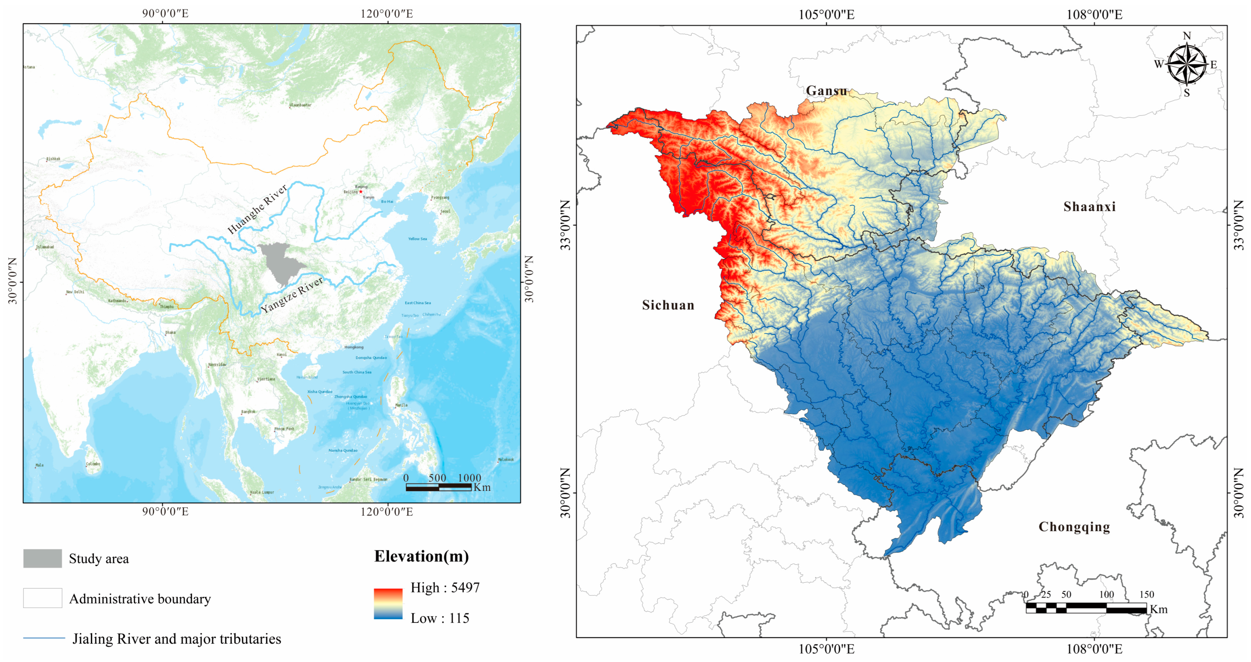
2. Overview of the Study Area

Geographically, the Jialing River basin is located between 102.55° E to 109.00° E and 29.67° N to 34.50° N, covering an area of approximately 160,000 km², spanning provinces such as Shaanxi, Sichuan, and Chongqing (Figure 1). The basin exhibits diverse topography, ranging from plateau to plain, with notable changes in altitude. Its climate falls under the humid subtropical type, characterized by abundant rainfall and moderate annual temperatures, making it a vital agricultural region suitable for cultivating crops such as rice, wheat, and maize, as well as being a primary area for economic crops such as rapeseed and cotton. Economically, the Jialing River basin is predominantly characterized by light industry and manufacturing, with rich mineral resources, especially coal, natural gas, and other energy minerals, which are essential in promoting economic growth. The Jialing River basin, with its unique geographical location, natural resources, and socio-economic factors, constitutes an important geographic unit in southwestern China.

3. Materials and Methods

The GlobeLand30 (2020) dataset, made available by the National Catalogue Service for Geographic Information (https://www.webmap.cn, accessed on 28 May 2024), is the primary source of LUCC data used in the research. The GlobeLand30 (2020) dataset is commonly used in LUCC investigations, with a resolution of 30 meters (overall accuracy = 0.8572, Kappa coefficient = 0.82). The land use statistics were classed into the following six categories: unused land, water area, forestland, construction land, farmland and grassland. Natural and societal causes are the main forces behind changes in land usage. The normalized difference vegetation index (NDVI), soil type, mean annual temperature, mean annual precipitation, and distance to rivers (found on https://www.webmap.cn, accessed on 28 May 2024), as well as the digital elevation model (DEM) and slope (calculated from the DEM) are the natural factors. The socioeconomic factors encompass the GDP density, population density (both sourced from https://www.resdc.cn, accessed on 28 May 2024), and the distances to railways, highways, first grade highways, secondary roads, tertiary roads, and county government (all sourced from https://www.webmap.cn, accessed on 28 May 2024). All these factors are processed into raster data with a 30-meter resolution.

The research methods mainly include the following elements (Figure 2):

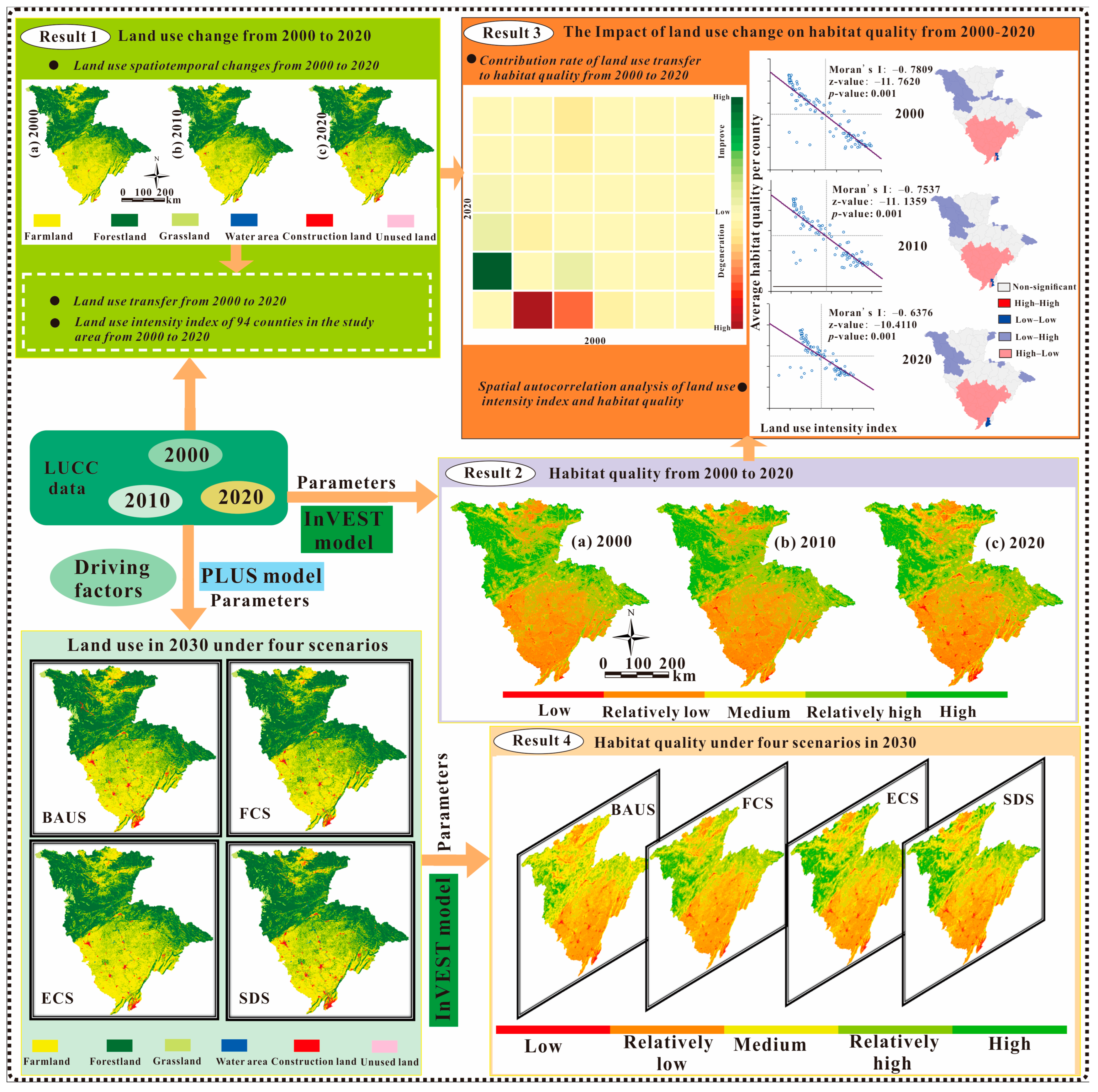
• the examination of the study area’s spatiotemporal variations in land use between the year 2000 and the year 2020 and calculating the land use intensity index for 94 counties;
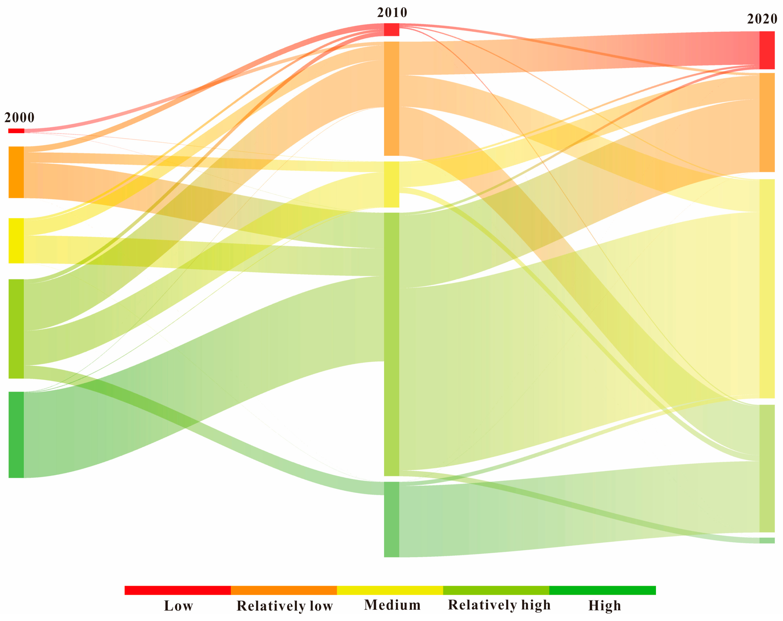
• the examination of the composition and geographic shifts in habitat quality between 2000 and 2020, taking notice of the distribution of habitat quality across various grades;
• the examination of LUCC’s effects on habitat quality during the years 2000 and 2020;
• the study and modeling of prospective habitat quality under four scenarios.

3.1. Analysis of Spatiotemporal Patterns of LUCC

3.1.1. Matrix of Land Use Transfer

An essential analytical tool for identifying patterns and trends in the conversion of various land types over time is a land use conversion matrix. This matrix measures the transitional links between distinct land types by comparing the changes in the geographical distribution of different land use categories at different intervals or times. This helps in understanding the evolution of land use patterns. The following formula may be used to get the land use conversion matrix:

$$A_{ij}=\left[\begin{array}{cccc}{A}_{11}& A_{12}& \cdots & A_{1n}\\ A_{21}& A_{22}& \cdots & A_{2n}\\ ⋮& ⋮& \ddots & ⋮\\ A_{n1}& A_{n2}& \cdots & A_{nn}\end{array}\right]$$

(1)

where A_ij represents the land area transferred from the beginning until the end of the era; i represents the kind of land use at the start of the era; j indicates the kind of land use at the end of the era; and n is the number of different forms of LUCC.

3.1.2. Land Use Intensity Index

The land use intensity index measures the variety and extent of land use in an area and serves as an indicator of the level of land development and use. This index typically integrates factors such as land use structure, intensity, and efficiency. The following is the formula for the land use intensity index:

$$L=100\times {\sum }_{i=1}^n{A}_i\times C_i$$

(2)

where L stands for the indicator of land use intensity; n is the number of different forms of land use; A_i stands for the land use category i intensity grading index (with values assigned as follows: unused land as 1, forestland, grassland, and water area as 2, farmland as 3, and construction land as 4 [31,32]); and C_i is the percentage of land that is used for land use category i.

3.2. PLUS Model and Multiple Scenario Setting

3.2.1. PLUS Model

The PLUS model is a powerful tool in the fields of landscape ecology and land use planning. The LEAS module and the CARS module make up the two main modules of the PLUS model [33]. To estimate the growth likelihood of different land categories, the LEAS module uses random sample sites, incorporates the LUCC driving elements, and applies the randomized forest classification method. In order to model future changes in land use, the CARS module is based on the initial land use circumstances and specifies important parameters such future demand for different property classes, a land conversion cost matrix, and neighborhood weights. The CARS module ensures limitations on the development likelihood of each land class while simulating the future state of land use through the creation of random seeds and a threshold decay mechanism. The integration of these two modules allows the PLUS model to not only provide a detailed analysis of land expansion but also forecast the future trends in land use [33].

Studies have shown that the PLUS model outperforms the FLUS model when it comes to modeling LUCC [33]. Jiang et al. found that the PLUS model produced the best results when comparing the simulation effects of the FLUS, CLUE-S, and PLUS models [34]. The PLUS model exhibited the best accuracy according to Lin and Peng’s simulations of future land use changes in the Fuxian Lake basin using the FLUS, CA–Markov, and PLUS model [35].

3.2.2. Model Evaluation

With the CARS module of the PLUS model, this study used land use data through 2000 and 2010 to estimate the geographical distribution of land use in 2020. Subsequently, the Kappa coefficient [36] and the overall accuracy were calculated based on simulated and actual data. Higher values indicate greater model performance. The Kappa coefficient and total accuracy have values between 0 and 1.

3.2.3. Future Scenario Setting

Given that Sichuan Province comprises the majority of the Jialing River basin, this study sets four scenarios for predicting the LUCC throughout the Jialing River basin for 2030, determined by the actual land use condition in the study region and by consulting the Sichuan Provincial Government’s papers on territorial spatial planning, natural resource preservation, and use. The following are the four possible future land use scenarios:

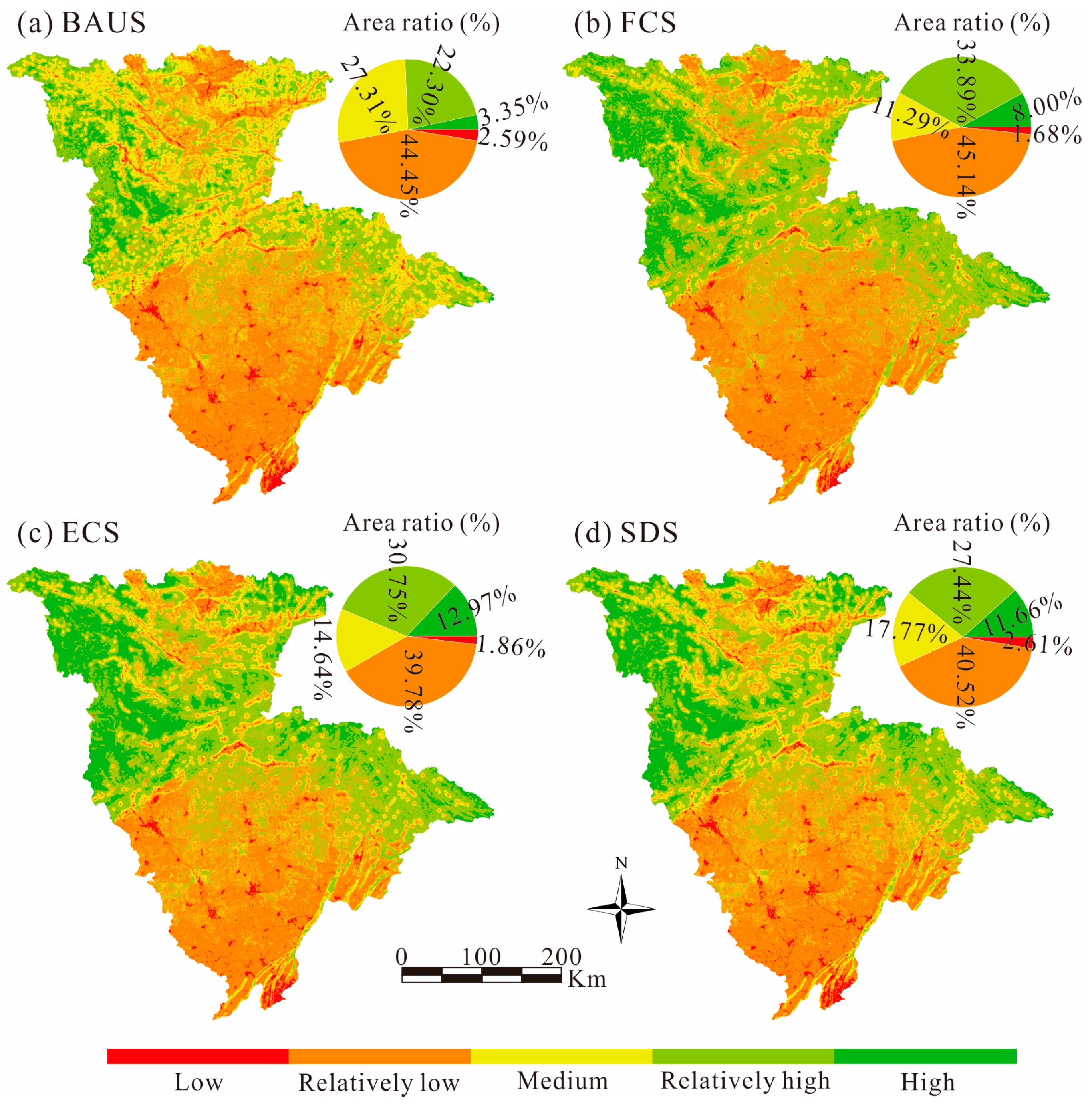
• The Business-as-usual Scenario (BAUS): This land use prediction for 2030 is based on changes in land use from 2010 to 2020, assuming that land use categories in the study region would vary from 2020 to 2030 according to historical trends and that there will not be any legislative restrictions on land use in 2030.
• The Farmland Conservation Scenario (FCS): Farmland protection is essential for food security since the studied region is a national agricultural producing region. Since it is forbidden to convert farmland to other land uses under the Farmland Conservation Scenario, there is a 20% increase in the likelihood of converting other land uses to farmland.
• The Ecological Conservation Scenario (ECS): The goal of ecological conservation is to coordinate land usage and ecological building in order to create a civilization that is favorable to the environment. In this scenario, converting forestland to other land types is prohibited, and the likelihood of water area and farmland being converted to construction or unused land is cut by 50%. Meanwhile, the probability of other land types being converted to forestland increases by 50%, while conversions to grassland and water area are elevated by 30%.
• The Sustainable Development Scenario (SDS): In response to the Chinese government’s initiatives to create a low-carbon, green economy, the preservation of the natural environment is given top priority throughout urban expansion, guaranteeing the long-term growth of the economy and society. There is a thirty percent rise in the likelihood of farmland being converted to forestland and grassland under the sustainable development scenario. There is an 80% decrease in the likelihood of converting forestland and grassland to farmland, and a 50% decrease in the likelihood of converting construction land to farmland. There is a 50% increased chance that unused land will be converted to construction land.

Setting the neighborhood weights, the land use demand for each type of land (

Table 1. The need for various land categories’ LUCC in 2030 throughout the four scenarios.

Scenarios	Land Use Demand (km2)
	Farmland	Forestland	Grassland	Water Area	Construction Land	Unused Land	Total
BAUS	65,258	84,263	6273	2059	3833	363	162,049
FCS	71,296	80,692	5753	1595	2398	315	162,049
ECS	61,293	90,365	5107	2059	3020	206	162,049
SDS	61,451	87,604	6708	2058	3865	365	162,049

), and the transition cost matrix (

Table 2. The transfer cost matrix under the four scenarios.

	BAUS						FCS						ECS						SDS
	A	B	C	D	E	F	A	B	C	D	E	F	A	B	C	D	E	F	A	B	C	D	E	F
A	1	1	1	1	1	1	1	0	0	0	0	0	1	1	1	1	1	1	1	1	1	1	1	1
B	1	1	1	1	1	1	1	1	1	0	1	1	0	1	1	1	1	0	1	1	1	1	1	1
C	1	1	1	1	1	1	1	1	1	1	1	1	0	1	1	1	1	0	1	1	1	1	1	1
D	1	1	1	1	1	1	1	0	1	1	0	0	0	0	0	1	0	0	0	0	0	1	1	0
E	1	1	1	1	1	1	1	1	1	1	1	1	1	1	1	1	1	1	1	0	1	0	1	0
F	1	1	1	1	1	1	1	1	1	1	1	1	1	1	1	1	1	1	1	1	1	1	1	1

Note: A, B, C, D, E, and F represent farmland, forestland, grassland, water area, construction land, and unused land, respectively. In this matrix, 1 represents conversion being possible, while 0 represents conversion not being possible.

) are necessary to predict foreseeable LUCC under all four scenarios in the CARS module. The transition cost matrix is based on historical experience [37,38], and the likelihood of transition for each scenario is used to compute the 2030 land need for each type. The neighborhood weights for unused land, water area, forestland, construction land, farmland and grassland are set at 0.58, 0.81, 0.53, 1, 0.1, and 0.58, respectively, according to the area of each land type’s growth.

3.3. InVEST Model and Habitat Quality Module

The InVEST model’s habitat quality module measures the appropriateness and degradation of habitats, helping users understand the impact of different land use types on biodiversity and ecosystem health [39]. This knowledge is essential for evaluating how human activity impacts ecosystem structure and function, particularly in the face of fast changes in land use and urbanization. Here is the formula to determine the quality of the habitat:

$$Q_{xj}=H_j[1-({\displaystyle \frac{D_{xj}^z}{D_{xj}^z+k^2}}\left)\right]$$

(3)

where Q_xj represents the habitat quality of raster x in land use type j, spanning 0 to 1, with lager values indicating better habitat quality; H_j is a representation of land use type j’s habitat appropriateness. D_xj represents the degree of habitat degradation; z is a constant used for normalization; and k, which is equal to half of the greatest deterioration degree, is the 50%-saturation parameter.

Setting the threat sources (

Table 3. The maximum impact distance, weight, and spatial attenuation type of the threat factors.

Threat Sources	Decay	Distance of Maximum Impact (km)	Weight
Unused land	Linear	4	0.4
Construction land	Exponential	9	0.9
Farmland	Linear	5	0.5

) and the sensitivity of various habitats (

Table 4. The habitat suitability and sensitivity to the threat factors for different land use types.

Land Use Type	Farmland	Forestland	Grassland	Water Area	Construction Land	Unused Land
Habitat suitability	0.3	0.9	0.7	0.75	0	0
Unused land	0.1	0.2	0.2	0.2	0	0
Construction land	0.6	0.6	0.5	0.8	0	0.2
Farmland	0	0.8	0.4	0.7	0	0

) to these threat variables is also required in order to compute D_xj. These two parameters were set up for this investigation based on the real conditions of the study location and on earlier research [24,40].

3.4. The Effect of LUCC on the Quality of Habitat

The habitat contribution rate is used to measure the habitat quality’s reaction to LUCC in order to make clear how changes in land use affect the quality of the habitat. The ratio of changes in habitat quality before and after changes in land use type is known as the habitat contribution rate. The following is the computing formula:

$$L_{ij=}\left(H_j-H_i\right){\displaystyle \frac{S_i}{S_t}}$$

(4)

where H_i and H_j stand for the habitat quality index of land use types i and j, respectively, and L_ij stands for the habitat contribution rate of the land use category i changing into j. The habitat quality indices in this study are set to 0.11, 0.54, 0.76, 0.18, 0.27, and 0.70 for unused land, water area, forestland, construction land, farmland, and grassland, respectively [40,41,42]. S_i and S_t stand for the area of land use category i changing into other land types and the study area as a whole, respectively.

3.5. Bivariate Examination of Spatial Autocorrelation

Spatial autocorrelation’s fundamental idea is that data values at close or adjacent places may show signs of resemblance or dependency. There are two categories of autocorrelation: local spatial autocorrelation and global spatial autocorrelation. These categories were employed to characterize the geographical heterogeneity of the local regions as well as the research area’s overall spatial distribution pattern [43,44,45]. The basic parameters in this analysis were each county’s average habitat quality and the land use degree index. In order to investigate the global and local spatial correlation between land use intensity and habitat quality, we used the bivariate spatial autocorrelation module in GeoDa (http://geodacenter.github.io/index-cn.html, accessed on 30 May 2024) to obtain the global Moran’s I index [46] and the local indicators of spatial association (LISA) maps [47].

4. Results

In this study, the LUCC data from 2000, 2010, and 2020 for the Jialing River basin were used to statistically analyze the area of each land use type and to employ a transition matrix, revealing the land use change characteristics in the study area over the past 20 years.

4.1. LUCC in the Jialing River Basin

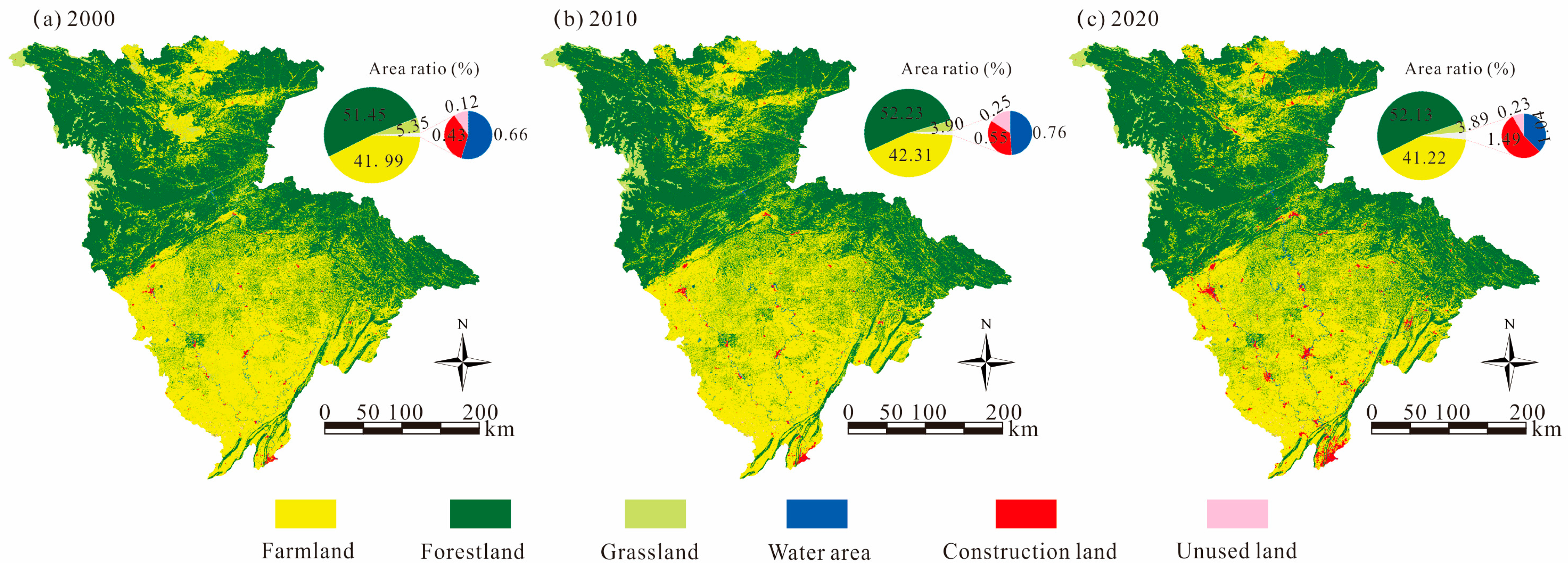
4.1.1. Spatial-Temporal Characteristics of LUCC between 2000 and 2020

The land use types in the Jialing River basin are primarily farmland and forestland, with other land types occupying relatively small areas. The distribution of farmland and forestland exhibits a clear north–south differentiation, with the farmland mainly distributed in the southern hilly areas and forestland predominantly distributed in the northern mountainous areas. The spatial distribution of most land types remained relatively stable between 2000 and 2020 (Figure 3), with the exception of construction land, which had minimal change between 2000 and 2010 but substantial expansion between 2010 and 2020 (Figure 3b,c).

Based on data regarding the area devoted to each form of land use between 2000 and 2020 (Figure 3,

Table 5. The area and proportion of six land use types from 2000 to 2020.

Year	Land Use Area (km2) and Proportion (%)
	Farmland	Forestland	Grassland	Water Area	Construction Land	Unused Land
2000	68,042 (41.99)	83,374 (51.45)	8663 (5.35)	1076 (0.66)	701 (0.43)	194 (0.12)
2010	68,558 (42.31)	84,640 (52.23)	6328 (3.90)	1233 (0.76)	891 (0.55)	399 (0.25)
2020	66,791 (41.22)	84,478 (52.13)	6300 (3.89)	1682 (1.04)	2424 (1.49)	374 (0.23)

), farmland has remained relatively stable, constituting almost 42% of the entire area, with an average area of approximately 67,797 km². With an average area of 84,164 km², the area of forestland has the largest proportion and has increased somewhat over the past 20 years, ranging between 51.45% and 52.13%. Over 90% of the entire area is made up of farming and forest land combined. Between 2000 and 2010, the grassland acreage shrank from 8663 km² to 6328 km², and remained essentially unchanged from 2010 to 2020. The water area continuously increased from 1076 km² in 2000 to 1682 km² in 2020, nearly doubling in size. The construction land area increased steadily over the 20-year period, with areas of 701 km² in 2000, 891 km² in 2010, and 2424 km² in 2020, showing a small increase from 2000 to 2010 and a significant increase by 2020. The area of unused land remained relatively small, with areas of 194 km², 399 km², and 374 km² in the three periods, respectively, showing an initial increase followed by stabilization.

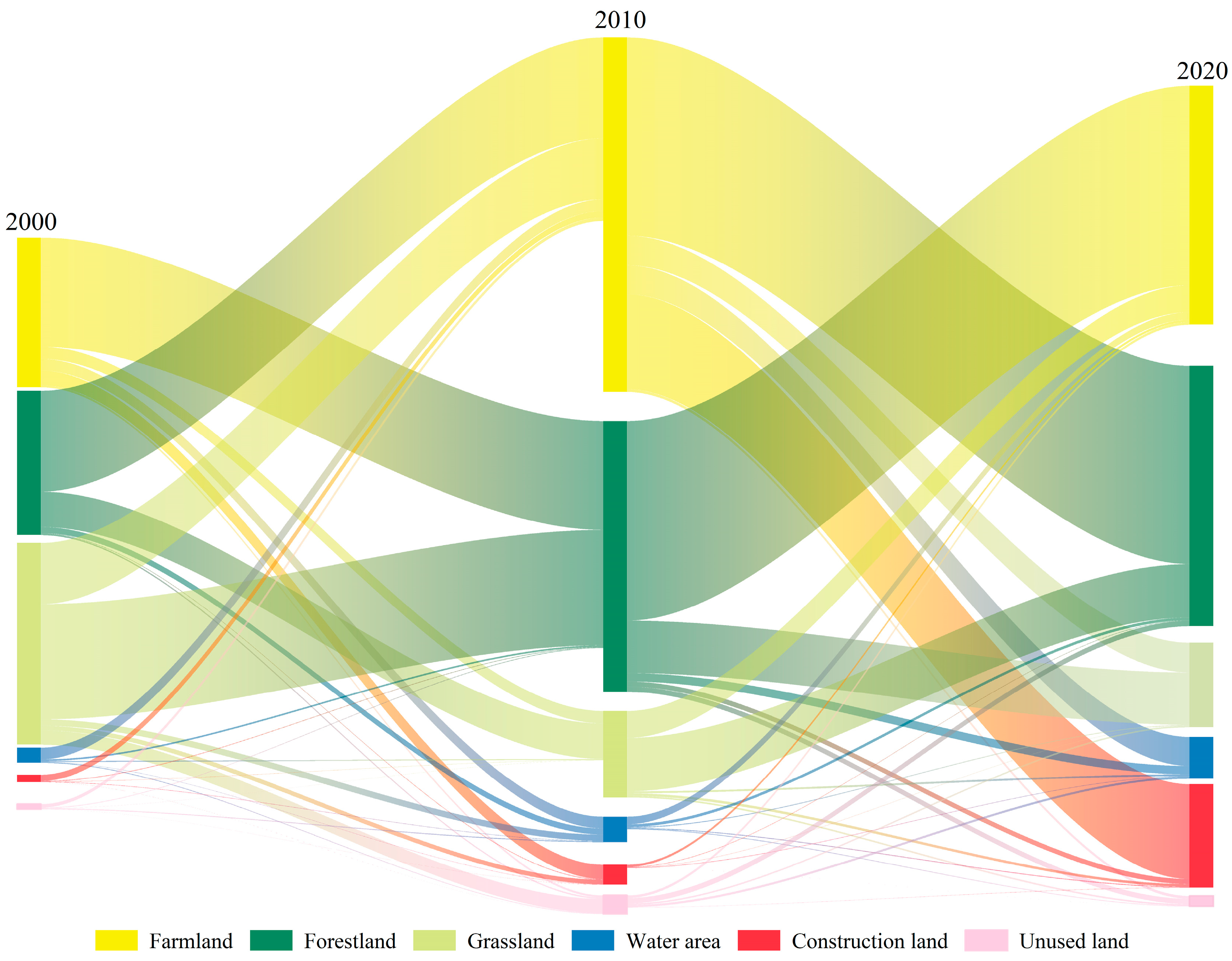
4.1.2. Land Use Transfer Analysis

Between 2000 and 2010, there were notable changes in the areas of farming, forestland, and grassland, as well as significant mutual conversions among these three land types. There was a net increase in the areas of water area, building land, and vacant land, respectively (

Table 6. The land use transfer areas between 2000 and 2020.

Year		2010
		A	B	C	D	E	F	Total
2000	A	65,749	1669	190	179	222	32	68,042
	B	1544	81,164	543	95	8	22	83,374
	C	935	1765	5575	97	71	219	8663
	D	179	25	14	844	3	10	1076
	E	97	8	4	6	585	1	701
	F	53	9	2	13	1	115	194
	Total	68,558	84,640	6328	1233	891	399	162,049
Year		2020
		A	B	C	D	E	F	Total
2010	A	63,131	3033	456	443	1452	43	68,558
	B	3057	80,492	801	129	79	81	84,640
	C	411	819	5004	29	39	25	6328
	D	116	43	12	1041	11	10	1233
	E	36	6	3	7	839	0	891
	F	40	84	24	33	4	215	399
	Total	66,791	84,478	6300	1682	2424	374	162,049

Note: Farmland, forests, grasslands, water area, construction land, and unutilized land are represented by the letters A, B, C, D, E, and F, in that order. Values represent km².

, Figure 4). During this period, farmland had an outgoing area of 2292 km², with 72.79% (1669 km²) converting to forestland. The incoming farmland area was 2809 km², mainly sourced from forestland and grassland, contributing 1544 km² and 935 km², respectively, and accounting together for 88.27% of the total incoming area (Table 6, Figure 4). The forestland’s departing area was 2292 km², of which 94.37% was made up of agriculture and grassland, with areas of 1544 km² and 543 km², respectively, after conversion. The incoming forestland area was 3476 km², mainly sourced from farmland and grassland, contributing 1668 km² and 1765 km², respectively, and together accounting for 98.78% of the total incoming area (Table 6, Figure 4). Of all land types combined, the grassland had the largest outgoing area, 3087 km², which was mostly converted to agriculture and forestland, with respective sizes of 935 km² and 1765 km², making up 87.46% of the overall outgoing area. The incoming grassland area was 752 km², mainly sourced from farmland and forestland, contributing 190 km² and 543 km², respectively, and together accounting for 97.44% of the total incoming area (Table 6, Figure 4). The water area was primarily converted to and from farmland, with a total conversion of 232 km², of which 179 km² was converted to farmland. The water area increased by 389 km², with farmland contributing 179 km². The conversions involving construction land and unused land also primarily occurred with farmland; the area of construction land decreased by 115 km² while expanding by 306 km², and unused land saw a reduction of 78 km² with an increase of 284 km².

The study area’s LUCC features from 2010 to 2020 mostly held steady with those from the decade before. Nonetheless, it is significant that the expansion of the land area used for building continued to grow (Table 6, Figure 4). A total of 5427 km² of farmland was moved out, mostly in favor of construction and forest land. Of this total, 82.64% of the transfer-out area was made up of 3033 km² and 1452 km² of transfer-out areas, respectively. A total of 3660 km² of farmland was transferred in, primarily from forestland, which accounted for 3057 km², or 83.53%, of the entire area transferred in (Table 6, Figure 4). The forestland transferred out amounted to 4147 km², mainly for farmland and grassland, with transfer-out areas of 3057 km² and 801 km², respectively, accounting for 93.03% of the total transfer-in area. The area of forestland transferred in was 3985 km², primarily from farmland and grassland, which contributed 3033 km² and 819 km², respectively, accounting for 89.13% of the total transfer-in area (Table 6, Figure 4). The grassland transferred out amounted to 1323 km², mainly to farmland and forestland, with transfer-out areas of 411 km² and 819 km², respectively, accounting for 92.99% of the total transfer-out area. The area of grassland transferred in was 1295 km², mainly from farmland and forestland, which contributed 456 km² and 801 km², respectively, accounting for 97.00% of the total transfer-in area (Table 6, Figure 4). The transfers in and out of the water area primarily occurred with farmland, with transfer-out and transfer-in areas of 192 km² and 641 km², respectively, including 12 km² from water area to farmland and 443 km² from farmland to water area. The change in construction land was significant, with a transfer-out area of 52 km² and a transfer-in area of 1585 km², of which farmland contributed 1452 km². The transfers in and out of unused land mainly occurred with forestland, maintaining a relatively balanced area (Table 6, Figure 4).

Farmland, forestland, and grassland have all seen significant area changes over the last 20 years due to active mutual conversions between the three types. The areas of water area and construction land saw the most transfers, particularly between 2010 and 2022, when a substantial portion of farmland was turned into construction land. This resulted in a notable increase in the area of construction land relative to the preceding decade, perhaps as a result of the recent ten years’ rapid urbanization. Overall, the amount of unused land showed a certain degree of increase.

4.2. Patterns of Temporal and Spatial Evolution in Habitat Quality

The geographic distributions of habitat quality for the years 2000, 2010, and 2020 were produced by entering the pertinent parameters into the InVEST model’s habitat quality. Throughout the research region for these years, the habitat quality values varied around 0 to 0.9, with average values of 0.5401, 0.5338, and 0.5084. This indicates a high local habitat structure and landscape stability, relatively rich species diversity, but overall moderate habitat quality, significantly impacted by human activities [48]. Furthermore, the habitat quality exhibited a gradual decline from 2000 to 2020, with more pronounced deterioration from 2010 to 2020.

The habitat quality for 2000, 2010, and 2020 was categorized into five categories, from low [0~0.2), relatively low [0.2~0.4), medium [0.4~0.6), to relatively high [0.6~0.8), and high [0.8~0.9). Spatially, the study area exhibits a southern–northern gradient in habitat quality, with a higher overall habitat quality observed in the northern regions compared to the southern regions (Figure 5). The northern areas predominantly have relatively high- and high-quality habitats, followed by relatively low-quality habitats. In contrast, the southern regions primarily have relatively low-quality habitats. Furthermore, most of the areas designated as high-quality habitats are found in the northern sections, whereas the majority of the areas designated as low-quality habitats are found in the southern sections.

According to the habitat quality levels from low to high, the areas in 2000 were 894 km², 68,531 km², 8414 km², 55,158 km², and 29,053 km², corresponding to proportions of 0.55%, 42.29%, 5.19%, 34.04%, and 17.93%, respectively. In 2010, the areas were 1291 km², 69,166 km², 8454 km², 57,424 km², and 25,715 km², corresponding to proportions of 0.80%, 42.68%, 5.22%, 35.43%, and 15.87%, respectively. In 2020, the areas were 2798 km², 68,481 km², 17,043 km², 51,205 km², and 22,523 km², with proportions of 1.72%, 42.26%, 10.52%, 31.60%, and 13.90%, respectively (

Table 7. The habitat quality domain for all levels between 2000 and 2020.

Year	Area (km2)
	Low	Relatively Low	Medium	Relatively High	High
2000	894	68,531	8414	55,158	29,053
2010	1291	69,166	8454	57,424	25,715
2022	2798	68,481	17,043	51,205	22,523

). These statistics show that throughout the course of the 20-year period, the habitat quality shows the following patterns: (1) the areas with low-quality habitats expand annually, while those with high-quality habitats shrink, creating a distinct contrast between the two; (2) the regions with both low and high habitat quality first expand and then contract, with overall variations being relatively modest; and (3) the regions with medium-quality habitat expand annually, with more pronounced growth in the latter decade compared to the first decade.

From the perspective of the habitat area transitions (

Table 8. The shift in habitat quality between 2000 and 2020.

Year		2010
		A	B	C	D	E	Total
2000	A	703	166	17	9	0	894
	B	268	66,164	473	1625	1	68,531
	C	119	672	6345	1272	6	8414
	D	200	2147	1589	50,620	602	55,158
	E	1	18	29	3899	25,106	29,053
Year		2020
		A	B	C	D	E	Total
2010	A	1058	116	55	60	1	1291
	B	1528	63,940	1446	2249	2	69,166
	C	90	1086	7008	269	0	8454
	D	120	3333	8348	45,360	263	57,424
	E	2	5	186	3266	22,258	25,715

Note: The following habitat quality classes are represented by the letters A, B, C, D, and E: A denotes low, B relatively low, C denotes medium, D relatively high, and E denotes high. Values presented in km².

, Figure 6), from 2000 to 2010, the low-quality habitat areas saw an outflow of 192 km², of which 166 km² transitioned to relatively low-quality habitats; additionally, the inflow into low-quality habitats was 588 km², with almost no inflow from high-quality habitats. The relatively low-quality habitats collectively saw an outflow of 2367 km², primarily transitioning to relatively high-quality habitats, amounting to 1625 km²; the inflow into relatively low-quality habitats was 3002 km², with contributions mainly from relatively high-quality habitats totaling 2147 km², followed by medium-quality habitats. The medium-quality habitats had an outflow of 2068.57 km², primarily transitioning to relatively high-quality habitats (1272 km²), followed by relatively low-quality habitats; the inflow into medium-quality habitats was 2108.12 km², with contributions mainly from relatively high-quality habitats amounting to 1588.74 km². The relatively high-quality habitats had an outflow of 4537 km², primarily transitioning to either the relatively low-quality habitats or upgrading to medium-quality habitats, with outflows of 2147 km² and 1589 km², respectively; the inflow into the relatively high-quality habitats was 6804.53 km², with contributions of 3899 km² from the high-quality habitats. The high-quality habitats had an outflow of 3947 km², predominantly transitioning to relatively high-quality habitats; the inflow into the high-quality habitats was 609 km², almost entirely from the relatively high-quality habitats.

From 2010 to 2020, on examining the habitat quality transitions using each grade in turn (Table 8, Figure 6), the low-quality habitats saw an outflow of 233 km², of which 116 km² transitioned to relatively low-quality habitats, with the remainder split between relatively low-quality and medium-quality habitats, and with very little inflow from high-quality upgrades; the inflow into low-quality habitats was 1740 km², primarily from relatively low-quality habitats, with almost no inflow from high-quality habitats. The relatively low-quality habitats collectively saw an outflow of 5225 km², primarily transitioning to relatively high-quality habitats (2249 km²), followed by low-quality and medium-quality habitats; the inflow into relatively low-quality habitats was 4540 km², with contributions mainly from the relatively high-quality habitats amounting to 3333 km², followed by the medium-quality habitats. The medium-quality habitats had an outflow of 1446 km², primarily transitioning to relatively low-quality habitats (1086 km²); the inflow into medium-quality habitats was 10,035 km², with contributions mainly from the relatively high-quality habitats amounting to 8348 km². The relatively high-quality habitats had an outflow of 12,064 km², primarily transitioning to medium-quality habitats and upgrading from relatively low-quality habitats, with outflows of 8348 km² and 3333 km², respectively; the inflow into relatively high-quality habitats was 5844 km², with contributions of 3266 km² from the high-quality habitats and 2249 km² from the relatively low-quality habitats. Finally, the high-quality habitats had an outflow of 3458 km², predominantly transitioning to relatively high-quality habitats; the inflow into high-quality habitats was 266 km², almost entirely from relatively high-quality habitats.

The primary cause of the diminishing habitat quality is clearly the considerable transfer of relatively high-quality habitats to those habitats outside the high-quality categories, as shown by the comparative assessments of the habitat grade changes over the previous 20 years. Additionally, the more pronounced decline in overall habitat quality over the last 10 years is primarily due to a much larger area of degradation in the relatively high-quality habitats compared to the previous 10 years.

4.3. Changes in Land Use’s Effects on Habitat Quality

4.3.1. Land Use Transfer’s Effect on Habitat Quality

Depending on the types of land use involved, land use transformations have various effects on the quality of the environment. Overall, the quality of the habitat was only slightly impacted by the majority of land use changes in this research region (Figure 7). Farmland modification, which is strongly related to the relative area of each land type, is the main cause of changes in habitat quality. Transforming farmland into forestland leads to the greatest enhancement in habitat quality, followed by the conversion of farmland to grassland, and grassland to forestland. Conversely, the conversion of forestland to farmland and grassland to farmland substantially degrades the habitat quality, followed by transitions from grassland to unused land, grassland to construction land, water area to farmland, and forestland to grassland (Figure 7).

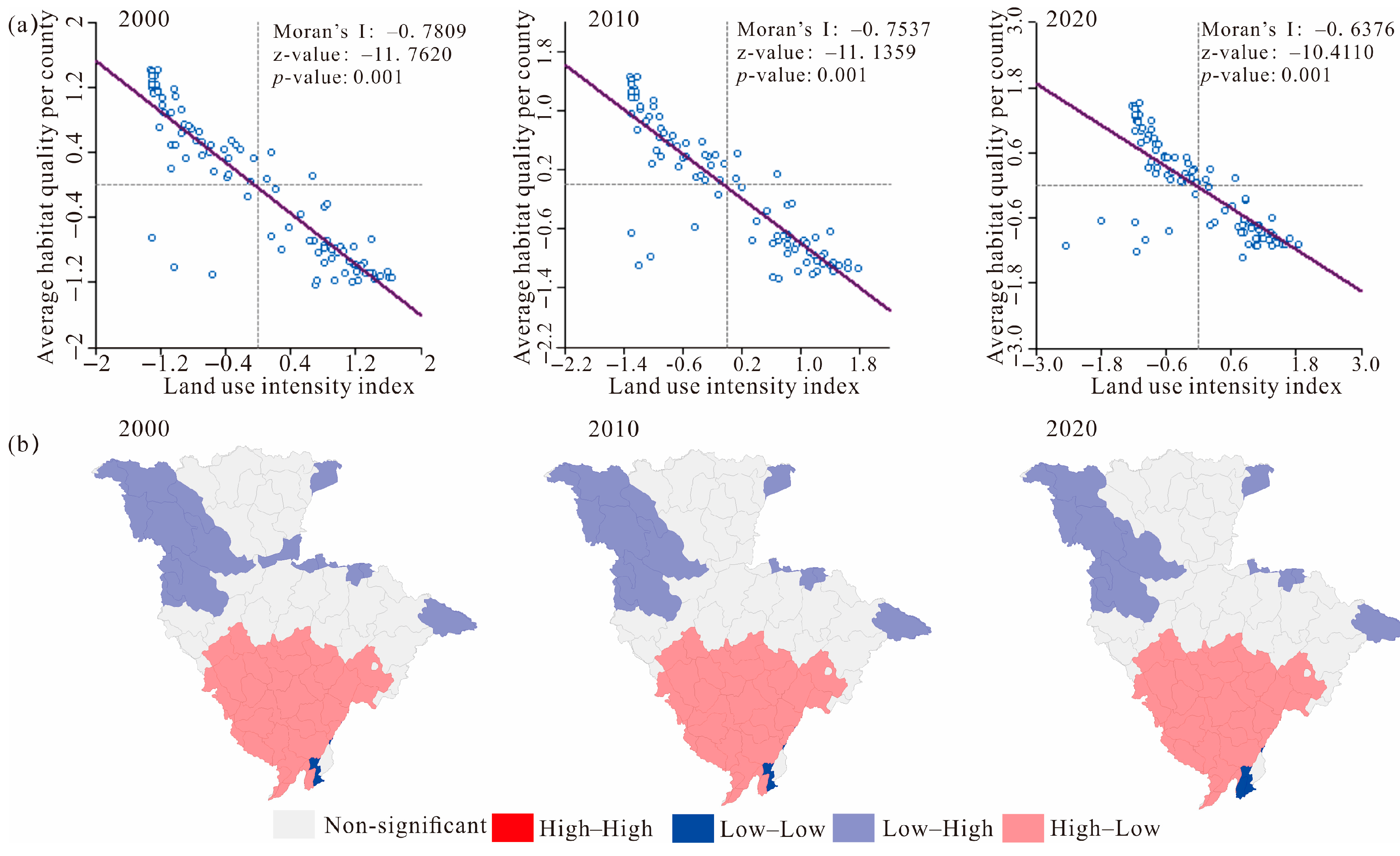
4.3.2. The Association between Habitat Quality and Land Use Intensity

A study was carried out at the county level to look at the local and global connections between the land use intensity indices and habitat quality in order to learn more about the effects of land use change on habitat quality. Using GeoDa software with 999 iterations, the global Moran’s I indices for the years 2000, 2010, and 2022 were calculated as −0.7809, −0.7537, and −0.6376, respectively. The corresponding p-values were 0.001, and the z-values were −11.7620, −11.1259, and −10.4110 (Figure 8a). With a confidence level higher than 99%, these data show a substantial inverse relationship between the study area’s land use intensity and habitat quality.

The analysis of the global Moran’s I indices over the three periods shows a trend of gradual decrease followed by a steep decline, suggesting a reduction in spatial heterogeneity over time. This pattern suggests that habitat quality tends to decline with increasing land use intensity as well as vice versa.

The LISA map visualizes significant spatial correlations between the different areas within the study region. In the Jialing River basin, two main patterns are observed, high–low and low–low. Throughout 2000 to 2020, the high–low pattern’s geographical distribution remained mostly constant, with the majority of its concentration occurring in the southern portion of the research region (Figure 8b). This pattern shows the locations where low habitat quality is correlated with high land use intensity. In the study region’s eastern and northwest margins, the low–low pattern is visible. From 2000 to 2020, this pattern showed a gradual decrease in spatial distribution, although the reduction in extent was minimal.

4.4. Multi-Scenario Modeling and Habitat Quality Analysis

After comparing the simulated land use data for 2020 with the real land use data, the PLUS model’s CARS module produced a Kappa coefficient of 0.8579 and an overall accuracy of 0.922076. These indicators show that the PLUS model simulates future land changes in the study region with a high degree of accuracy. Land use statistics for 2030 were simulated under four different scenarios using the PLUS model. These scenarios were combined with the actual 2020 land use data to assess the habitat quality in 2030 using the habitat quality module of the InVEST model (Figure 9). Under the BAUS, FCS, ECS, and SDS, the research area’s average habitat quality was, in turn, 0.4381, 0.4940, 0.5123, and 0.4908, respectively. Under the ECS, the habitat quality only slightly improved as compared to 2020; in contrast, under the other scenarios, it declined to varied degrees.

Under the BAUS in 2030, the proportions of habitat quality levels (the same as 2000–2020) were as follows: 2.59% (low), 44.45% (relatively low), 27.31% (medium), 22.30% (relatively high), and 3.35% (high). Compared to 2020, the changes were +0.87%, +2.19%, +16.79%, −9.30%, and −10.55%, respectively. Under the FCS in 2030, the proportions were as follows: 1.68% (low), 45.14% (relatively low), 11.29% (medium), 33.89% (relatively high), and 8.00% (high). The changes compared to 2020 were −0.04%, +2.88%, +0.77%, +2.29%, and −5.90%. Under the ECS in 2030, the following proportions were obtained: 1.86% (low), 39.78% (relatively low), 14.64% (medium), 30.75% (relatively high), and 12.97% (high). The changes compared to 2020 were +0.14%, −2.48%, +4.12%, −0.85%, and −0.93%. Under the SDS in 2030, the following proportions were obtained: 2.61% (low), 40.52% (relatively low), 17.77% (medium), 27.44% (relatively high), and 11.66% (high). The changes compared to 2020 were +0.89%, −1.74%, +7.25%, −4.16%, and −2.24%.

Under the BAUS from 2020 to 2030, the area starting with a relatively high habitat quality that transitioned to a medium habitat quality was the largest at 26,185 km². Next, the transition area of the high-quality habitats to relatively high-quality habitats totaled 12,882 km², while there was almost no transition into high-quality habitats (Figure 10a). Under the FCS, the largest transition area was from the high-quality habitats to relatively high-quality habitats (9331 km²), followed by transitions from relatively high-quality and medium-quality habitats to medium-quality habitats (2869 km²) and relatively low-quality habitats (2804 km²). The transition into the low- and high-quality habitats was minimal (Figure 10b). Under the ECS, there was a significant decrease in the area of high-quality habitats transitioning out, with substantial reductions in the transitions to relatively high-quality habitats and into low-quality habitats (Figure 10c). Under the SDS, the most significant transition area was from the relatively high-quality habitats to medium-quality habitats (11,205 km²), followed by transitions from high-quality habitats to relatively high-quality habitats (3519 km²). There was almost no transition into the high-quality habitats, but there was a notable increase in transitions from the relatively low-quality habitats to low-quality habitats (1458 km²) (Figure 10d).

5. Discussion

5.1. LUCC’s Effects on the Quality of the Habitat

This study revealed the spatiotemporal patterns in different land use types and their possible effects on the local ecosystems by examining the land use changes in the Jialing River basin and their implications for habitat quality. From 2000 to 2020, the study area’s land use distribution revealed that farming predominated in the south and forestland in the north. Over this 20-year period, the most notable changes were a 1.46% decrease in grassland and a 1.07% increase in construction land, aligning with previous research findings [49].

From 2000 to 2020, the Jialing River basin’s northern portion had higher habitat quality than its southern portion, consistent with the findings of Du and Qu [50]. According to Yang et al.’s study, the Sichuan basin’s habitat quality for the years 2000, 2010, and 2020 was 0.4579, 0.4585, and 0.4622, respectively [51]. These values are slightly lower than our findings, and the trend in habitat quality changes is the opposite to ours. There are two main reasons for this. First, the Sichuan basin includes the Chengdu–Chongqing economic circle, which is a significant factor leading to the overall lower habitat quality compared to the Jialing River basin. Second, although there are overlapping areas between the Sichuan basin and the Jialing River basin, they are not entirely the same. Therefore, the habitat quality between the two regions is slightly different, and the change trends are inconsistent. In the eastern portion of the Jialing River basin, the Three Gorges reservoir region (Chongqing section) was the subject of a study by Liang et al. The findings indicated that the habitat quality values for the years 2000, 2010, and 2020 were 0.502, 0.507, and 0.499, respectively [40]. Due to the similar natural and economic conditions in both regions, these habitat quality values are relatively consistent. Liang et al. also indicated that the main land use change type that promoted regional habitat quality improvement from 2000 to 2020 was the conversion of farmland to forestland and grassland; meanwhile, the main land use change type that led to habitat quality degradation was the conversion of grassland and forestland to farmland [40]. These outcomes completely agree with what we discovered. Similar results have been observed in Ethiopia [27], a region with relative economic poverty. In places with higher levels of economic development, such as Wuxi, China [52] and the Guangdong–Hong Kong–Macao Greater Bay Area [53], the increase in construction land areas and the decrease in cultivated land areas are the main causes of habitat quality degradation.

The findings highlight the significant alterations in the study area’s land use patterns over the past two decades, particularly the pronounced habitat fragmentation and degradation resulting from the encroachment of farmland into forestland and grassland (Figure 7). Due to the expansion of farmland, the connectivity between the patches is inhibited, thereby significantly exacerbating the habitat fragmentation and degradation [27,54,55,56]. This phenomenon is a direct outcome of both changes in the land use pattern and the serious problems that ecosystem services and biodiversity are confronting. Taking Malaysia and Indonesia as examples, the extensive expansion of oil palm plantations has led to vast reductions in forest cover, triggering serious issues in ecosystem function restoration and habitat connectivity [54]. Studies have shown that the effects of increasing farmland on the structure and function of ecosystems go beyond simple changes in land size, having a substantial impact on local climate, carbon storage, soil quality, and water resource management [57,58,59,60,61]. Recent academic research has underscored the multifaceted impacts of farmland expansion on both ecosystems and socio-economics. For instance, China’s rapid agricultural modernization process has significantly altered land use patterns, exacerbating the fragmentation and degradation of natural ecosystems like grassland and forestland [62,63,64]. These modifications have not only had a significant effect on the composition and operation of nearby ecosystems, but they have also made the reduction in ecosystem services and biodiversity loss worse [54].

5.2. Challenges and Strategies for Future Habitats

Using numerous scenario simulations, this study forecasts developments in habitat quality in the Jialing River basin under various land use scenarios. The simulation results indicate that if the current land use patterns continue (i.e., BAUS), habitat quality will deteriorate further, especially in those areas with intensive agricultural activities. Under the FCS and SDS, agricultural expansion and urbanization will continue to encroach upon natural habitats, exacerbating habitat fragmentation and decreasing the ecosystem service functions. Conversely, under the ECS, enhancing ecological protection and restoration measures, such as increasing the forest cover and restoring degraded water area, can effectively improve habitat quality and enhance ecosystem service functions, providing clear directions for regional ecological environment management.

We consult pertinent government documents and integrate the results of this investigation with our recommendations for habitat enhancement in order to address the threats that the habitat in the research region faces. Local governments throughout the Jialing River basin should adopt measures such as reforestation, converting farmland to forests and grasslands, and transforming unsuitable farmland (e.g., sloping land over 25 degrees, severely desertified areas) into forests and grasslands, in line with the basin’s ecological function zoning. Land use control policies should be strictly enforced, the illegal occupation of forests and grasslands for agricultural reclamation should be prohibited, and the approval process for land use changes should be strengthened to ensure that land use aligns with ecological protection requirements. In concentrated agricultural areas, eco-friendly agricultural technologies should be encouraged to minimize environmental degradation and promote the growth of green agriculture. Additionally, by utilizing the resources already available in the forest and grasslands, eco-tourism should be developed and local economic growth should be supported while ecological preservation is preserved.

5.3. Study Limitations and Potential for the Future

There are several limitations to this work, despite its thorough examination of how changes in land use affect the habitat quality in the Jialing River basin through the use of ecological models and remote sensing technologies. Firstly, due to data accessibility issues, this study utilized the GlobeLand30 (2020) dataset without comparing its interpretative accuracy to other paid datasets, such as CNLUCC. The study’s accuracy may be affected by the land use data’s spatial resolution and interpretation accuracy, as higher resolution and accuracy make it easier to use the PLUS model to forecast changes in land use in the future and the InVEST model to calculate habitat quality under various scenarios. Secondly, this study heavily relied on existing ecological models and remote sensing data, which may lack detailed descriptions and explanations of microhabitat changes. Moreover, some model parameters are often based on previous experiences, adding uncertainty to the results. For instance, the transfer cost matrix used in the PLUS model for future land use predictions and the threat sources and sensitivity required for calculating habitat quality using the InVEST model are all based on previous studies. Specifically, in calculating the habitat quality through the InVEST model, we referred to the experiences of Li [24] and Liang [40] for setting the threat sources and sensitivity, as their study areas were close to the Jialing River basin. The manual setting of threat sources and sensitivity is a significant source of uncertainty in calculating habitat quality using the InVEST model. This uncertainty arises mainly from the two following factors: (1) these parameters are primarily set based on previous experience, without considering whether the parameters are region-specific, raising doubts about their suitability for the current study area; and (2) in studying the habitat quality over a specific period, a single set of parameters is often used across multiple time points, raising the question of whether the parameters (such as maximum impact distance, influence weight, etc.) should vary over time.

To address these issues, future research could be improved with the use of higher resolution technologies and more accurate land use data to enhance the precision and reliability of the findings. Additionally, combining field surveys to determine the optimal parameter combinations required for the models would be beneficial. Furthermore, this study only qualitatively examined the reasons for changes in habitat quality in the Jialing River basin from the standpoint of land use changes due to the constraints of the InVEST model. Nevertheless, other factors could also have an impact on changes in habitat quality, indicating that more thorough study from a variety of angles should be conducted in the future.

6. Conclusions

This study evaluated the Jialing River basin’s habitat quality from 2000 to 2020 based on changes in land use, and it coupled the PLUS and InVEST models to provide multi-scenario simulations of the habitat quality in the future. The following are the primary conclusions:

• In the study area, the southern hilly regions are primarily covered with farmland, while the northern mountainous regions are predominantly forested. Together, these two land types constitute over 90% of the area’s total land cover. Over the past 20 years, the most significant changes in land type proportions include a decrease of 1.46% in grassland and an increase of 1.07% in construction land. The expansion of construction land was particularly pronounced in the latter 10 years compared to the earlier decade.
• The research area’s habitat quality value range for the years 2000, 2010, and 2020 was 0 to 0.9, with corresponding average values of 0.5401, 0.5338, and 0.5084. This indicates that overall habitat quality is typically modest with a danger of additional decline, even while small regions show a high habitat structure and landscape stability.
• The habitat quality of the study region is directly correlated with the percentage of each land use type, and most land use changes have a negligible effect on it. The main factor contributing to the deterioration of habitat quality is farmland’s encroachment into grasslands and forests.
• With a tendency towards declining spatial heterogeneity, the worldwide Moran’s I indices for the years 2000, 2010, and 2022 were −0.7809, −0.7537, and −0.6376, respectively, showing a substantial negative association between land use intensity and habitat quality in the studied region. The research region mostly displays the following two modes, according to the LISA maps: high land use intensity related to poor habitat quality (high–low) and low land use intensity relating to low habitat quality (low–low).
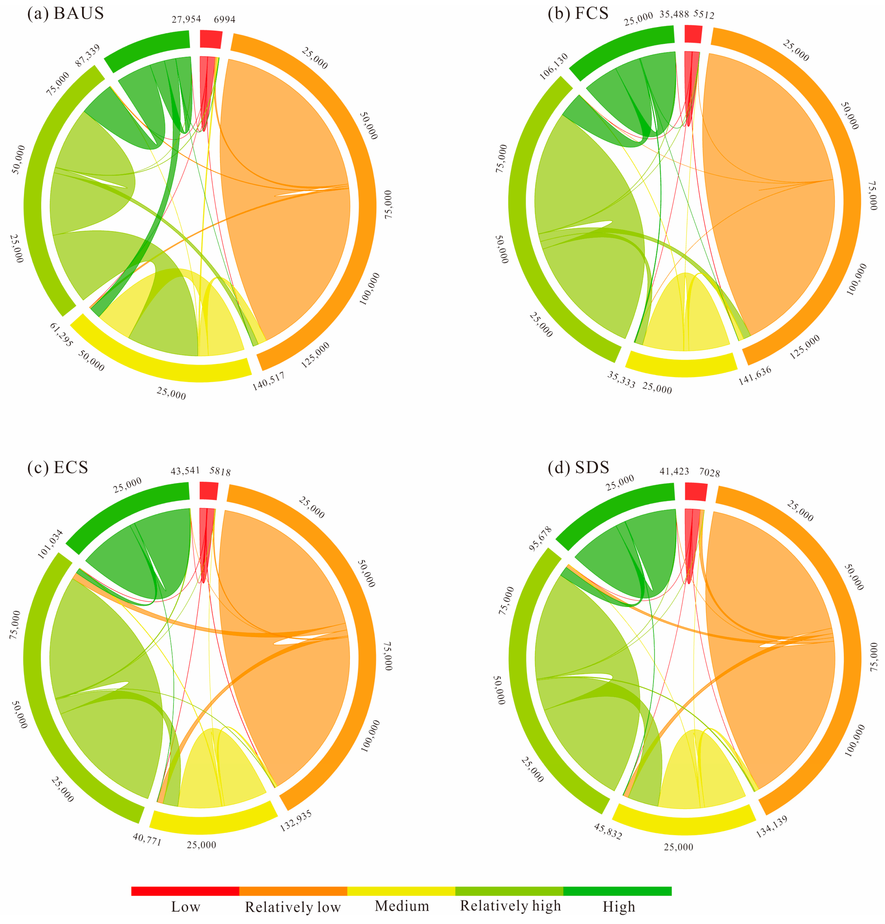
• The results of the habitat simulations under the four future scenarios show that, with the exception of the ecological protection scenario, where habitat quality improves, there is a specific level of degradation in the habitat quality under the business-as-usual, farmland conservation, and sustainable development scenario. Active ecological protection measures have a significant effect on improving habitat quality, providing a clear direction for ecological environment management in the study area.

The manual setup of the model parameters was the main source of this study’s shortcoming. Any future research can improve the accuracy by conducting field investigations to obtain an optimal set of parameters. Furthermore, the Jialing River basin’s habitat quality changes were solely examined qualitatively in this study from the standpoint of land use change. Subsequent research endeavors may conduct a more comprehensive analysis of the alterations in habitat quality by taking into account various viewpoints.

References

1. Bunce, R.G.H.; Bogers, M.M.B.; Evans, D.; Halada, L.; Mucher, S.; Bauch, B.; De Blust, G.; Parr, T.W.; Olsvig-Whittaker, L. The significance of habitats as indicators of biodiversity and their links to species. Ecol. Indic. 2012, 33, 19–25. [Google Scholar] [CrossRef]
2. Petren, K. Habitat and Niche, Concept of. In Encyclopedia of Biodiversity, 2nd, ed.; Levin, S.A., Ed.; Academic Press: Waltham, MA, USA, 2001; pp. 39–49. [Google Scholar]
3. Doi, H.; Katano, I.; Negishi, J.N.; Sanada, S.; Kayaba, Y. Effects of biodiversity, habitat structure, and water quality on recreational use of rivers. Ecosphere 2013, 4, art102. [Google Scholar] [CrossRef]
4. Cardinale, B.J.; Duffy, J.E.; Gonzalez, A.; Hooper, D.U.; Perrings, C.; Venail, P.; Narwani, A.; Mace, G.M.; Tilman, D.; Wardle, D.A.; et al. Biodiversity loss and its impact on humanity. Nature 2012, 486, 59–67. [Google Scholar] [CrossRef] [PubMed]
5. Fahrig, L. Effects of Habitat Fragmentation on Biodiversity. Annu. Rev. Ecol. Evol. Syst. 2003, 34, 487–515. [Google Scholar] [CrossRef]
6. Marselle, M.R.; Lindley, S.J.; Cook, P.A.; Bonn, A. Biodiversity and Health in the Urban Environment. Curr. Environ. Health Rep. 2021, 8, 146–156. [Google Scholar] [CrossRef]
7. Heinz, A.; Deserno, L.; Reininghaus, U. Urbanicity, social adversity and psychosis. World Psychiatry Off. J. World Psychiatr. Assoc. (WPA) 2013, 12, 187–197. [Google Scholar] [CrossRef]
8. McDonald, R.I.; Mansur, A.V.; Ascensão, F.; Colbert, M.L.; Crossman, K.; Elmqvist, T.; Gonzalez, A.; Güneralp, B.; Haase, D.; Hamann, M.; et al. Research gaps in knowledge of the impact of urban growth on biodiversity. Nat. Sustain. 2020, 3, 16–24. [Google Scholar] [CrossRef]
9. Liu, D.; Liang, X.; Chen, H.; Zhang, H.; Mao, N. A Quantitative Assessment of Comprehensive Ecological Risk for a Loess Erosion Gully: A Case Study of Dujiashi Gully, Northern Shaanxi Province, China. Sustainability 2018, 10, 3239. [Google Scholar] [CrossRef]
10. Gao, Y.; Ma, L.; Liu, J.; Zhuang, Z.; Huang, Q.; Li, M. Constructing Ecological Networks Based on Habitat Quality Assessment: A Case Study of Changzhou, China. Sci. Rep. 2017, 7, 46073. [Google Scholar] [CrossRef]
11. Nelson, E.; Mendoza, G.; Regetz, J.; Polasky, S.; Tallis, H.; Cameron, D.; Chan, K.M.A.; Daily, G.C.; Goldstein, J.; Kareiva, P.M.; et al. Modeling multiple ecosystem services, biodiversity conservation, commodity production, and tradeoffs at landscape scales. Front. Ecol. Environ. 2009, 7, 4–11. [Google Scholar] [CrossRef]
12. Polasky, S.; Nelson, E.; Pennington, D.; Johnson, K.A. The Impact of Land-Use Change on Ecosystem Services, Biodiversity and Returns to Landowners: A Case Study in the State of Minnesota. Environ. Resour. Econ. 2011, 48, 219–242. [Google Scholar] [CrossRef]
13. McKinney, M. Urbanization, Biodiversity, and Conservation. BioScience 2002, 52, 883–890. [Google Scholar] [CrossRef]
14. McDonald, R.I.; Kareiva, P.; Forman, R.T.T. The implications of current and future urbanization for global protected areas and biodiversity conservation. Biol. Conserv. 2008, 141, 1695–1703. [Google Scholar] [CrossRef]
15. Kowarik, I. Novel urban ecosystems, biodiversity, and conservation. Environ. Pollut. 2011, 159, 1974–1983. [Google Scholar] [CrossRef] [PubMed]
16. Güneralp, B.; Lwasa, S.; Masundire, H.; Parnell, S.; Seto, K.C. Urbanization in Africa: Challenges and opportunities for conservation. Environ. Res. Lett. 2017, 13, 015002. [Google Scholar] [CrossRef]
17. Haddad, N.M.; Brudvig, L.A.; Clobert, J.; Davies, K.F.; Gonzalez, A.; Holt, R.D.; Lovejoy, T.E.; Sexton, J.O.; Austin, M.P.; Collins, C.D.; et al. Habitat fragmentation and its lasting impact on Earth’s ecosystems. Sci. Adv. 2015, 1, e1500052. [Google Scholar] [CrossRef]
18. Li, X.; Yeh, A.G.-O. Analyzing spatial restructuring of land use patterns in a fast growing region using remote sensing and GIS. Landsc. Urban Plan. 2004, 69, 335–354. [Google Scholar] [CrossRef]
19. Seto, K.C.; Fragkias, M.; Güneralp, B.; Reilly, M.K. A Meta-Analysis of Global Urban Land Expansion. PLoS ONE 2011, 6, e23777. [Google Scholar] [CrossRef]
20. Ramankutty, N.; Foley, J.A. Estimating historical changes in global land cover: Croplands from 1700 to 1992. Glob. Biogeochem. Cycles 1999, 13, 997–1027. [Google Scholar] [CrossRef]
21. Foley, J.A.; DeFries, R.; Asner, G.P.; Barford, C.; Bonan, G.; Carpenter, S.R.; Chapin, F.S.; Coe, M.T.; Daily, G.C.; Gibbs, H.K.; et al. Global Consequences of Land Use. Science 2005, 309, 570–574. [Google Scholar] [CrossRef]
22. Song, Y.; Wang, M.; Sun, X.; Fan, Z. Quantitative assessment of the habitat quality dynamics in Yellow River Basin, China. Environ. Monit. Assess. 2021, 193, 614. [Google Scholar] [CrossRef]
23. Zheng, H.; Li, H. Spatial–temporal evolution characteristics of land use and habitat quality in Shandong Province, China. Sci. Rep. 2022, 12, 15422. [Google Scholar] [CrossRef]
24. Li, Q.; Zhou, Y.; Mary, A.C.; Xu, T. Spatio-temporal Changes in Wildlife Habitat Quality in the Middle and Lower Reaches of the Yangtze River from 1980 to 2100 based on the InVEST Model. J. Resour. Ecol. 2021, 12, 43–55. [Google Scholar]
25. Arunyawat, S.; Shrestha, R.P. Assessing Land Use Change and Its Impact on Ecosystem Services in Northern Thailand. Sustainability 2016, 8, 768. [Google Scholar] [CrossRef]
26. Lee, D.-j.; Jeon, S.W. Estimating Changes in Habitat Quality through Land-Use Predictions: Case Study of Roe Deer (Capreolus pygargus tianschanicus) in Jeju Island. Sustainability 2020, 12, 10123. [Google Scholar] [CrossRef]
27. Berta Aneseyee, A.; Noszczyk, T.; Soromessa, T.; Elias, E. The InVEST Habitat Quality Model Associated with Land Use/Cover Changes: A Qualitative Case Study of the Winike Watershed in the Omo-Gibe Basin, Southwest Ethiopia. Remote Sens. 2020, 12, 1103. [Google Scholar] [CrossRef]
28. Admasu, S.; Yeshitela, K.; Argaw, M. Assessing habitat quality using the InVEST model in the Dire and Legedadi watersheds, central highland of Ethiopia: Implication for watershed management. Sustain. Environ. 2023, 9, 2242137. [Google Scholar] [CrossRef]
29. Zhang, S.; Liu, Y.; Wang, T. How land use change contributes to reducing soil erosion in the Jialing River Basin, China. Agric. Water Manag. 2014, 133, 65–73. [Google Scholar] [CrossRef]
30. Wang, Y.; Gong, J.; Zhu, Y. Integrating social-ecological system into watershed ecosystem services management: A case study of the Jialing River Basin, China. Ecol. Indic. 2024, 160, 111781. [Google Scholar] [CrossRef]
31. Luo, L.; Li, X.; Liu, X.; Li, Q.; Mao, Z.; Ma, B. Spatial and Temporal Evolution of Habitat Quality in the West Qinling Mountains Based on Land Use Change from 1990 to 2020. Chin. Agric. Sci. Bull. 2024, 40, 101–111. [Google Scholar]
32. Ma, S.; Shi, C.; Yang, G.; Xu, X.; Yin, J. Analysison Spatiotem poralChange ofLand UseBased on GIS Technology——Taking Xinjiang Tarim Basin as an Example. Res. Soil Water Conserv. 2013, 20, 177–181. [Google Scholar]
33. Liang, X.; Guan, Q.; Clarke, K.C.; Liu, S.; Wang, B.; Yao, Y. Understanding the drivers of sustainable land expansion using a patch-generating land use simulation (PLUS) model: A case study in Wuhan, China. Comput. Environ. Urban Syst. 2021, 85, 101569. [Google Scholar] [CrossRef]
34. Jiang, X.; Duan, H.; Liao, J.; Song, X.; Xue, X. Land use in the Gan-Lin-Gao region of middle reaches of Heihe River Basin based on a PLUS-SD coupling model. Arid. Zone Res. 2022, 39, 1246–1258. [Google Scholar]
35. Lin, Z.; Peng, S. Comparison of multimodel simulations of land use and land cover change considering integrated constraints-A case study of the Fuxian Lake basin. Ecol. Indic. 2022, 142, 109254. [Google Scholar] [CrossRef]
36. Cohen, J. A Coefficient of Agreement for Nominal Scales. Educ. Psychol. Meas. 1960, 20, 37–46. [Google Scholar] [CrossRef]
37. Liu, J.; Liu, B.; Wu, L.; Miao, H.; Liu, J.; Jiang, K.; Ding, H.; Gao, W.; Liu, T. Prediction of land use for the next 30 years using the PLUS model’s multi-scenario simulation in Guizhou Province, China. Sci. Rep. 2024, 14, 13143. [Google Scholar] [CrossRef] [PubMed]
38. Su, J.; Tang, B.; Liu, Y.; Jiang, W. Multi-scenario land use change simulation and ecosystem service function evaluation in Bazhong City based on FLUS model. Environ. Ecol. 2023, 5, 17–25. [Google Scholar]
39. Sharp, R.; Douglass, J.; Wolny, S.; Arkema, K.; Bernhardt, J.; Bierbower, W.; Chaumont, N.; Denu, D.; Fisher, D.; Glowinski, K. InVEST 3.8. 7. User’s Guide. In The Natural Capital Project; Stanford University: Stanford, CA, USA, 2020. [Google Scholar]
40. Liang, T.; Huang, Q.; Yang, F.; Mao, Y.; Luo, Y.; Wen, C.; Ren, X. Evolution and Prediction of Habitat Quality in the Three GorgesReservoir (Chongqing section) Based on the InVEST-PLUS Model. Resour. Environ. Yangtze Basin 2023, 32, 2184–2195. [Google Scholar]
41. Li, X.; Fang, C.; Huang, J.; Mao, H. The urban land use transformations and associated effects on eco-environment in northwest china arid region:a case study in hexi region, gansu province. Quat. Sci. 2003, 23, 280–290. [Google Scholar]
42. Zhang, S.; Jiang, H.; Wang, L.; Chen, G.; Yu, H. Analysis of Land Use Change and Ecological Effect in Shenyang from 2000 to 2020. Radio Eng. 2022, 52, 2222–2228. [Google Scholar]
43. Haining, R.P. Spatial Autocorrelation. In International Encyclopedia of the Social & Behavioral Sciences; Smelser, N.J., Baltes, P.B., Eds.; Pergamon: Oxford, UK, 2001; pp. 14763–14768. [Google Scholar]
44. Griffith, D.A. Understanding Spatial Autocorrelation: An Everyday Metaphor and Additional New Interpretations. Geographies 2023, 3, 543–562. [Google Scholar] [CrossRef]
45. Gangodagamage, C.; Zhou, X.; Lin, H. Autocorrelation, Spatial. In Encyclopedia of GIS; Shekhar, S., Xiong, H., Eds.; Springer: Boston, MA, USA, 2008; pp. 32–37. [Google Scholar]
46. Moran, P.A.P. Notes on Continuous Stochastic Phenomena. Biometrika 1950, 37, 17–23. [Google Scholar] [CrossRef] [PubMed]
47. Anselin, L. Local Indicators of Spatial Association—LISA. Geogr. Anal. 1995, 27, 93–115. [Google Scholar] [CrossRef]
48. Lu, Y.; Li, H. Temporal and Spatial Dynamic Evolution of Habitat QualityBased on Land Use Change from 2000 to 2020: Taking Wuhan Metropolitan Region as an Example. Res. Soil Water Conserv. 2022, 29, 391–398. [Google Scholar]
49. Zhou, J.; Luo, J. Spatial-Temporal Differentiation Characteristics and Correlation ofEcosystem Service Value and Ecological Risk of Jialing River Basin. J. Chongqing Norm. Univ. (Nat. Sci.) 2023, 40, 73–83. [Google Scholar]
50. Du, H.; Qu, B. Optimization of Landscape Pattern Based on Landscape Ecological Risk Assessment: Taking Jialing River Basin as an Example. J. Mianyang Teach. Coll. (Sci.) 2024, 43, 9–15. [Google Scholar]
51. Yang, Z.; Ji, M.; Wang, P.; Song, R. Spatio-temporal Evolution Study of Habitat Quality in Sichuan Basin Based on InVEST Model. Geomat. Spat. Inf. Technol. 2023, 46, 64–71. [Google Scholar]
52. Zhao, X.; Wang, Y.; He, X.; Liu, X.; Zhang, J.; Deng, Y.; Feng, Y.; Chu, L.; Zhang, Z. Changing features of habitat quality in Wuxi based on InVEST model. J. Nanjing For. Univ. (Nat. Sci. Ed.) 2024, 1, 1–10. [Google Scholar]
53. Liu, H.; Lin, M.; Zhou, R.; Zhong, L. Spatial and temporal evolution of habitat quality in Guangdong-Hong Kong-Macao Greater Bay Area based on InVEST model. Ecol. Sci. 2021, 40, 82–91. [Google Scholar]
54. Fitzherbert, E.B.; Struebig, M.J.; Morel, A.; Danielsen, F.; Brühl, C.A.; Donald, P.F.; Phalan, B. How will oil palm expansion affect biodiversity? Trends Ecol. Evol. 2008, 23, 538–545. [Google Scholar] [CrossRef]
55. Yu, Q.; Hu, Q.; van Vliet, J.; Verburg, P.H.; Wu, W. GlobeLand30 shows little cropland area loss but greater fragmentation in China. Int. J. Appl. Earth Obs. Geoinf. 2018, 66, 37–45. [Google Scholar] [CrossRef]
56. Postek, P.; Leń, P.; Stręk, Ż. The proposed indicator of fragmentation of agricultural land. Ecol. Indic. 2019, 103, 581–588. [Google Scholar] [CrossRef]
57. Tilman, D.; Fargione, J.; Wolff, B.; D’Antonio, C.; Dobson, A.; Howarth, R.; Schindler, D.; Schlesinger, W.H.; Simberloff, D.; Swackhamer, D. Forecasting Agriculturally Driven Global Environmental Change. Science 2001, 292, 281–284. [Google Scholar] [CrossRef] [PubMed]
58. Tilman, D. Global environmental impacts of agricultural expansion: The need for sustainable and efficient practices. Proc. Natl. Acad. Sci. USA 1999, 96, 5995–6000. [Google Scholar] [CrossRef]
59. West, P.C.; Gibbs, H.K.; Monfreda, C.; Wagner, J.; Barford, C.C.; Carpenter, S.R.; Foley, J.A. Trading carbon for food: Global comparison of carbon stocks vs. crop yields on agricultural land. Proc. Natl. Acad. Sci. USA 2010, 107, 19645–19648. [Google Scholar] [CrossRef]
60. Johnson, J.A.; Runge, C.F.; Senauer, B.; Foley, J.; Polasky, S. Global agriculture and carbon trade-offs. Proc. Natl. Acad. Sci. USA 2014, 111, 12342–12347. [Google Scholar] [CrossRef]
61. Lark, T.J.; Meghan Salmon, J.; Gibbs, H.K. Cropland expansion outpaces agricultural and biofuel policies in the United States. Environ. Res. Lett. 2015, 10, 044003. [Google Scholar] [CrossRef]
62. Ma, S.; Wang, L.-J.; Jiang, J.; Zhao, Y.-G. Direct and indirect effects of agricultural expansion and landscape fragmentation processes on natural habitats. Agric. Ecosyst. Environ. 2023, 353, 108555. [Google Scholar] [CrossRef]
63. Liu, J.; Coomes, D.A.; Gibson, L.; Hu, G.; Liu, J.; Luo, Y.; Wu, C.; Yu, M. Forest fragmentation in China and its effect on biodiversity. Biol. Rev. 2019, 94, 1636–1657. [Google Scholar] [CrossRef]
64. Yu, J.; Wu, J. The Sustainability of Agricultural Development in China: The Agriculture–Environment Nexus. Sustainability 2018, 10, 1776. [Google Scholar] [CrossRef]
Figure 1. The Jialing River basin’s physical position.
Sustainability 16 06968 g001
Figure 2. The framework for the research approach.
Sustainability 16 06968 g002
Figure 3. Spatial patterns of land use in 2000 (a), 2010 (b), and 2020 (c).
Sustainability 16 06968 g003
Figure 4. A Sankey graphic illustrating the land use transfer between 2000 and 2020 (showing only areas of land use type change).
Sustainability 16 06968 g004
Figure 5. The Jialing River basin’s habitat quality’s geographical distribution between 2000 and 2020.
Sustainability 16 06968 g005
Figure 6. The Sankey graph illustrating the shift in habitat quality between 2000 and 2020 (showing only areas of habitat quality change).
Sustainability 16 06968 g006
Figure 7. The effect of LUCC on the quality of habitat.
Sustainability 16 06968 g007
Figure 8. The land use intensity index and habitat quality’s geographic autocorrelation study between 2000 and 2020. (a) Global Moran’s I indices; (b) LISA maps.
Sustainability 16 06968 g008
Figure 9. The Jialing River basin’s habitat quality’s geographical distribution in 2030 for each of the four scenarios.
Sustainability 16 06968 g009
Figure 10. A chord diagram showing the four possibilities for the study area’s habitat quality transfer from 2020 to 2030. The four types of habitat quality transfer are as follows: (a) transfer under the BAUS; (b) transfer under the FCS; (c) transfer under the ECS; and (d) transfer under the SDS.
Sustainability 16 06968 g010