Applications of the Separation of Variables Method and Duhamel’s Principle to Instantaneously Released Point-Source Solute Model in Water Environmental Flow

Abstract

The transport–diffusion problem of point-source solutes in water environmental flows is an important issue in environmental fluid mechanics, with significant theoretical and practical implications for sustainable development and the ecological management and environmental protection of water. This study presents a model for instantaneously released multi-point-source solutes, utilizing the separation of variables method and Duhamel’s principle to solve classical mathematical physics equations. The zeroth-order and first-order concentration moment equations, which are crucial for predicting the cross-sectional average concentration of instantaneously released point-source solutes, are systematically addressed. The accuracy of the analytical results is confirmed by comparing them with the relevant literature. Furthermore, a general discussion is provided based on the study’s findings (including an ideal physical model of Couette flow), and an analytical solution (a recursive relationship) for higher-order concentration moments is deduced. Finally, this study quantitatively discusses downstream environmental ecological effects by examining the movement of released point-source solute centroids in the river, illustrating that the time needed for the released point-source solute to have an environmental–ecological impact downstream of the river is dependent on the initial release location. Under the specified engineering parameters, for the release location at the bottom boundary point of the channel (z₀ = 0 m), the midpoint (z₀ = 5 m), and the water-surface point (z₀ = 10 m), the time for additional displacement of released solute centroid to reach the asymptotic value in three cases is 4.0 h, 1.0 h, and 4.5 h; the asymptotic values are approximately −0.087 km, 0.012 km, and 0.055 km, respectively. These results not only correspond with the conclusions of previous research but also provide a more extensive range of numerical results. This study establishes the groundwork for theoretical research on more complex water environmental flow models and provides a theoretical basis for engineering computations aimed at contributing to the environmental management of rivers and lakes.

1. Introduction

With the rapid development of technology and world economies, human society is facing increasingly serious ecological and environmental problems. On this basis, a significant body of academic research has focused on sustainable human development [1,2,3]. It is worth mentioning that among current environmental problems, various forms of water pollution have gradually surpassed air pollution to become the largest sources of pollution. In particular, a 2022 survey in China showed that water pollution surpassed air pollution for the first time, topping the list of pollution types that pose a serious threat to the public at 42.5% [4]. Water pollution appears in water bodies, but the root of the problem is mostly the discharge of sewage from outlets into rivers. In addition, owing to the rapid economic and social development of some countries, large population sizes, and the continuous advancement of urbanization, the prediction and treatment of pollution in various forms of natural water bodies, artificial rivers and lakes, and urban rivers has increasingly become a water pollution issue that must be solved urgently to achieve sustainable development.

From the perspective of environmental hydraulics, many water pollution problems can be attributed to solute transport and diffusion in fluid fields. In the environmental flow of many artificial and natural water bodies, the velocity distribution is not uniform in space; that is, there is a velocity gradient. The presence of a flow velocity gradient has a more pronounced enhancement effect on diffusion, which can be described via the classical Taylor dispersion theory [5]. On the other hand, from the perspective of environmental engineering, a considerable class of water pollution problems, such as the leakage of toxic chemicals, which has received widespread attention, are typical point-source solute diffusion problems [6,7,8,9]. Therefore, it is of great value to conduct research on the point-source solute transport–diffusion problem based on the Taylor dispersion framework.

At present, under the phase-average theory [10], mathematical models that describe the entire transport–diffusion process usually regard the flow channel as a porous medium [11,12,13], and a variety of applied mathematical methods have been applied to analytical studies of solute dispersion in water environmental flows under different conditions [12,13,14]. Among them, the concentration moment method proposed by Aris, resulting from research performed in the chemical industry, environmental science, and other fields [15,16], is widely recognized and implemented because of its simple mathematical form and clear physical meaning. The basic idea of the Aris concentration moment method is that to avoid directly solving the original concentration equation, the p-order concentration moment is defined; that is, a recursive differential equation that evolves with time (i.e., the p-order concentration moment equation) can be obtained according to transformations of the concentration moment. Under the condition that the concentration distribution function satisfies the boundary constraint at infinity, the differential equation that satisfies the zeroth-order concentration moment (denoted by $m_0$) can be solved analytically; the first-order moment (denoted by $m_1$) can then be obtained, and subsequently, the second-order moment (denoted by $m_p$) can be given [13,17,18]. In particular, because the original convection–diffusion equation that describes the transport–diffusion process cannot be solved accurately, the Aris concentration moment method plays a key role in avoiding mathematical difficulties. For this reason, this analytical method has become very important in the study of solute transport–diffusion theory [12,13,14,17,18]. After deriving the concentration moment equation and its initial-boundary value problem, in principle, an analytical solution of a concentration moment equation of any order can be obtained, and the cross-sectional average concentration distribution, which is of great theoretical and applied significance to the study of point-source solute dispersion in a water environmental flow, can be obtained with the help of the Taylor dispersion theory [5,8,17,18].

The concentration moment equations are second-order linear partial differential equations in mathematical form, the zeroth-order concentration moment equation is a homogeneous equation (a heat conduction equation), and the first-order and higher-order concentration moment equations are non-homogeneous equations in general. Previous studies applied the integral transformation method to solve the concentration moment equation, and series of solutions were provided [8,14,17,18]. To solve mathematical physics equations, the separation of variables method also plays an important role and is widely used; the basic idea is to translate multivariable partial differential equations into several single-variable ordinary differential equations, which are convenient to solve one by one. The tools required are only a simple theory of ordinary differential equations and a Fourier trigonometric series [19,20]. In dealing with non-homogeneous partial differential equations, Duhamel’s principle, which has a distinct physical background, is effective for translating non-homogeneous problems into homogeneous problems. On this basis, Duhamel’s principle has been widely applied in solving unbounded-string forced-vibration problems in mechanics, non-homogeneous wave equation theory [20], etc.

Following a review of relevant studies in the literature, this study produced a model for instantaneously released multi-point-source solutes by using the classical separation of variables method and Duhamel’s principle (i.e., the homogeneity principle), and the zeroth-order and first-order concentration moment equations were solved. By comparison with previous studies, the correctness of the solutions in this study was fully verified, and based on the obtained analytical results, a more general discussion is provided based on a recursive analytical solution for higher-order concentration moment equations. Finally, through numerical value examples and an analysis of the movement of released point-source solute centroids, environmental and ecological impacts downstream of the river are quantitatively discussed, further clarifying the effects of point-source release locations on water environmental flow.

2. Basic Model and Mathematical Techniques

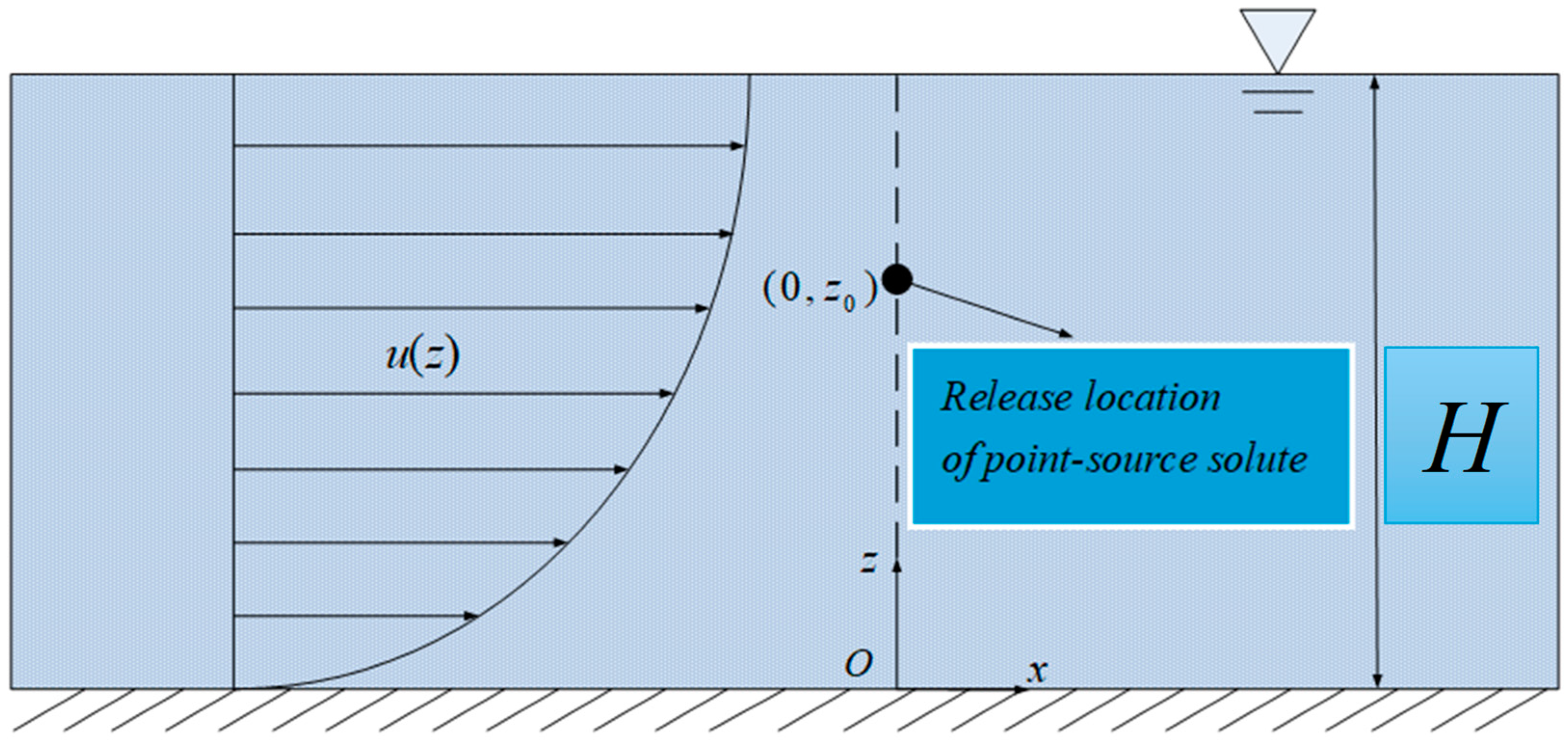
2.1. Review of the Case for Single-Point-Source Solute Instantaneous Release

A two-dimensional model for the point-source solute transport–diffusion process is depicted in Figure 1 below. It assumes an instantaneous release of solute at any vertical position within the flow channel [13,17,18].

Within the framework of the phase-average theory [12,13], the governing equation for an ideal two-dimensional model of a uniform material medium filled in a channel can be expressed as follows [13,17,18]:

$${\displaystyle \frac{\partial C}{\partial t}}+{\displaystyle \frac{u}{\varphi }}{\displaystyle \frac{\partial C}{\partial x}}=\kappa \left(\lambda +{\displaystyle \frac{K}{\varphi }}\right)\left({\displaystyle \frac{{\partial }^{2}C}{\partial x^2}}+{\displaystyle \frac{{\partial }^{2}C}{\partial z^2}}\right)$$

(1)

Considering the instantaneous release of a point-source solute with a mass of Q at an arbitrary position $\left(0,z_0\right)$ within a flow channel, the initial-boundary conditions can be expressed as follows according to references [13,17,18]:

$${C\left(x,z,t\right)|}_{t=0}=Q \delta \left(x\right) \delta \left(z-z_0\right)$$

(2)

$${C\left(x,z,t\right)|}_{x=\pm \infty }=0$$

(3)

$${{\displaystyle \frac{\partial C}{\partial z}}|}_{z=0}={{\displaystyle \frac{\partial C}{\partial z}}|}_{z=H}=0$$

(4)

Here, C indicates the spatial distribution of concentration; t denotes the time variable; x represents the flow coordinates; z represents the vertical coordinates; z₀ denotes the vertical position of the released solute; u is the flow velocity distribution function, which is only related to the vertical coordinate variable z; Φ represents the porosity of the flow channel; κ represents the tortuosity; λ represents the mass diffusion coefficient; K represents the mass dispersion; Q represents the mass of the released solute; and H represents the depth of the flow channel. δ(x) is the Dirac impulse function, proposed by the renowned physicist Dirac in the 1920s during his studies in quantum mechanics, which can physically describe the effects of instantaneous action (instantaneous force, impulse, matter source, etc.) and is mathematically defined in [19,20]:

$$\delta \left(x\right)=\{\begin{array}{ll}+\infty & x=0\\ 0& x\ne 0\end{array}$$

(5)

δ(x) satisfies the following integral relations [19,20]:

$${\displaystyle {\int }_{-\infty }^{+\infty }\delta \left(x\right)}dx=1$$

(6)

$${\displaystyle {\int }_{-\infty }^{+\infty }f\left(x\right)\delta \left(x-x_0\right)dx=f\left(x_0\right)}$$

(7)

According to dimensionless derivations [13,17,18]:

$$\psi ={\displaystyle \frac{u}{\langle u\rangle }},Pe={\displaystyle \frac{\langle u\rangle H}{\varphi \kappa \left(\lambda +\frac{K}{\varphi }\right)}},t^{*}={\displaystyle \frac{t\varphi \kappa \left(\lambda +\frac{K}{\varphi }\right)}{H^2}},\mathsf{\Omega }={\displaystyle \frac{C{H}^2}{Q}},\eta ={\displaystyle \frac{x}{H}}-Pe{t}^{*},\zeta ={\displaystyle \frac{z}{H}}$$

The dimensionless equation and its initial-boundary conditions are as follows [13,17,18]:

$$\{\begin{array}{l}{\displaystyle \frac{\partial \mathsf{\Omega }}{\partial t^{*}}}+Pe{\psi }^{\prime }{\displaystyle \frac{\partial \mathsf{\Omega }}{\partial \eta }}={\displaystyle \frac{{\partial }^2\mathsf{\Omega }}{\partial {\eta }^2}}+{\displaystyle \frac{{\partial }^2\mathsf{\Omega }}{\partial {\zeta }^2}}\\ \mathsf{\Omega }\left(\eta ,\zeta ,t^{*}\right){|}_{t^{*}=0}=\delta \left(\eta \right) \delta \left(\zeta -{\zeta }_0\right)\\ {{\displaystyle \frac{\partial \mathsf{\Omega }}{\partial \zeta }}|}_{\zeta =0}={{\displaystyle \frac{\partial \mathsf{\Omega }}{\partial \zeta }}|}_{\zeta =1}=0\\ {\mathsf{\Omega }\left(\eta ,\zeta ,t^{*}\right)|}_{\eta =\pm \infty }=0\end{array}$$

(8)

In the above formula, Ω represents the dimensionless concentration, t^* is the dimensionless time, Pe is the Peclet number, which physically directly reflects the magnitude of the fluid convection intensity, η is the dimensionless streamwise coordinate, ζ is the dimensionless vertical coordinate (ζ is between 0 and 1), and ζ₀ is the dimensionless solute vertical release point (ζ₀ is between 0 and 1). The dimensionless velocity deviation, as defined in references [13,17,18], is as follows:

$${\psi }^{\prime }=\psi -\langle \psi \rangle$$

(9)

In a two-dimensional flow, the cross-sectional average operator $\langle \cdot \rangle$ is the vertical average or spanwise average operator. It is mathematically defined in references [13,17,18]:

$$\langle \cdot \rangle ={\displaystyle {\int }_0^1\cdot d\zeta }$$

(10)

As mentioned above, to avoid the difficulty of a direct analytical solution, Equation (8) can be mathematically handled using the Aris concentration moment method. For the two-dimensional flow model discussed in this paper, as defined in references [13,17,18], the p-order concentration moment, concentration moment operator, and assumptions of the concentration distribution attenuation conditions that adhere to physical facts are, respectively, as follows:

$$m_p\left(\zeta ,t^{*}\right)={\displaystyle {\int }_{-\infty }^{\infty }\mathsf{\Omega }\left(\eta ,\zeta ,t^{*}\right)} {\eta }^p \mathrm{d}\eta , (p=0, 1, 2\dots )$$

(11)

$${\displaystyle {\int }_{-\infty }^{\infty }\cdot } {\eta }^p \mathrm{d}\eta , (p=0, 1, 2\dots )$$

(12)

$$\begin{array}{l}\eta \mathsf{\Omega }{|}_{\eta =\pm \infty }={\eta }^2\mathsf{\Omega }{|}_{\eta =\pm \infty }=\dots ={\eta }^p\mathsf{\Omega }{|}_{\eta =\pm \infty }=0,\\ {\displaystyle \frac{\partial \mathsf{\Omega }}{\partial \eta }}{|}_{\eta =\pm \infty }=\eta {\displaystyle \frac{\partial \mathsf{\Omega }}{\partial \eta }}{|}_{\eta =\pm \infty }={\eta }^2{\displaystyle \frac{\partial \mathsf{\Omega }}{\partial \eta }}{|}_{\eta =\pm \infty }=\dots ={\eta }^p{\displaystyle \frac{\partial \mathsf{\Omega }}{\partial \eta }}{|}_{\eta =\pm \infty }=0\end{array}$$

(13)

The p-order concentration moment operator index p is taken as 0 and 1, representing the zeroth-order and first-order concentration moment operators. These two operators are applied to Equation (8) while considering the concentration distribution attenuation conditions. Subsequently, the zeroth-order and first-order concentration moment equations, along with the initial-boundary conditions, can be derived [8,17,18]. Specifically, the zeroth-order concentration moment and first-order concentration moment satisfy the following equations and conditions [8,17,18]:

$$\{\begin{array}{l}{\displaystyle \frac{\partial m_0}{\partial t^{*}}}={\displaystyle \frac{{\partial }^2{m}_0}{\partial {\zeta }^2}}\\ {{\displaystyle \frac{\partial m_0}{\partial \zeta }}|}_{\zeta =0}={{\displaystyle \frac{\partial m_0}{\partial \zeta }}|}_{\zeta =1}=0\\ m_0\left(\zeta ,t^{*}\right){|}_{t^{*}=0}=\delta \left(\zeta -{\zeta }_0\right)\end{array}$$

(14)

$$\{\begin{array}{l}{\displaystyle \frac{\partial m_1}{\partial t^{*}}}={\displaystyle \frac{{\partial }^2{m}_1}{\partial {\zeta }^2}}+Pe{\psi }^{\prime }{m}_0\\ {{\displaystyle \frac{\partial m_1}{\partial \zeta }}|}_{\zeta =0}={{\displaystyle \frac{\partial m_1}{\partial \zeta }}|}_{\zeta =1}=0\\ {m_1\left(\zeta ,t^{*}\right)|}_{t^{*}=0}=0\end{array}$$

(15)

Theoretically, if the zeroth-order and first-order concentration moment equations can be solved successfully, that is, analytical expressions for them can be obtained, it is of great significance for analyzing the conservation of solute mass, analyzing the movement of the centroid of mass, and predicting the solute concentration distribution [8,17,18].

From a physical perspective, if one wants to master the information of the total mass of solute released at any time in the transport and dispersion process, one only needs to perform a cross-sectional average operation on the zeroth-order concentration moment, namely [8,17,18]:

$$\langle m_0\rangle ={\displaystyle {\int }_0^1{m}_0\left(\zeta ,t^{*}\right)}d\zeta$$

(16)

To investigate the displacement of the centroid movement of the released solute at any time during the transport–dispersion process, one only needs to perform a cross-sectional average operation on the first-order concentration moment and then divide it by the cross-sectional average, namely [8,17,18]:

$$\mathsf{\Delta }\eta ={\displaystyle \frac{\langle m_1\rangle }{\langle m_0\rangle }}={\displaystyle \frac{{\displaystyle {\int }_0^1{\displaystyle {\int }_{-\infty }^{+\infty }\mathsf{\Omega }\eta d\eta d\zeta }}}{{\displaystyle {\int }_0^1{\displaystyle {\int }_{-\infty }^{+\infty }\mathsf{\Omega }d\eta d\zeta }}}}$$

(17)

Following the classical Taylor dispersion theory, if we observe a moving coordinate system that moves with the average velocity, the cross-sectional average concentration satisfies the following equation [8,13,17,18]:

$${\displaystyle \frac{\partial \langle \mathsf{\Omega }\rangle }{\partial t^{*}}}=D{\displaystyle \frac{{\partial }^2\langle \mathsf{\Omega }\rangle }{\partial {\eta }^2}}$$

(18)

Here, D represents the Taylor dispersion coefficient. After a long period of evolution, in the case of a solute released from a line source (with a uniform distribution of solute at the initial moment), the cross-sectional mean concentration of the solute (that is, $\langle {\mathsf{\Omega }}_0\rangle$) shows a classical Gaussian distribution. If the long-term asymptotic value of the dispersion coefficient is denoted as $D_T$, $\langle {\mathsf{\Omega }}_0\rangle$ can be expressed as [8,13,17,18]:

$$\langle {\mathsf{\Omega }}_0\rangle ={\displaystyle \frac{1}{\sqrt{4\pi D_T{t}^{*}}}}{e}^{-{\displaystyle \frac{{\eta }^2}{4D_T{t}^{*}}}}$$

(19)

In the case of point-source release, based on the line-source solution obtained (19), after a long period of evolution, the expression for the average concentration of solute released from a point source (that is, $\langle \mathsf{\Omega }\rangle$) can be obtained as follows [8,17,18]:

$$\langle \mathsf{\Omega }\rangle ={\displaystyle \frac{1}{\sqrt{4\pi D_T{t}^{*}}}}{e}^{-{\displaystyle \frac{{\left(\eta -\mathsf{\Delta }\eta \right)}^2}{4D_T{t}^{*}}}}$$

(20)

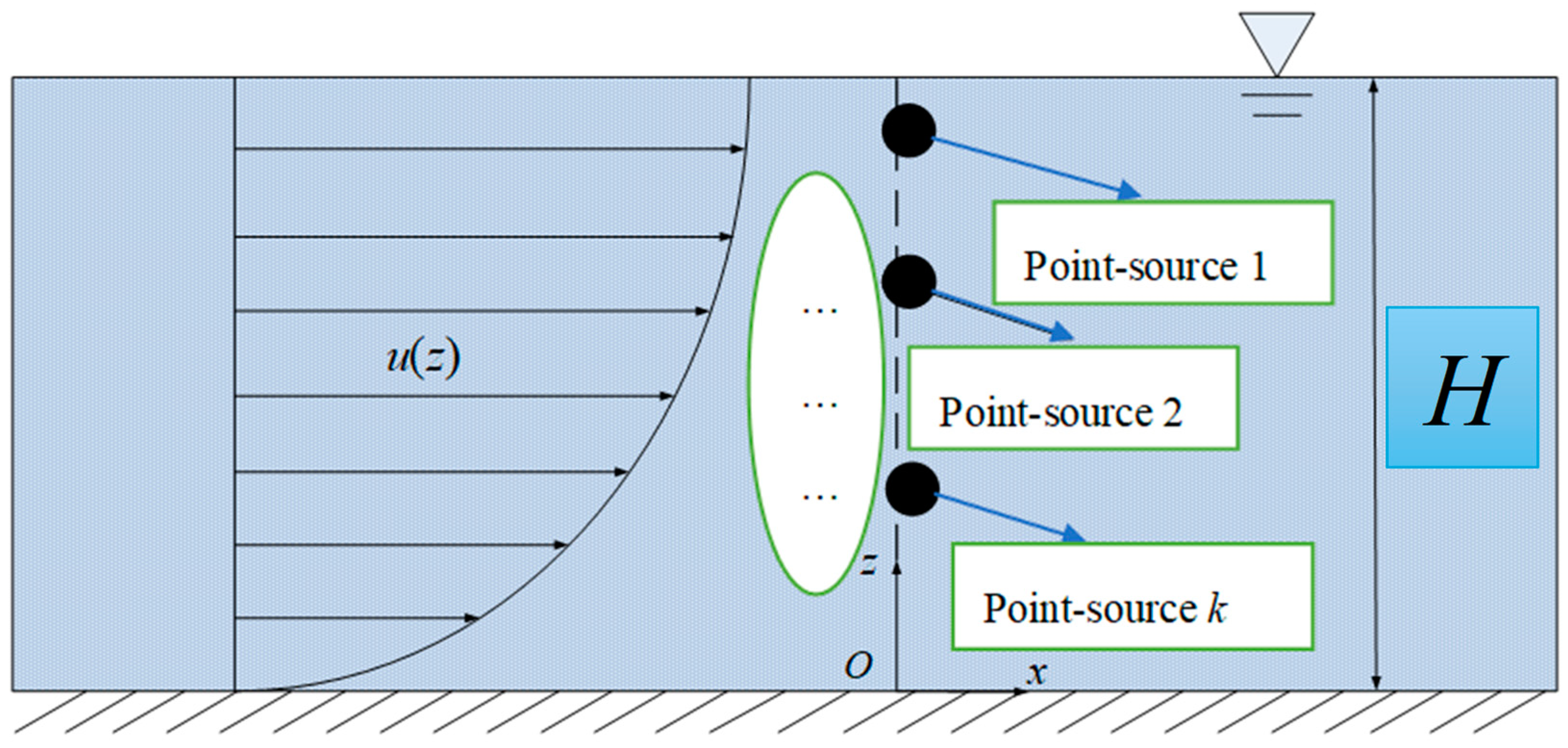
2.2. Generalization of Instantaneous Release of Multi-Point-Source Solute

In particular, due to the requirements of theoretical research and engineering applications, it is essential to extend the single-point-source release model to a multi-point-source release model. This applies to scenarios like multi-point-source industrial wastewater, multi-point-source municipal sewage, and multi-point-source pollution transported to water bodies through urban sewage treatment plants or pipe canals. This extension implies that there are multiple discharge outlets simultaneously releasing pollutants. The vertical coordinate of the k-th discharge outlet is z_k, with an instantaneous emission of Q_k. The total emission from all k discharge outlets is Q.

Figure 2 is the model of multi-point-source solute instantaneous release (schematic). The transport–diffusion equation and the initial-boundary conditions of the multi-point-source solute instantaneous release model can be written as follows:

$$\{\begin{array}{l}{\displaystyle \frac{\partial C}{\partial t}}+{\displaystyle \frac{u}{\varphi }}{\displaystyle \frac{\partial C}{\partial x}}=\kappa \left(\lambda +{\displaystyle \frac{K}{\varphi }}\right)\left({\displaystyle \frac{{\partial }^{2}C}{\partial x^2}}+{\displaystyle \frac{{\partial }^{2}C}{\partial z^2}}\right)\\ {C\left(x,z,t\right)|}_{t=0}={\displaystyle \sum _{l=1}^k{Q}_l \delta \left(x\right) \delta \left(z-z_l\right)}\\ {C\left(x,z,t\right)|}_{x=\pm \infty }=0\\ {{\displaystyle \frac{\partial C}{\partial z}}|}_{z=0}={{\displaystyle \frac{\partial C}{\partial z}}|}_{z=H}=0\\ {\displaystyle \sum _{l=1}^k{Q}_l}=Q \end{array}$$

(21)

If $C_l$ and ${\mathsf{\Omega }}_l$ satisfy the concentration equation (in dimensional form) and the corresponding dimensionless concentration equation (where l = 1,2, …, k), the following equations, respectively, can be obtained:

$$\{\begin{array}{l}{\displaystyle \frac{\partial C_l}{\partial t}}+{\displaystyle \frac{u}{\varphi }}{\displaystyle \frac{\partial C_l}{\partial x}}=\kappa \left(\lambda +{\displaystyle \frac{K}{\varphi }}\right)\left({\displaystyle \frac{{\partial }^2{C}_l}{\partial x^2}}+{\displaystyle \frac{{\partial }^2{C}_l}{\partial z^2}}\right)\\ {C_l\left(x,z,t\right)|}_{t=0}=Q_l \delta \left(x\right) \delta \left(z-z_l\right)\\ {C_l\left(x,z,t\right)|}_{x=\pm \infty }=0\\ {{\displaystyle \frac{\partial C_l}{\partial z}}|}_{z=0}={{\displaystyle \frac{\partial C_l}{\partial z}}|}_{z=H}=0\end{array}$$

(22)

$$\{\begin{array}{l}{\displaystyle \frac{\partial {\mathsf{\Omega }}_l}{\partial t^{*}}}+Pe{\psi }^{\prime }{\displaystyle \frac{\partial {\mathsf{\Omega }}_l}{\partial \eta }}={\displaystyle \frac{{\partial }^2{\mathsf{\Omega }}_l}{\partial {\eta }^2}}+{\displaystyle \frac{{\partial }^2{\mathsf{\Omega }}_l}{\partial {\zeta }^2}}\\ {{\mathsf{\Omega }}_l\left(\eta ,\zeta ,t^{*}\right)|}_{\tau =0}=\delta \left(\eta \right) \delta \left(\zeta -{\zeta }_l\right)\\ {{\mathsf{\Omega }}_l\left(\eta ,\zeta ,t^{*}\right)|}_{\eta =\pm \infty }=0\\ {{\displaystyle \frac{\partial {\mathsf{\Omega }}_l}{\partial \zeta }}|}_{\zeta =0}={{\displaystyle \frac{\partial {\mathsf{\Omega }}_l}{\partial \zeta }}|}_{\zeta =1}=0\end{array}$$

(23)

Thus, according to the superposition principle of linear equation solutions, the solution C of Equation (21) is expressed as follows:

$$C={\displaystyle \sum _{l=1}^k{C}_l}$$

(24)

We assume that the instantaneous release of solutes at each discharge outlet has the same chemical composition (no chemical reactions occur).

Incidentally, for a water environmental flow with an approximately linear velocity distribution (for which $u\left(z\right)$ can be treated as a linear function of the vertical coordinate z, similar to the ideal physical model of Couette flow), considering k discharge outlets simultaneously discharging, resorting to the concept of mass centroid, it is physically equivalent to the instantaneous release of solute mass Q at the centroid position of these point-source solutes. The centroid position can be easily calculated as:

$$z_c={\displaystyle \frac{Q_1{z}_1+Q_2{z}_2+\cdots Q_k{z}_k}{Q_1+Q_2+\cdots Q_k}}={\displaystyle \frac{Q_1{z}_1+Q_2{z}_2+\cdots Q_k{z}_k}{Q}}$$

(25)

Therefore, the equation that can approximately describe the transport–diffusion process of a multi-point-source solute instantaneous release can be given as follows:

$$\{\begin{array}{l}{\displaystyle \frac{\partial C}{\partial t}}+{\displaystyle \frac{u}{\varphi }}{\displaystyle \frac{\partial C}{\partial x}}=\kappa \left(\lambda +{\displaystyle \frac{K}{\varphi }}\right)\left({\displaystyle \frac{{\partial }^{2}C}{\partial x^2}}+{\displaystyle \frac{{\partial }^{2}C}{\partial z^2}}\right)\\ {C\left(x,z,t\right)|}_{t=0}=Q \delta \left(x\right) \delta \left(z-z_c\right)\\ {C\left(x,z,t\right)|}_{x=\pm \infty }=0\\ {{\displaystyle \frac{\partial C}{\partial z}}|}_{z=0}={{\displaystyle \frac{\partial C}{\partial z}}|}_{z=H}=0\end{array},z_c={\displaystyle \frac{Q_1{z}_1+Q_2{z}_2+\cdots Q_k{z}_k}{Q}}$$

(26)

It is evident that applying the separation of variables method to analyze the concentration moment equation of a single-point-source release allows for a convenient solution to the case of multi-point-source releases.

3. Solving the Solute Concentration Moment Equation Using the Separation of Variables Method

3.1. Zeroth-Order Concentration Moment Solution

From the previous descriptions, it is clear that the analytical solutions of the zeroth-order moment $m_0\left(\zeta ,t^{*}\right)$ and first-order moment $m_1\left(\zeta ,t^{*}\right)$ are of great value for theoretical research. Previous studies applied the integral transformation method to solve the equations with corresponding initial-boundary value conditions [17,18]. In the following section, the two equations above will be solved using the classical separation of variables method, which has been widely employed in solving eigenvalue problems in linear mathematical physics. Through the separation of variables method, the exact analytical solutions will be derived (suitable for physical flow velocity distribution), which is convenient for further theoretical discussions.

For the zeroth-order moment equation and its initial-boundary value conditions (14), suppose that $m_0={\varphi }_1\left(t^{*}\right){\varphi }_2\left(\zeta \right),$ and substituting into the zeroth-order moment equation, we have:

$${{\varphi }_1}^{\prime }\left(t^{*}\right){\varphi }_2\left(\zeta \right)={\varphi }_1\left(t^{*}\right){{\varphi }_2}^{″}\left(\zeta \right)$$

(27)

Rewriting it, we obtain:

$${\displaystyle \frac{{{\varphi }_1}^{\prime }\left(t^{*}\right)}{{\varphi }_1\left(t^{*}\right)}}={\displaystyle \frac{{{\varphi }_2}^{″}\left(\zeta \right)}{{\varphi }_2\left(\zeta \right)}}=\lambda$$

(28)

The values of λ are discussed in the following three cases.

<i> λ = 0

We have ${\varphi }_1^{\prime }\left(t^{*}\right)=0,{{\varphi }_2}^{″}\left(\zeta \right)=0$, and then:

$$\begin{array}{l}{\varphi }_1\left(t^{*}\right)=c_1,\\ {\varphi }_2\left(\zeta \right)=c_2\zeta +c_3\end{array}$$

(29)

Considering the boundary condition, we have c₂ = 0, and c₁ and c₃ are both non-zero (otherwise it would lead to a zero solution). Therefore, for λ = 0, we obtain a constant function (non-zero), which will be utilized in <iii> (for λ < 0).

<ii> λ > 0

We have ${\varphi }_2\left(\zeta \right)=c_1{e}^{\sqrt{\lambda }\zeta }+c_2{e}^{-\sqrt{\lambda }\zeta }$, and when considering the initial boundary conditions, it becomes evident that $c_1=c_2=0$, which leads to a zero solution. Therefore, <ii> can be ruled out.

<iii> λ < 0

For ${\varphi }_2$, we have:

$$\begin{array}{l}{{\varphi }_2}^{″}\left(\zeta \right)-\lambda {\varphi }_2\left(\zeta \right)=0\\ {{{\varphi }_2}^{\prime }\left(\zeta \right)|}_{\zeta =0}={{{\varphi }_2}^{\prime }\left(\zeta \right)|}_{\zeta =1}=0\end{array}$$

(30)

Solving the ordinary differential equation and its boundary conditions above, we have:

$${\varphi }_2\left(\zeta \right)=A\cdot \cos \left(\sqrt{-\lambda }\cdot \zeta \right)+B\cdot \sin \left(\sqrt{-\lambda }\cdot \zeta \right)$$

Using the boundary conditions, we can obtain B = 0, then,

$${\varphi }_2\left(\zeta \right)=A\cdot \cos \left(\sqrt{-\lambda }\cdot \zeta \right)$$

and

$$\lambda =-{\left(n\pi \right)}^2,n=1,2,3,\dots$$

Thus, for ${\varphi }_2$,

$$\begin{array}{l}{\varphi }_2\left(\zeta \right)=A_n\cdot \cos \left(n\pi \zeta \right)\\ n=1,2,3,\dots \end{array}$$

(31)

and for ${\varphi }_1$, we have:

$${{\varphi }_1}^{\prime }\left(t^{*}\right)-\lambda {\varphi }_1\left(t^{*}\right)=0$$

(32)

Solving it, we obtain:

$${\varphi }_1\left(t^{*}\right)=C\cdot e^{-\lambda t^{*}}=C_n\cdot e^{-n^2{\pi }^2{t}^{*}}$$

(33)

Thus, we obtain a family of functions:

$$\left\{c_n\cdot \cos \left(n\pi \zeta \right)\cdot e^{-n^2{\pi }^2{t}^{*}}\right\},n=1,2,3,\cdots$$

Here, $c_n=A_n\cdot C_n$

According to the value of the indicator n, as well as the case <i> (that is, λ = 0, which means n = 0), we can create a linear superposition. The analytical expression of $m_0$ is given as follows:

$$m_0\left(\zeta ,t^{*}\right)=c_0+{\displaystyle \sum _{n=1}^{\infty }{c}_n\cos \left(n\pi \zeta \right)\cdot e^{-n^2{\pi }^2{t}^{*}}}$$

(34)

In order to determine the value of coefficients $c_n$, we resort to the orthogonality of the trigonometric function family. This means that:

$${\displaystyle {\int }_0^1\cos \left(n\pi \zeta \right)\cdot \cos \left(m\pi \zeta \right)}d\zeta =\{\begin{array}{cc}0,& n\ne m\\ {\displaystyle \frac{1}{2}},& n=m\end{array}$$

(35)

The two sides of the equation are multiplied by cos(nπζ) and then integrated:

$${\displaystyle {\int }_0^1{c}_n\cos \left(n\pi \zeta \right)\cdot \cos \left(n\pi \zeta \right)}d\zeta ={\displaystyle \frac{1}{2}}{c}_n={\displaystyle {\int }_0^1\delta \left(\zeta -{\zeta }_0\right)}\cos \left(n\pi \zeta \right)d\zeta$$

(36)

Using the property of the Dirac delta function, we obtain:

$${\displaystyle {\int }_0^1\delta \left(\zeta -{\zeta }_0\right)}\cos \left(n\pi \zeta \right)d\zeta =\cos \left(n\pi {\zeta }_0\right)$$

(37)

Thus, we have:

$$c_n=2\cos \left(n\pi {\zeta }_0\right),n=1,2,3,\cdots$$

(38)

Here, $c_0={\displaystyle {\int }_0^1\delta \left(\zeta -{\zeta }_0\right)}d\zeta =1$, and ${\zeta }_0$ represents the dimensionless vertical position of the released solute, so we have:

$$m_0\left(\zeta ,t^{*}\right)=1+2{\displaystyle \sum _{n=1}^{\infty }\cos \left(n\pi {\zeta }_0\right)\cos \left(n\pi \zeta \right)\cdot e^{-n^2{\pi }^2{t}^{*}}}$$

(39)

The result obtained above using the separation of variables method is consistent with the solution obtained through an integral transform in a previous study [17,18]. This also demonstrates the effectiveness of the separation of variables method.

For the zero-order concentration moment, the cross-sectional average operation is performed:

$$\langle m_0\rangle ={\displaystyle {\int }_0^1\left\{1+2{\displaystyle \sum _{n=1}^{\infty }\cos \left(n\pi {\zeta }_0\right)\cos \left(n\pi \zeta \right)\cdot e^{-n^2{\pi }^2{t}^{*}}}\right\}}d\zeta$$

(40)

According to the uniform convergence property of function term series (39), we can perform term-by-term integration:

$$\langle m_0\rangle ={\displaystyle {\int }_0^{1}1d\zeta }+2{\displaystyle \sum _{n=1}^{\infty }\left\{{\displaystyle {\int }_0^1\cos \left(n\pi {\zeta }_0\right)\cos \left(n\pi \zeta \right)\cdot e^{-n^2{\pi }^2{t}^{*}}d}\zeta \right\}}=1$$

(41)

Mathematically, dηdζ can be treated as the “volume of a differential element”. Ω represents the concentration (can be treated as density), and Ωdηdζ represents the “mass of a differential element”. Because the integral ranges of η and ζ are from 0 to 1 and $-\infty$ to $+\infty$, respectively, the integral (40) traverses the entire flow channel space. $\langle m_0\rangle$ represents the mass of the whole released solute, and $\langle m_0\rangle =1$ illustrates the conservation of solute mass during the entire transport–diffusion–dispersion process. This interpretation is also consistent with conclusions in previous literature [8,17].

3.2. First-Order Concentration Moment Solution

Different from the zeroth-order concentration moment Equation (14), the first-order concentration moment Equation (15) is a non-homogeneous equation. Therefore, Equation (15) needs to be homogenized using relevant mathematical techniques before applying the separation of variables method to solve it. Subsequently, an important theorem known as Duhamel’s homogenization principle [19] can be introduced, followed by a concise mathematical proof.

Theorem 1 (Duhamel’s Principle).

For a non-homogeneous equation with its initial-boundary condition:

$$\{\begin{array}{l}{u}_t=a^2{u}_{xx}+f\left(x,t\right)\\ {u_x|}_{x=0}={u_x|}_{x=l}=0\\ {u|}_{t=0}=0\end{array}$$

(42)

Consider the solution $w(x,t;\tau )$ of:

$$\{\begin{array}{l}{w}_t=a^2{w}_{xx}\hspace{1em}\hspace{1em}t>\tau \\ {w_x|}_{x=0}={w_x|}_{x=l}=0\\ {w|}_{t=\tau }=f\left(x;\tau \right)\end{array}$$

(43)

Then, perform the integral operation:

$$u\left(x,t\right)={\displaystyle {\int }_0^{t}w\left(x,t;\tau \right)d\tau }$$

(44)

Thus, $u(x,t)$ is the exact solution of (42).

Proof. 

Considering $u\left(x,t\right)={\displaystyle {\int }_0^{t}w\left(x,t;\tau \right)d\tau }$, calculate partial derivatives:

$$\begin{array}{l}{u}_t\left(x,t\right)={\displaystyle {\int }_0^t{w}_t\left(x,t;\tau \right)d\tau }+f\left(x,t\right)\\ u_x={\displaystyle {\int }_0^t{w}_x\left(x,t;\tau \right)d\tau },u_{xx}={\int }_0^t{w}_{xx}\left(x,t;\tau \right)d\tau \end{array}$$

(45)

Here, $w_t=a^2{w}_{xx}$, the integral operation is ${\displaystyle {\int }_0^t{w}_{t}d\tau =}{a}^2{\displaystyle {\int }_0^t{w}_{xx}d\tau }$, and then:

$${\displaystyle {\int }_0^t{w}_{t}d\tau }+f\left(x,t\right)=a^2{\displaystyle {\int }_0^t{w}_{xx}d\tau }+f\left(x,t\right)$$

(46)

That is,

$$u_t=a^2{u}_{xx}+f\left(x,t\right)$$

(47)

If t = 0,

$$u\left(x,0\right)={\displaystyle {\int }_0^{0}w\left(x,t;\tau \right)d\tau }=0$$

(48)

then:

$${u|}_{t=0}=0$$

(49)

When x = 0 and x = l,

$$\begin{array}{l}{u_x|}_{x=0}={\displaystyle {\int }_0^t{w_x|}_{x=0}d\tau }=0,\\ {u_x|}_{x=l}={\displaystyle {\int }_0^t{w_x|}_{x=l}d\tau }=0\end{array}$$

(50)

It shows that u(x,t) is the solution of the original, non-homogeneous Equation (42). □

From the above theorem, to realize the solution of Equation (15), we need to consider the following homogeneous problem:

$$\{\begin{array}{l}{w}_{t^{*}}=w_{\zeta \zeta },\hspace{1em}{t}^{*}>\tau \\ {w_{\zeta }|}_{\zeta =0}={w_{\zeta }|}_{\zeta =1}=0\\ {w|}_{t^{*}=\tau }=Pe{\psi }^{\prime }{m}_0\end{array}$$

(51)

If we can find the solution $w\left(\zeta ,t^{*};\tau \right)$ of Equation (51), then the first-order concentration moment $m_1\left(\zeta ,t^{*}\right)={\displaystyle {\int }_0^{t^{*}}w\left(\zeta ,t^{*};\tau \right)}d\tau$ can be obtained.

Applying the separation of variables method to Equation (51), suppose the following:

$$w\left(\zeta ,t^{*};\tau \right)={\varphi }_1\left(\zeta ;\tau \right){\varphi }_2\left(t^{*};\tau \right)$$

(52)

Thus,

$$\begin{array}{l}{w}_{t^{*}}={\varphi }_1\left(\zeta ;\tau \right){\displaystyle \frac{d{\varphi }_2\left(t^{*};\tau \right)}{d{t}^{*}}},\\ w_{\zeta \zeta }={\varphi }_2\left(t^{*};\tau \right){\displaystyle \frac{d^2{\varphi }_1\left(\zeta ;\tau \right)}{d{\zeta }^2}}\end{array}$$

(53)

Substituting above formulas into the equation yields:

$${\displaystyle \frac{{{\varphi }_1}^{″}\left(\zeta ;\tau \right)}{{\varphi }_1\left(\zeta ;\tau \right)}}={\displaystyle \frac{{{\varphi }_2}^{\prime }\left(t^{*};\tau \right)}{{\varphi }_2\left(t^{*};\tau \right)}}=g\left(\tau \right)$$

(54)

Similar to the solution procedures in Equation (14), the values of $g\left(\tau \right)$ can be discussed in the following three cases:

<i> $g\left(\tau \right)=0$

Then, ${{\varphi }_1}^{″}\left(\zeta ;\tau \right)={{\varphi }_2}^{\prime }\left(t^{*};\tau \right)=0$, so we obtain:

$$\begin{array}{l}{\varphi }_1\left(\zeta ;\tau \right)=g_1\left(\tau \right)\zeta +g_2\left(\tau \right),\\ {\varphi }_2\left(t^{*};\tau \right)=g_3\left(\tau \right)\end{array}$$

(55)

That is, $w\left(\zeta ,t^{*};\tau \right)=\left[g_1\left(\tau \right)g_3\left(\tau \right)\right]\zeta +g_2\left(\tau \right)g_3\left(\tau \right)$.

Due to the boundary conditions of ${\left.w_{\zeta }\right|}_{\zeta =0}={\left.w_{\zeta }\right|}_{\zeta =1}=0$, $g_1\left(\tau \right)\cdot g_3\left(\tau \right)=0$.

If $g_3\left(\tau \right)=0$, then $w\left(\zeta ,t^{*};\tau \right)=0$, which leads to a zero solution, so the case of $g_3\left(\tau \right)=0$ can be ruled out; so, $g_1(\tau )=0$, then, $w\left(\zeta ,t^{*};\tau \right)=c_0\left(\tau \right)$ (here, $c_0\left(\tau \right)=g_2\left(\tau \right)g_3\left(\tau \right),g_2\left(\tau \right)\ne 0,g_3\left(\tau \right)\ne 0$; otherwise, it leads to a zero solution). Thus, for $g(\tau )=0$, we obtain a function related only to $\tau$ (that is, $c_0\left(\tau \right)$, non-zero solution). It will be utilized in <iii> (for $g\left(\tau \right)<0$).

<ii> $g\left(\tau \right)>0$

That is, ${{\varphi }_1}^{″}\left(\zeta ;\tau \right)-g\left(\tau \right){\varphi }_1\left(\zeta ;\tau \right)=0$, and ${{\varphi }_2}^{\prime }\left(t^{*};\tau \right)-g\left(\tau \right){\varphi }_2\left(t^{*};\tau \right)=0$; ${\varphi }_1,{\varphi }_2$ can both be solved:

$$\begin{array}{l}{\varphi }_1\left(\zeta ;\tau \right)=c_1\left(\tau \right)e^{\sqrt{g\left(\tau \right)}.\zeta }+c_2\left(\tau \right)e^{-\sqrt{g\left(\tau \right)}.\zeta },\\ {\varphi }_2\left(t^{*};\tau \right)=c_3\left(\tau \right)e^{g\left(\tau \right).t^{*}}\end{array}$$

(56)

Then:

$$\begin{array}{l}w\left(\zeta ,t^{*};\tau \right)=c_1\left(\tau \right)c_3\left(\tau \right)e^{\sqrt{g\left(\tau \right)}.\zeta +g\left(\tau \right).t^{*}}+c_2\left(\tau \right)c_3\left(\tau \right)e^{-\sqrt{g\left(\tau \right)}.\zeta +g\left(\tau \right).t^{*}},\\ w_{\zeta }=c_1\left(\tau \right)c_3\left(\tau \right)\sqrt{g\left(\tau \right)}{e}^{\sqrt{g\left(\tau \right)}.\zeta +g\left(\tau \right).t^{*}}-c_2\left(\tau \right)c_3\left(\tau \right)\sqrt{g\left(\tau \right)}{e}^{-\sqrt{g\left(\tau \right)}.\zeta +g\left(\tau \right).t^{*}}\end{array}$$

(57)

According to boundary conditions, we can obtain the following:

$$\begin{array}{l}{c}_1\left(\tau \right)c_3\left(\tau \right)\sqrt{g\left(\tau \right)}{e}^{g\left(\tau \right).t^{*}}-c_2\left(\tau \right)c_3\left(\tau \right)\sqrt{g\left(\tau \right)}{e}^{g\left(\tau \right).t^{*}}=0,\\ c_1\left(\tau \right)c_3\left(\tau \right)\sqrt{g\left(\tau \right)}{e}^{\sqrt{g\left(\tau \right)}+g\left(\tau \right).t^{*}}-c_2\left(\tau \right)c_3\left(\tau \right)\sqrt{g\left(\tau \right)}{e}^{-\sqrt{g\left(\tau \right)}+g\left(\tau \right).t^{*}}=0\end{array}$$

(58)

Here $g\left(\tau \right)>0,c_3\left(\tau \right)\ne 0$, and then:

$$\{\begin{array}{l}{c}_1\left(\tau \right)-c_2\left(\tau \right)=0\\ c_1\left(\tau \right)e^{\sqrt{g\left(\tau \right)}}-c_2\left(\tau \right)e^{-\sqrt{g\left(\tau \right)}}=0\end{array}$$

(59)

Because the coefficient determinant $\left|\begin{array}{cc}1& -1\\ e^{\sqrt{g\left(\tau \right)}}& -e^{-\sqrt{g\left(\tau \right)}}\end{array}\right|\ne 0$, we can resort to Kramer’s rule of linear algebra, and Equation (59) only has a zero solution, which means that $c_1\left(\tau \right)=c_2\left(\tau \right)=0$, ${\varphi }_1\left(\zeta ;\tau \right)=0$; this leads to a zero solution, so <ii> can be ruled out.

<iii> $g\left(\tau \right)<0$

That is,

$$\begin{array}{l}{{\varphi }^{″}}_1\left(\zeta ;\tau \right)-g\left(\tau \right){\varphi }_1\left(\zeta ;\tau \right)=0,\\ {{\varphi }^{\prime }}_2\left(t^{*};\tau \right)-g\left(\tau \right){\varphi }_2\left(t^{*};\tau \right)=0\end{array}$$

(60)

${\varphi }_1,{\varphi }_2$ can be solved as follows:

$$\begin{array}{l}{\varphi }_1\left(\zeta ;\tau \right)=c_1\left(\tau \right)\cos \left(\sqrt{-g\left(\tau \right)}\cdot \zeta \right)+c_2\left(\tau \right)\sin \left(\sqrt{-g\left(\tau \right)}\cdot \zeta \right),\\ {\varphi }_2\left(t^{*};\tau \right)=c_3\left(\tau \right)e^{g\left(\tau \right).t^{*}}\end{array}$$

(61)

Thus,

$$\begin{array}{l}w=c_3\left(\tau \right)e^{g\left(\tau \right).t^{*}}\\ \cdot \left[c_1\left(\tau \right)\cos \left(\sqrt{-g\left(\tau \right)}\cdot \zeta \right)+c_2\left(\tau \right)\sin \left(\sqrt{-g\left(\tau \right)}\cdot \zeta \right)\right],\\ w_{\zeta }=c_3\left(\tau \right)e^{g\left(\tau \right).t^{*}}\sqrt{-g\left(\tau \right)}\\ \cdot \left[c_2\left(\tau \right)\cos \left(\sqrt{-g\left(\tau \right)}\cdot \zeta \right)-c_1\left(\tau \right)\sin \left(\sqrt{-g\left(\tau \right)}\cdot \zeta \right)\right]\end{array}$$

(62)

Let $\zeta =0$, then:

$${w_{\zeta }|}_{\zeta =0}=c_3\left(\tau \right)e^{g\left(\tau \right).t^{*}}\cdot \sqrt{-g\left(\tau \right)}\cdot c_2\left(\tau \right)=0$$

(63)

$c_3\left(\tau \right)\ne 0$, $e^{g\left(\tau \right).t^{*}}>0$, and $\sqrt{-g\left(\tau \right)}>0$; thus, $c_2\left(\tau \right)=0$, so we obtain the following:

$$\begin{array}{l}w\left(\zeta ,t^{*};\tau \right)=c_3\left(\tau \right)e^{g\left(\tau \right).t^{*}}\cdot c_1(\tau )\cos \left(\sqrt{-g(\tau )}\cdot \zeta \right),\\ w_{\zeta }=c_3\left(\tau \right)e^{g\left(\tau \right).t^{*}}\cdot \sqrt{-g\left(\tau \right)}\cdot \left[-c_1(\tau )\sin (\sqrt{-g\left(\tau \right)}\cdot \zeta )\right],\\ {w_{\zeta }|}_{\zeta =1}=-c_1\left(\tau \right)c_3\left(\tau \right)\cdot \sqrt{-g\left(\tau \right)}\cdot e^{g\left(\tau \right).t^{*}}\cdot \sin \left(\sqrt{-g\left(\tau \right)}\right)=0\end{array}$$

(64)

Here, $c_3\left(\tau \right)\ne 0$, $\sqrt{-g\left(\tau \right)}>0$, $e^{g(\tau ).t^{*}}>0$, and $c_1\left(\tau \right)\ne 0$; thus, $\sin \left(\sqrt{-g\left(\tau \right)}\right)=0$. Then,

$$g\left(\tau \right)=-n^2{\pi }^2,n=1,2,3,\cdots$$

(65)

That is,

$$\begin{array}{l}w\left(\zeta ,t^{*};\tau \right)=c_3\left(\tau \right)e^{-n^2{\pi }^2{t}^{*}}\cdot c_1\left(\tau \right)\cos \left(n\pi \zeta \right),\\ n=1,2,3,\cdots \end{array}$$

(66)

Let $c\left(\tau \right)=c_1\left(\tau \right)c_3\left(\tau \right)$, then:

$$\begin{array}{l}w\left(\zeta ,t^{*};\tau \right)=c\left(\tau \right)e^{-n^2{\pi }^2{t}^{*}}\cdot \cos \left(n\pi \zeta \right),\\ n=1,2,3,\cdots \end{array}$$

(67)

Considering the case <i> (that is, $g(\tau )=0$; it means n = 0), similar to Equation (34), we can create a linear superposition:

$$\begin{array}{ll}w\left(\zeta ,t^{*};\tau \right)& =c_0\left(\tau \right)+{\displaystyle \sum _{n=1}^{\infty }{c}_n\left(\tau \right)e^{-n^2{\pi }^2{t}^{*}}\cos \left(n\pi \zeta \right)}\\ & ={\displaystyle \sum _{n=0}^{\infty }{c}_n\left(\tau \right)e^{-n^2{\pi }^2{t}^{*}}\cos \left(n\pi \zeta \right)}\end{array}$$

(68)

Letting $t^{*}=\tau$ and considering ${w(\zeta ,t^{*};\tau )|}_{t^{*}=\tau }=Pe{\psi }^{\prime }\left(\zeta \right)m_0\left(\zeta ;\tau \right)=\phi (\zeta ;\tau )$, the following formula can be obtained:

$$w\left(\zeta ;\tau \right)={\displaystyle \sum _{n=0}^{\infty }{c}_n\left(\tau \right)e^{-n^2{\pi }^2\tau }\cos \left(n\pi \zeta \right)}=\phi (\zeta ;\tau )$$

(69)

In order to determine the value of coefficients $c_n\left(\tau \right)$, one can resort to the orthogonality of the trigonometric function family; this involves multiplying both sides of (69) by cos(nπζ) and performing integral operations:

$$\begin{array}{l}{c}_0\left(\tau \right)={\displaystyle {\int }_0^1\phi \left(\zeta ;\tau \right)d\zeta ,}\\ c_n\left(\tau \right)e^{-n^2{\pi }^2\tau }{\displaystyle {\int }_0^1{\cos }^2\left(n\pi \zeta \right)}d\zeta ={\displaystyle {\int }_0^1\cos \left(n\pi \zeta \right)}\phi \left(\zeta ;\tau \right)d\zeta ,n=1,2,3,\cdots \end{array}$$

(70)

Thus, we can obtain

$$\left\{\begin{array}{l}{c}_0\left(\tau \right)={\displaystyle {\int }_0^1\phi \left(\zeta ;\tau \right)d\zeta }\\ c_n\left(\tau \right)=2e^{n^2{\pi }^2\tau }{\displaystyle {\int }_0^1\cos \left(n\pi \zeta \right)\phi \left(\zeta ;\tau \right)d\zeta },n=1,2,3,\cdots \\ w\left(\zeta ,t^{*};\tau \right)={\displaystyle {\int }_0^1\phi \left(\zeta ;\tau \right)d\zeta }\\ +2{\displaystyle \sum _{n=1}^{\infty }{e}^{n^2{\pi }^2\left(\tau -t^{*}\right)}\cos \left(n\pi \zeta \right)}{\displaystyle {\int }_0^1\cos \left(n\pi \zeta \right)}\phi \left(\zeta ;\tau \right)d\zeta \end{array}\right.$$

(71)

By applying Duhamel’s principle, as mentioned above, the analytical solution of the first-order concentration moment can be given as follows:

$$\begin{array}{l}{m}_1\left(\zeta ,t^{*}\right)={\displaystyle {\int }_0^{t^{*}}w\left(\zeta ,t^{*};\tau \right)d\tau }\\ ={\displaystyle {\int }_0^{t^{*}}\left({\displaystyle {\int }_0^1\phi \left(\zeta ;\tau \right)d\zeta }\right)}d\tau +2{\displaystyle \sum _{n=1}^{\infty }\cos \left(n\pi \zeta \right)\left\{{\displaystyle {\int }_0^{t^{*}}{e}^{n^2{\pi }^2\left(\tau -t^{*}\right)}}\left[{\displaystyle {\int }_0^1\cos \left(n\pi \zeta \right)\phi \left(\zeta ;\tau \right)d\zeta }\right]d\tau \right\}}\\ =Pe{\displaystyle {\int }_0^{t^{*}}\left({\displaystyle {\int }_0^1{\psi }^{\prime }\left(\zeta \right)m_0\left(\zeta ;\tau \right)d\zeta }\right)}d\tau +2Pe{\displaystyle \sum _{n=1}^{\infty }\cos \left(n\pi \zeta \right)\left\{{\displaystyle {\int }_0^{t^{*}}{e}^{n^2{\pi }^2\left(\tau -t^{*}\right)}}\left[{\displaystyle {\int }_0^1\cos \left(n\pi \zeta \right){\psi }^{\prime }\left(\zeta \right)m_0\left(\zeta ;\tau \right)d\zeta }\right]d\tau \right\}}\\ =Pe{\displaystyle {\int }_0^{t^{*}}\left[{\displaystyle {\int }_0^1{\psi }^{\prime }\left(\zeta \right)\left(1+2{\displaystyle \sum _{m=1}^{\infty }\cos \left(m\pi {\zeta }_0\right)\cos \left(m\pi \zeta \right)\cdot e^{-m^2{\pi }^2\tau }}\right)d\zeta }\right]}d\tau \\ +2Pe{\displaystyle \sum _{n=1}^{\infty }\cos \left(n\pi \zeta \right)}\left\{{\displaystyle {\int }_0^{t^{*}}{e}^{n^2{\pi }^2\left(\tau -t^{*}\right)}}\left[{\displaystyle {\int }_0^1\cos \left(n\pi \zeta \right){\psi }^{\prime }\left(\zeta \right)\left(1+2{\displaystyle \sum _{m=1}^{\infty }\cos \left(m\pi {\zeta }_0\right)\cos \left(m\pi \zeta \right)\cdot e^{-m^2{\pi }^2\tau }}\right)d\zeta }\right]d\tau \right\}\end{array}$$

(72)

Simplifying, we obtain:

$$\begin{array}{l}{m}_1\left(\zeta ,t^{*}\right)=2Pe{\displaystyle \sum _{m=1}^{\infty }\cos \left(m\pi {\zeta }_0\right).\frac{\left(1-e^{-m^2{\pi }^2{t}^{*}}\right)}{m^2{\pi }^2}.\left\{{\displaystyle {\int }_0^1\cos \left(m\pi \zeta \right){\psi }^{\prime }\left(\zeta \right)d\zeta }\right\}}\\ +2Pe{\displaystyle \sum _{n=1}^{\infty }\cos \left(n\pi \zeta \right).\frac{\left(1-e^{-n^2{\pi }^2{t}^{*}}\right)}{n^2{\pi }^2}.\left\{{\displaystyle {\int }_0^1\cos \left(n\pi \zeta \right){\psi }^{\prime }\left(\zeta \right)d\zeta }\right\}}\\ +4t^{*}Pe{\displaystyle \sum _{n=1}^{\infty }{e}^{-n^2{\pi }^2{t}^{*}}\cos \left(n\pi {\zeta }_0\right)\cos \left(n\pi \zeta \right).\left\{{\displaystyle {\int }_0^1{\psi }^{\prime }\left(\zeta \right){\cos }^2\left(n\pi \zeta \right)d\zeta }\right\}}\\ +4Pe{\displaystyle \sum _{\begin{array}{l}m=1,\\ m\ne n\end{array}}^{\infty }{\displaystyle \sum _{n=1}^{\infty }{e}^{-n^2{\pi }^2{t}^{*}}\cos \left(m\pi {\zeta }_0\right)\cos \left(n\pi \zeta \right)}}{\displaystyle \frac{\left\{e^{{\pi }^2\left(n^2-m^2\right)t^{*}}-1\right\}}{\left(n^2-m^2\right){\pi }^2}}.\left\{{\displaystyle {\int }_0^1{\psi }^{\prime }\left(\zeta \right)\cos \left(n\pi \zeta \right)\cos \left(m\pi \zeta \right)d\zeta }\right\}\end{array}$$

(73)

If ${\psi }^{\prime }\left(\zeta \right)$ is given, three integrals of Equation (73) can be calculated, and then the expression of $m_1\left(\zeta ,t^{*}\right)$ can be completely derived. So far, the analytical solution of the first-order concentration moment $m_1$ has been obtained using the separation of variables method.

Since the cross-sectional average of the zeroth-order concentration moment $\langle m_0\rangle =1$, as referred to in Formula (17), we can calculate that:

$$\begin{array}{l}\Delta \eta =〈m_1(\zeta ,t^{*})〉={\displaystyle {\int }_0^1{m}_1(\zeta ,t^{*})d\zeta }\\ =2Pe{\displaystyle \sum _{m=1}^{\infty }\cos \left(m\pi {\zeta }_0\right).\frac{\left(1-e^{-m^2{\pi }^2{t}^{*}}\right)}{m^2{\pi }^2}.\left\{{\displaystyle {\int }_0^1\cos \left(m\pi \zeta \right){\psi }^{\prime }\left(\zeta \right)d\zeta }\right\}}\end{array}$$

(74)

Formulas (73) and (74) have important theoretical significance because the cross-sectional average concentration of the point-source solute released can be estimated using Formula (20). Essentially, for any vertical point position ${\zeta }_0$, by substituting Formula (74) into Formula (20), the distribution of the cross-sectional average concentration $\langle \mathsf{\Omega }\rangle$ of the instantaneously released point-source solute can be determined.

For wide and shallow flow channels (such as some plain rivers) and narrow and deep flow channels (with a strong flood discharge capacity in engineering), several studies have been accomplished and published using the corresponding velocity distribution (that is, the velocity deviation function ${\psi }^{\prime }$ is known), and the concentration of the instantaneously released point-source solute has been obtained using the expression of the additional longitudinal displacement $\mathsf{\Delta }\eta$ as well as a detailed comparison with a released line-source solute [8,17,18].

In addition, especially for the special ideal flow form of uniform flow with engineering significance in the pipeline system, the velocity deviation ${\psi }^{\prime }$ is equal to zero (because the flow velocity at each point of the section is the same; thus, the flow velocity $\psi$ is equal to the average velocity of the cross-section $\langle \psi \rangle$, that is, $\psi =\langle \psi \rangle$). Therefore, for an instantaneously released solute at any location in the flow channel section, considering Formula (74), it is easy to understand that there is an additional longitudinal displacement: $\mathsf{\Delta }\eta =0$. This implies that for an instantaneously released solute in a uniform flow, after a long period of evolution (where the transport–diffusion process of the solute reaches an equilibrium state), there is no difference between the cross-sectional average concentration distribution of a released point-source and line-source solutes.

3.3. P-Order Concentration Moment Solution

Utilizing the dimensionless transformation mentioned in Section 2 above, the p-order concentration moment equation and initial-boundary conditions can generally be expressed as follows:

$$\{\begin{array}{l}{\displaystyle \frac{\partial m_p}{\partial t^{*}}}={\displaystyle \frac{{\partial }^2{m}_p}{\partial {\zeta }^2}}+Pe\cdot p{\psi }^{\prime }{m}_{p-1}+p\left(p-1\right)m_{p-2}\\ {{\displaystyle \frac{\partial m_p}{\partial \zeta }}|}_{\zeta =0}={{\displaystyle \frac{\partial m_p}{\partial \zeta }}|}_{\zeta =1}=0\\ {m_p\left(\zeta ,t^{*}\right)|}_{t^{*}=0}=0\end{array}$$

(75)

Based on Duhamel’s principle mentioned in Section 3.2 above, and benefiting from Formula (72), the analytical series solution of Equation (75) can be written directly as follows:

$$\begin{array}{l}{m}_p\left(\zeta ,t^{*}\right)={\displaystyle {\int }_0^{t^{*}}\left\{{\displaystyle {\int }_0^1\left[Pe\cdot p{\psi }^{\prime }{m}_{p-1}+p\left(p-1\right)m_{p-2}\right]d\zeta }\right\}d\tau }\\ +2{\displaystyle \sum _{n=1}^{\infty }\cos \left(n\pi \zeta \right)\left\{{\displaystyle {\int }_0^{t^{*}}{e}^{n^2{\pi }^2\left(\tau -t^{*}\right)}}\left[{\displaystyle {\int }_0^1\cos \left(n\pi \zeta \right)\left(Pe\cdot p{\psi }^{\prime }{m}_{p-1}+p\left(p-1\right)m_{p-2}\right)d\zeta }\right]d\tau \right\}}\\ =Pe\cdot p\cdot \left\{{\displaystyle {\int }_0^{t^{*}}\left[{\displaystyle {\int }_0^1{\psi }^{\prime }\left(\zeta \right)m_{p-1}\left(\zeta ;\tau \right)d\zeta }\right]d\tau }\right\}+p\cdot \left(p-1\right)\cdot \left\{{\displaystyle {\int }_0^{t^{*}}\left[{\displaystyle {\int }_0^1{m}_{p-2}\left(\zeta ;\tau \right)d\zeta }\right]d\tau }\right\}\\ +2Pe\cdot p\cdot {\displaystyle \sum _{n=1}^{\infty }\cos \left(n\pi \zeta \right)e^{-n^2{\pi }^2{t}^{*}}\left\{{\displaystyle {\int }_0^{t^{*}}{e}^{n^2{\pi }^2\tau }}\left[{\displaystyle {\int }_0^1\cos \left(n\pi \zeta \right){\psi }^{\prime }\left(\zeta \right)m_{p-1}\left(\zeta ;\tau \right)d\zeta }\right]d\tau \right\}}\\ +2p\cdot \left(p-1\right)\cdot {\displaystyle \sum _{n=1}^{\infty }\cos \left(n\pi \zeta \right)e^{-n^2{\pi }^2{t}^{*}}\left\{{\displaystyle {\int }_0^{t^{*}}{e}^{n^2{\pi }^2\tau }}\left[{\displaystyle {\int }_0^1\cos \left(n\pi \zeta \right)m_{p-2}\left(\zeta ;\tau \right)d\zeta }\right]d\tau \right\}}\end{array}$$

(76)

where $m_0$ and $m_1$ were solved analytically via the separation of variables method in Section 3.1 and Section 3.2. Thus, similar to the recursive method of series, the p-order concentration moment $m_p$ can be expressed smoothly by $m_{p-1}$ and $m_{p-2}$.

4. Typical Numerical Examples

The instantaneous release of a point-source solute, as discussed in this paper, is suitable for a wide and shallow two-dimensional flow channel in engineering. The following aims to examine the movement of the center of mass of the released solute under the given operating conditions, denoted by $\mathsf{\Delta }x$ (dimensional form of $\mathsf{\Delta }\eta$). In the subsequent discussions, the velocity deviation ${\psi }^{\prime }$ is derived from previous related research results [13,17,18]:

$${\psi }^{\prime }={\displaystyle \frac{\sinh \left(\alpha \right)-\alpha \cosh \left[\alpha \left(\zeta -1\right)\right]}{\alpha \cosh \left(\alpha \right)-\sinh \left(\alpha \right)}}$$

Referring to relevant operating conditions [8,14,17], the following numerical values will be adopted: average flow velocity $\langle u\rangle =0.15 ({\mathrm{m}·\mathrm{s}}^{-1})$, water density ρ = 1.0 × 10³ (kg·m⁻³), dynamic viscosity coefficient μ = 1.0 × 10⁻³ (kg·m⁻¹·s⁻¹), concentration diffusion coefficient $\lambda$ = 1.0 × 10⁻⁵ (m²·s⁻¹), porosity $\varphi$ = 0.9, characteristic length d = 0.01 (m), depth of channel H = 10 (m), shear factor F = 2.06 × 10⁴ (m⁻²), concentration dispersion coefficient K = 4.72 × 10⁻³ (m²·s⁻¹), vertical momentum dispersion L_zz = 18.67 (kg·m⁻¹·s⁻¹), and bending κ = 0.95.

According to previous results in the literature [17], when observing a moving coordinate system that moves downstream with the cross-sectional average, for the case of releasing a water surface point, an additional longitudinal displacement $\mathsf{\Delta }x$ of the point-source solute centroid can be determined. Similarly, by adopting the numerical values mentioned above, the additional centroid longitudinal displacement $\mathsf{\Delta }x$ of the point-source solute released at any location in the channel can be expressed as follows:

$$\mathsf{\Delta }x=2PeH{\displaystyle \sum _{n=1}^{\infty }\frac{{\alpha }^2\sinh \left(\alpha \right)\cos \left(\frac{n\pi }{10}{z}_0\right)\left(e^{\frac{n^2{\pi }^{2}t}{20000}}-1\right)}{n^2{\pi }^2\left(n^2{\pi }^2+{\alpha }^2\right)\left[\alpha \cosh \left(\alpha \right)-\sinh \left(\alpha \right)\right]}}$$

(77)

Thus, the formula for the release at the bottom of the channel can be expressed as follows (where z₀ = 0 m):

$$\mathsf{\Delta }x{|}_{z_0=0(m)}=20Pe{\displaystyle \sum _{n=1}^{\infty }\frac{{\alpha }^2\sinh \left(\alpha \right)\left(e^{\frac{n^2{\pi }^{2}t}{20000}}-1\right)}{n^2{\pi }^2\left(n^2{\pi }^2+{\alpha }^2\right)\left[\alpha \cosh \left(\alpha \right)-\sinh \left(\alpha \right)\right]}}$$

(78)

The additional centroid longitudinal displacement $\mathsf{\Delta }x$ of a point-source solute released at the vertical midpoint of the channel can be calculated using the following formula (where z₀ = 5 m):

$$\mathsf{\Delta }x{|}_{z_0=5(m)}=20Pe{\displaystyle \sum _{n=1}^{\infty }\frac{{\alpha }^2\sinh \left(\alpha \right)\cos \left(\frac{n\pi }{2}\right)\left(e^{\frac{n^2{\pi }^{2}t}{20000}}-1\right)}{n^2{\pi }^2\left(n^2{\pi }^2+{\alpha }^2\right)\left[\alpha \cosh \left(\alpha \right)-\sinh \left(\alpha \right)\right]}}$$

(79)

The numerical values of the dimensionless characteristic parameters α and Pe can be calculated, respectively. Specifically, $\alpha =10.5, Pe=333.886$.

Figure 3 illustrates the movement of the point-source solute centroid at the initial release point z₀ = 0 m under the specified parameter conditions (∆x-t curve).

Figure 4 illustrates the movement of the point-source solute centroid at the initial release point z₀ = 5 m (the vertical midpoint of the flow channel) under the specified parameter conditions (∆x-t curve).

It can be clearly observed that for the case z₀ = 0 m, the absolute value of ∆x (which represents the additional longitudinal displacement of the solute centroid) increases rapidly after the transport–diffusion–dispersion process begins and gradually converges to a negative numerical value after a certain period of time. Conversely, for the case z₀ = 5 m, the numerical value of ∆x increases sharply at the onset of the transport–diffusion–dispersion process and eventually tends to be positive after a period of time. In more detail,

Table 1. Relationship between ∆x and time variable t.

Time Variable t (Unit: h)	Additional Longitudinal Displacement of Released Solute Centroid Δx (Unit: km)
	z0 = 0 m	z0 = 5 m	z0 = 10 m
0	0	0	0
0.5	−0.0595	0.0113	0.0288
1.0	−0.0757	0.0116	0.0443
1.5	−0.0823	0.0116	0.0508
2.0	−0.0850	0.0116	0.0535
2.5	−0.0861	0.0116	0.0546
3.0	−0.0865	0.0116	0.0551
3.5	−0.0867	0.0116	0.0553
4.0	−0.0868	0.0116	0.0553
4.5	−0.0868	0.0116	0.0554
5.0	−0.0868	0.0116	0.0554

illustrates the relationship between ∆x and the time variable t (including the scenarios z₀ = 0 m, 5 m, and 10 m).

From the above numerical results, the time for Δx to reach the asymptotic value in three cases can be considered 4.0 h, 1.0 h, and 4.5 h; the asymptotic values are approximately −0.087 km, 0.012 km, and 0.055 km, respectively.

In the static coordinate system, under the given parameter conditions and in the cases z₀ = 0 m and z₀ = 5 m, the curve of the total displacement x of the solute centroid and the time variable t is as follows (the dotted line represents the released line-source solute, and the solid line represents the released point-source solute).

It can be observed from Figure 5 that for the release case at the bottom of the flow channel, the numerical value of the solute released from a point source is smaller than that of the solute released from a line source due to the negative numerical value of the additional longitudinal displacement $\mathsf{\Delta }x$. And from Figure 6, for the release case at the midpoint of the flow channel, the numerical value of the solute released from a point source is not significantly different from that of the solute released from a line source. This finding indicates that in terms of the time required for the released solute to begin affecting the river downstream, the case of release at the bottom boundary point of the channel is greater than the line-source release case, while the case of release at the midpoint of the channel is very close to the line-source release case.

Furthermore, referring to the results of a previous publication [17], in the case of release at the water surface point (corresponding to the release case z₀ = 10 m), the numerical value of the released point-source solute is greater than that of the released line-source solute. Regarding the time required for the released solute to influence the downstream basin, the release at the water surface point takes less time compared to the released line-source solute case.

Referring to previous research [17], based on the obtained analytical solution $\mathsf{\Delta }\eta$, the numerical results of the longitudinal displacement of the solute centroid under the given engineering parameters can be further explored. Specifically,

Table 2. Change in the total displacement x of the point-source solute centroid with the time variable t in three cases: z₀ = 0 m, 5 m, and 10 m.

Time Variable t (Unit: h)	Total Displacement of Solute Centroid x (Unit: km)
	z0 = 0 m	z0 = 5 m	z0 = 10 m
0	0	0	0
0.5	0.21	0.28	0.30
1.0	0.46	0.55	0.58
1.5	0.73	0.82	0.86
2.0	1.00	1.09	1.13
2.5	1.26	1.36	1.40
3.0	1.53	1.63	1.68
3.5	1.80	1.90	1.95
4.0	2.07	2.17	2.22
4.5	2.34	2.44	2.49
5.0	2.61	2.71	2.76

illustrates the change in the total displacement x of the point-source solute centroid with the time variable t in three typical release cases: z₀ = 0 m, 5 m, and 10 m. As mentioned earlier, for z₀ = 0 m, 5 m, and 10 m, the time for the additional longitudinal displacement $\mathsf{\Delta }x$ to approach the asymptotic value can be considered 4.0 h, 1.0 h, and 4.5 h, respectively.

From Table 2, the total displacement x values of the solute centroid are approximately 2.07 km, 0.55 km, and 2.49 km. It can be calculated that the percentage of Δx to x is −4.20%, 2.11%, and 2.22%, respectively.

5. Summary

In this study, a mathematical analysis of concentration moment equations (with initial-boundary value conditions) for an instantaneously released point-source solute in a two-dimensional water environmental flow model was conducted. The concentration moment equations, which hold significant theoretical value in the study of instantaneously released point-source solute in the water environmental flow, were analyzed in detail using the classical separation of variables method and Duhamel’s principle. The main research achievements include the following:

• On the basis of a comprehensive review of previous studies, a model for the instantaneous release of solute from multi-point sources is proposed by modifying the initial conditions. For the case of single-point-source release, the analytical solution of the zeroth-order concentration moment $m_0$ was obtained using the separation of variables method. The analytical solution obtained is consistent with the solution derived using integral transformation methods in relevant literature, and $\langle m_0\rangle$ satisfies the requirement of solute mass conservation, thereby further validating the accuracy of the results presented in this paper.
• On the basis of the partial differential equation and initial-boundary value conditions of the first-order concentration moment $m_1$, which holds significant theoretical value for estimating the cross-sectional average concentration, Duhamel’s principle was applied in homogeneous processing. The analytical solution of $m_1$ was obtained through the separation of variables method. The motion of the solute centroid under a uniform flow-velocity distribution was discussed, and a recursive solution for the higher-order concentration moment $m_p$ was derived.
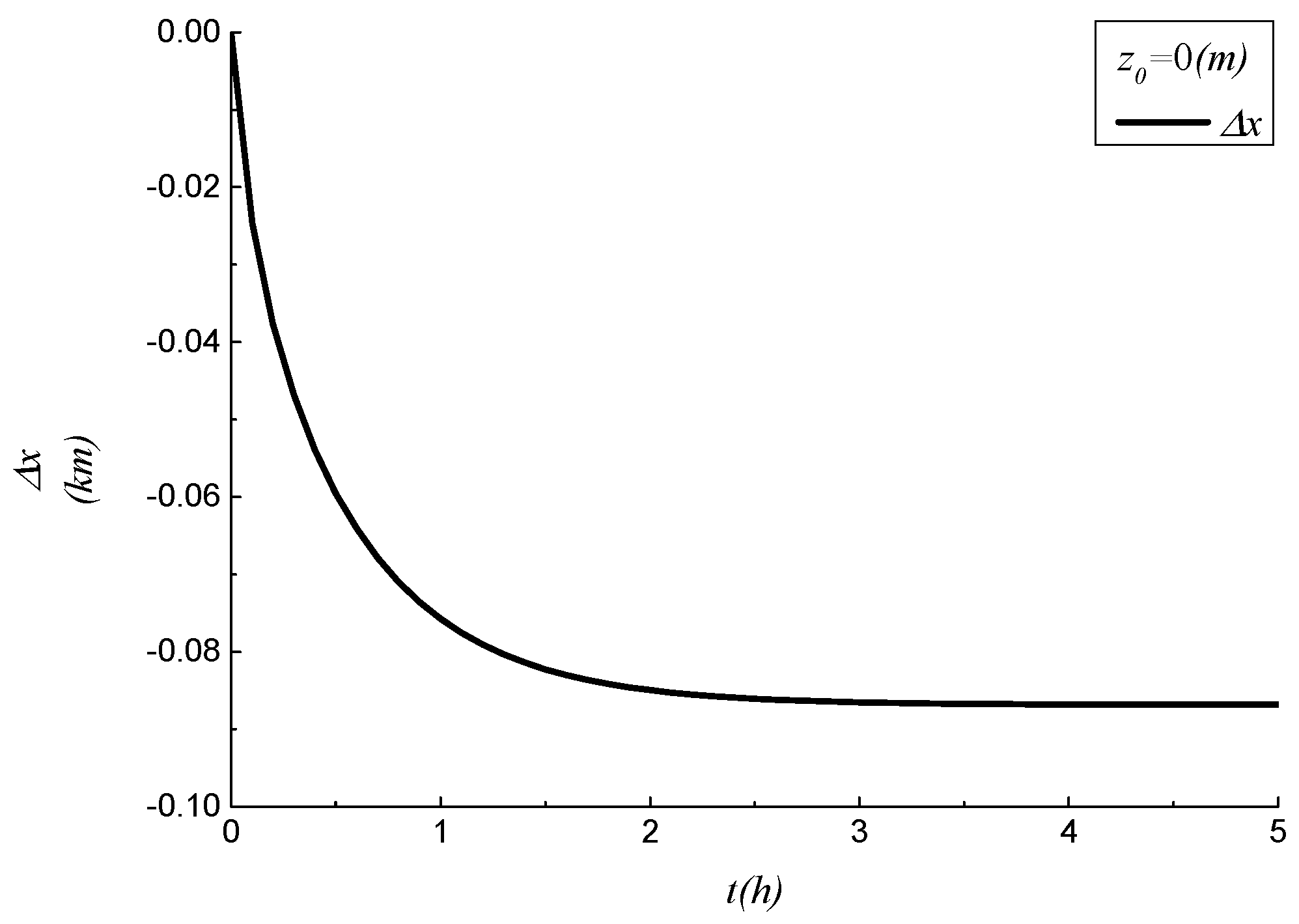
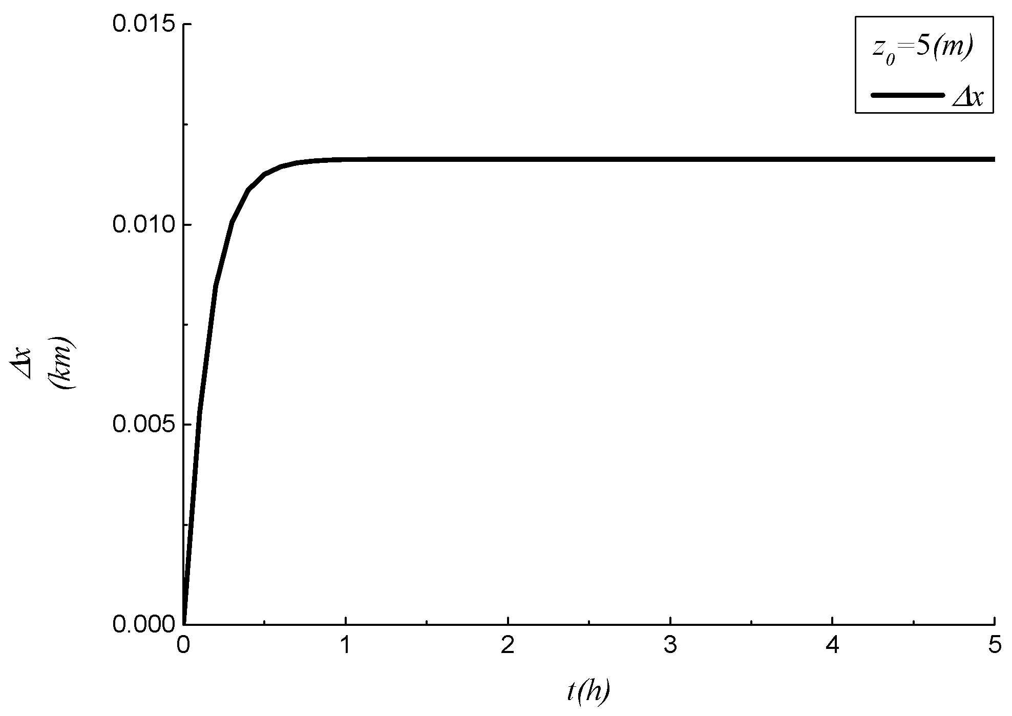
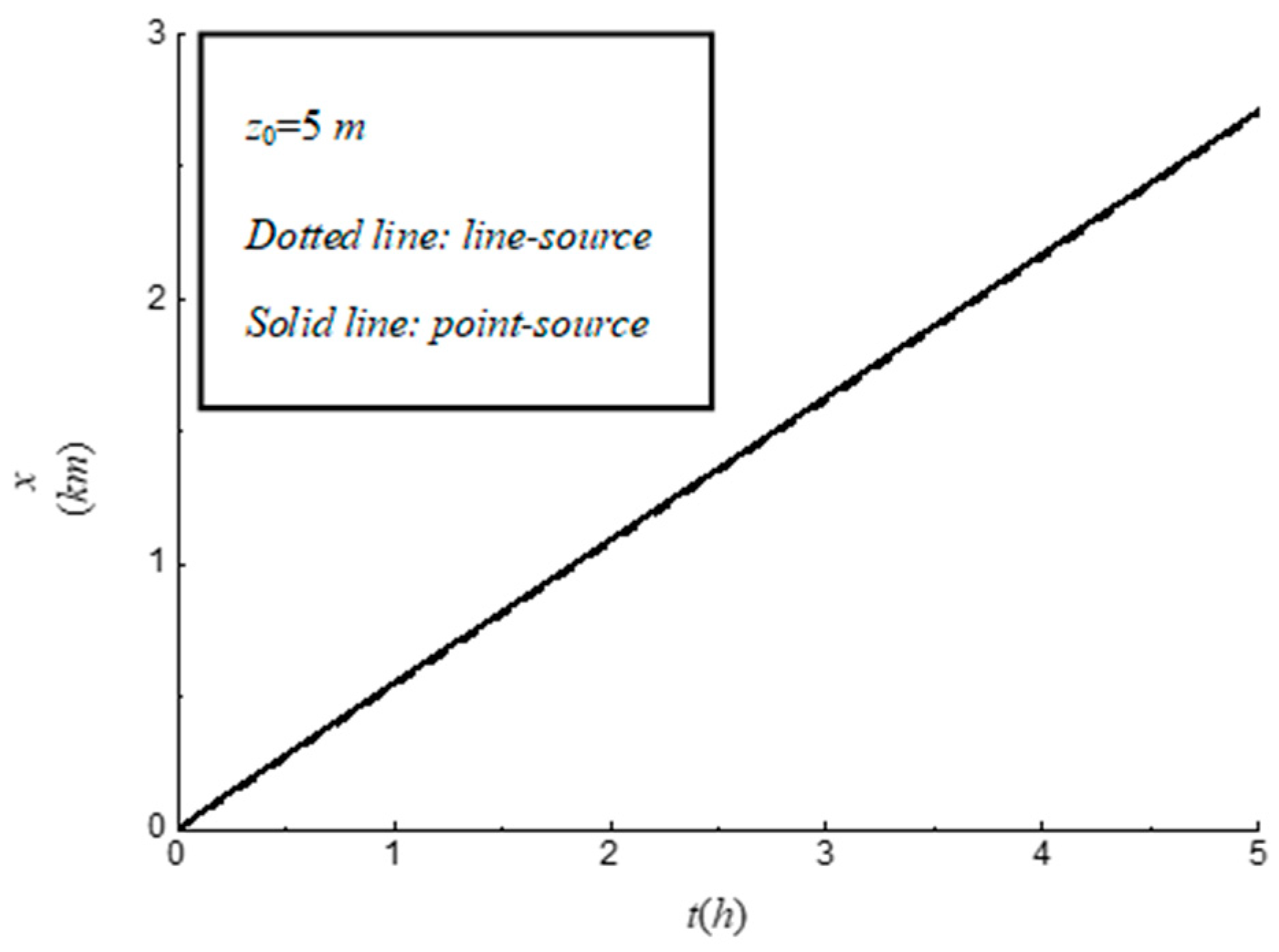
• Under the specified engineering parameters, the movement pattern of the instantaneously released point-source solute centroid was determined. This reveals that the time needed for the released point-source solute to have a downstream environmental–ecological impact on the river is dependent on the initial release location. This finding not only aligns with the conclusions drawn in the relevant literature but also offers a more extensive range of numerical results.

In summary, the analysis and results of this study not only establish the groundwork for theoretical research on more complex three-dimensional water environmental flow models but also provide a theoretical basis for engineering computations.

References

1. Tang, H. Logic mechanism and key path of developing new quality productivity to enhance water security capacity. China Water Resour. 2024, 8, 1–5. (In Chinese) [Google Scholar]
2. Gao, J. Water conservancy construction and sustainable economic and social development. J. China Inst. Water Resour. Hydropower Res. 2004, 2, 81–87. (In Chinese) [Google Scholar]
3. Peng, Q. Analysis of key problems in ecological environment monitoring. Leather Prod. Environ. Prot. Sci. Technol. 2023, 4, 38–40. (In Chinese) [Google Scholar]
4. Liu, Y. 2022 China’s Modern Ecological Development Index 70.1 Water Pollution as the Biggest Concern. Xiaokang 2022, 16, 44–45. (In Chinese) [Google Scholar]
5. Taylor, G. Dispersion of soluble matter flowing slowly through a tube. Proc. R. Soc. London. Ser. A Math. Phys. Sci. 1953, 219, 186–203. [Google Scholar]
6. Pan, M.; Meng, X. Monitoring of the relationship between water quality and point source pollution in watersheds. Environ. Sci. Res. 2000, 13, 61–64. (In Chinese) [Google Scholar]
7. Chen, Y.; Pang, Y.; Li, C.; Cui, X. Simulation study on the influence of buildings on the diffusion of atmospheric pollutants from elevated point sources. J. Environ. Eng. 2010, 4, 147–150. (In Chinese) [Google Scholar]
8. Gao, R.; Fu, X.; Wu, Z. Indicators for evaluating uncertainties of solute concentration prediction in wetland flows. Ecol. Indic. 2019, 105, 688–699. [Google Scholar] [CrossRef]
9. Huang, Z.; Shen, L.; Chen, H.; Huang, Z. Instantaneous point source and continuous source transport and diffusion with the stream. China Navig. 2020, 43, 97–100. (In Chinese) [Google Scholar]
10. Whitaker, S. The Method of Volume Averaging, Theory and Application of Transport in Porous Media; Springer: Berlin/Heidelberg, Germany, 1999. [Google Scholar]
11. Liu, S.; Masliyah, H. Dispersion in Porous Media, Handbook of Porous Media; CRC Press: Boca Raton, FL, USA, 2005. [Google Scholar]
12. Zeng, L. Analytical Study on Environmental Dispersion in Wetland Flow. Ph.D. Thesis, Peking University, Beijing, China, 2010. (In Chinese). [Google Scholar]
13. Wu, Z. Two-Scale Perturbation Analysis of Typical Taylor Dispersion Process. Ph.D. Thesis, Peking University, Beijing, China, 2014. (In Chinese). [Google Scholar]
14. Chen, G.; Zeng, L.; Wu, Z. An ecological risk assessment model for a pulsed contaminant emission into a wetland channel flow. Ecol. Model. 2010, 221, 2927–2937. [Google Scholar] [CrossRef]
15. Aris, R. On the dispersion of a solute in a fluid flowing through a tube. Proc. Roy. Soc. Lond. Ser. A-Math. Phys 1956, 235, 67–77. [Google Scholar]
16. Barton, N. On the method of moments for solute dispersion. J. Fluid Mech. 1983, 126, 205–218. [Google Scholar] [CrossRef]
17. Fu, X.; Gao, R.; Wu, Z. Additional longitudinal displacement for contaminant dispersion in wetland flow. J. Hydrol. 2016, 532, 37–45. [Google Scholar] [CrossRef]
18. Gao, R.; Fu, X.; Wu, Z.; Wang, P. Effect of release location on solute dispersion characteristics of point source in open channel wetland flow. J. Appl. Basic Eng. Sci. 2018, 26, 455–470. (In Chinese) [Google Scholar]
19. Zhou, M. Mathematical Methods for Physics; Higher Education Press: Beijing, China, 2008. (In Chinese) [Google Scholar]
20. Gu, Q. Mathematical Methods for Physics; Science Press: Beijing, China, 2012. (In Chinese) [Google Scholar]
Figure 1. Model of single-point-source solute instantaneous release. The inverted triangle at the top, represents Horizontal plane, namely Reference point for height measurement; and diagonal lines at the bottom, represents the boundary of the channel.
Sustainability 16 06912 g001
Figure 2. Model of multi-point-source solute instantaneous release.
Sustainability 16 06912 g002
Figure 3.x-t curve of movement of point-source solute centroid (z0 = 0 m).
Sustainability 16 06912 g003
Figure 4.x-t curve of movement of point-source solute centroid (z0 = 5 m).
Sustainability 16 06912 g004
Figure 5. Total displacement x of the solute centroid over time t (z0 = 0 m).
Sustainability 16 06912 g005
Figure 6. Total displacement x of the solute centroid over time t (z0 = 5 m).
Sustainability 16 06912 g006