Article

Probabilistic Prediction Model for Expressway Traffic Noise Based on Short-Term Monitoring Data

1
School of Automobile and Transportation Engineering, Guangdong Polytechnic Normal University, Guangzhou 510450, China
2
School of Civil and Transportation Engineering, Guangdong University of Technology, Guangzhou 510006, China
3
School of Mechatronic Engineering, Guangdong Polytechnic Normal University, Guangzhou 510450, China
*
Author to whom correspondence should be addressed.
Sustainability 2024, 16(16), 6841; https://doi.org/10.3390/su16166841
Submission received: 6 July 2024 / Revised: 4 August 2024 / Accepted: 7 August 2024 / Published: 9 August 2024
(This article belongs to the Special Issue Influence of Traffic Noise on Residential Environment)

Abstract

:
Seeking a straightforward and efficient method to predict expressway traffic noise, this study selected three expressway segments in Guangdong Province, China and conducted noise monitoring at ten different sites along these expressways. Data analysis revealed that the mean sound levels and standard deviations were significantly positively and negatively correlated with traffic volume, respectively, and the frequency distribution of sound levels closely resembled a normal distribution. A probability prediction model for expressway traffic noise, based on a normal distribution, has been constructed utilizing these characteristics. The mean and standard deviation of the model were determined using a linear regression method, and the relationship between the mean, standard deviation, and various noise evaluation indices was derived from the characteristics of the normal distribution. The proposed model enables the direct prediction of the statistical frequency distribution of sound levels and various noise evaluation indices. Despite using only two five-minute segments of monitoring data for training, the model’s average prediction error for Leq, L10, L50, and L90 was only 1.06, 1.07, 1.04, and 1.32 dB(A). With increased sample data for modeling, the model’s predictive accuracy notably improved. This study provides a highly effective predictive tool for assessing traffic noise for residents near expressways.

1. Introduction

In the context of rapid urbanization, the rapid expansion of expressway networks has emerged as a prominent characteristic of contemporary society. However, the concomitant issue of traffic noise pollution has become increasingly prominent, gravely impacting residents’ quality of life and health. Prolonged exposure to noise is associated with health issues, including cardiovascular diseases [1,2], sleep disorders [3], hearing loss [4], and psychological stress [5]. Expressways are characterized by significant traffic volumes, high speeds, and elevated noise levels [6,7]. Accurate prediction and assessment of these noise levels are crucial for developing effective noise management strategies and mitigation measures.
Traffic noise prediction models are a reliable method for assessing the extent of noise pollution on expressways. Countries have extensively researched and developed their unique traffic noise prediction models, tailored to the particular characteristics of their roads and vehicles. For example, the FHWA model promulgated by the USA [8], the CoRTN model developed by the UK [9], Germany’s RLS-19 model [10], and Japan’s ASJ model [11]. Researchers have refined these established models to better suit local roadway conditions, resulting in the development of various traffic noise prediction models for a range of applications. As an example, Lokhande et al. refined the FHWA model to facilitate traffic noise mapping [12]. Lodico and Donavan developed adjustment and calibration factors for the TNM model based on empirical measurements and analyses of traffic noise [13]. Cook et al. established a national system for traffic noise prediction employing the emission equations of the TNM model and hourly traffic flow statistics from various regions [14]. Rochat and Cubick employed the TNM model to study the impact of highway right-of-way configurations on traffic noise under mixed pavement conditions [15]. Ibili et al. employed an integrated approach combining the CoRTN model with multivariate linear regression to construct a model for assessing equivalent noise levels in urban central business districts [16]. Additionally, researchers have employed alternative modeling approaches to create specific traffic noise prediction models, including models that use a 20 s equivalent sound level metric [17,18,19], those based on artificial neural networks [20,21,22,23], and linear models with variable coefficients [24]. The studies referenced above have individually targeted a variety of road types and scenarios, yielding an array of diverse traffic noise prediction models and have achieved positive outcomes in their practical applications.
Traffic noise prediction models have proven effective for predicting expressway traffic noise. However, these models fall under the category of static prediction models, characterized by a single predictive measure and lack the capability to capture the dynamic variations of noise and the frequency distribution of sound levels. To address this limitation, dynamic traffic noise simulation methods based on microscopic traffic simulation have been introduced [25,26]. These methods integrate vehicle noise emission models, noise propagation models, and microscopic traffic simulation, thereby enabling the simulation and calculation of traffic noise with second-by-second dynamic changes. Dynamic traffic noise simulation methods have been successfully applied to forecast traffic noise in complex environments, such as intersections and roundabouts [27,28,29]. Dynamic traffic noise modeling requires microscopic traffic simulation tools, including commercial software suites like Paramics 6.0, PTV Vissim 11.0, and cellular automaton models [30], consequently increasing the computational demands and complexity associated with traffic noise prediction. In an effort to simplify dynamic traffic noise prediction, researchers have recently utilized the stochastic nature of traffic flows to develop probabilistic traffic noise prediction models [31,32]. These models can directly forecast various noise evaluation metrics and the statistical distribution of sound levels and also avoid the labor-intensive microsimulation of traffic flows.
Traffic noise is affected by numerous factors, including the impact of pavement materials on vehicle noise emissions and the role of sound barriers in reducing noise transmission [33,34,35]. These factors affect both the complexity of noise calculations and the accuracy of model predictions, making the prediction and assessment of traffic noise a task performed by professionals. The design of previous models was solely focused on the perspective of experts, whether involving static or dynamic models, and professional barriers limited their widespread application. When considered from the perspective of residents in a fixed location, noise reception points are constant, as is the attenuation of noise during propagation. At this point, traffic volume is the sole significant factor affecting noise levels. Therefore, it is possible to establish a simple prediction model of traffic noise at fixed points applicable to non-professional residents. This study aims to develop a site-specific noise probability distribution model by conducting short-term traffic noise monitoring, thus circumventing the complex calculations associated with noise emission and propagation, thereby making the model more accessible to the general public.
The remainder of this paper is structured as follows: Section 2 describes the methodology used in this study, which includes data collection, data analysis, and model construction. Section 3 focuses on the validation of the proposed model. Section 4 examines the factors influencing the model’s accuracy. Section 5 provides a comprehensive conclusion.

2. Methodology

2.1. Data Collection

To investigate the emission patterns and spatial distribution of traffic noise in the vicinity of highways and to construct a probabilistic traffic noise prediction model, we selected the Guanghe Expressway, Xuguang Expressway, and Huanzhou Road in Guangdong Province, China, as sites for our traffic noise data collection. The specific location details are presented in Table 1. The Guanghe Expressway, connecting Guangzhou and Heyuan, was chosen for data collection along its Shiba Town section. This section has an asphalt concrete surface, comprises three lanes in each direction, and imposes a maximum speed limit of 120 km/h. Noise monitoring stations were established at distances of 10, 50, and 100 m from the road’s edge, designated as P1, P2, and P3, respectively, with P2 partially obscured by sparse vegetation. Monitoring occurred from 8:00 AM to 10:00 AM.
Huanzhou Road, situated in Guangzhou’s Baiyun District, is a significant urban thoroughfare, with the monitored section distanced from intersections, representing a free-flow segment. This section possesses an asphalt concrete surface, includes three lanes in each direction, and has a maximum speed limit of 80 km/h. Noise monitoring points were located at 20, 5, and 10 m from the road edge, respectively, identified as P4, P5, and P6, with P6 also obstructed by sparse vegetation. Monitoring was conducted from 7:30 AM to 9:20 AM.
The Xuguang Expressway, linking Xuchang and Guangzhou, was selected for data collection along the Jianggao Town section. This segment, an asphalt concrete road, accommodates four lanes in each direction and maintains a maximum speed limit of 100 km/h. Noise monitoring points were positioned at distances of 100, 50, 20, and 15 m from the road edge, bearing identifiers P7 to P10, where P9 is shielded by a 0.5 m high solid roadside barrier, and P10 by a 3 m high roadside sound barrier. Monitoring sessions were split into two intervals: from 6:30 AM to 7:25 AM and from 3:00 PM to 3:50 PM.
During traffic noise monitoring, measures were taken to minimize interference from extraneous noise sources to the greatest extent possible. All monitoring points were situated at a height of 1.5 m above the ground, and an AWA6228 sound level meter was employed to capture the A-weighted instantaneous sound level at one-second intervals. Additionally, cameras documented the traffic conditions on the road, and manual counting was utilized to tally the traffic volume during each monitoring period. Traffic volumes and noise monitoring parameters were logged at five-minute intervals, resulting in 24 datasets for the Guanghe Expressway, 22 for Huanzhou Road, and 21 for the Xuguang Expressway.

2.2. Data Analysis

Table 2, Table 3 and Table 4 display the traffic volume and associated traffic noise data for each monitoring location. The sound level meter captures the instantaneous sound level at one-second intervals, resulting in 300 instantaneous sound level readings every five minutes for each monitoring location. In the table, μ signifies the mean sound level for the given time interval, and σ represents the standard deviation of the sound level for that interval. The traffic survey results for the three road segments consistently demonstrate a morning progression of traffic flow from low to high. Furthermore, the survey period for the Xuguang Expressway encompasses instances of elevated traffic flow in the afternoon. Despite the limited monitoring duration for each road segment, the fluctuations in traffic volume during the monitored intervals were significant, and the monitoring results adequately reflect the variations in traffic noise under diverse traffic volume conditions, rendering the data appropriate for analyzing traffic noise characteristics and for developing noise prediction models.
The data in Table 2, Table 3 and Table 4 illustrate that under identical obstacle conditions, the mean sound level (μ) decreases as the distance increases. According to the linear sound source attenuation theory, doubling the propagation distance results in a 3 dB(A) reduction in sound level; however, data from certain monitoring points do not fully conform to this rule. For instance, at monitoring points P7 and P8, the observed difference in sound levels is approximately 1 dB(A). This discrepancy may be attributed to the fact that the highway pavement is elevated 2–3 m above the noise monitoring points. This height difference provides some shielding from the noise, which is more pronounced at closer monitoring points and less affects those at greater distances.
Prior research has indicated that traffic noise escalates with increasing traffic volume, while the standard deviation of sound levels decreases as traffic volume expands [32]. The monitoring data from the current study corroborate this pattern. Figure 1 illustrates the relationship between the mean sound level, standard deviation, and traffic flow at monitoring point P1. It is apparent that a significant positive correlation exists between the mean sound level and traffic flow, as indicated by a correlation coefficient (p) of 0.915. Concurrently, the standard deviation of sound levels exhibits a significant negative correlation with traffic flow, evidenced by a correlation coefficient (p) of −0.902. Despite variations in distances and obstruction conditions, data from additional monitoring points similarly display these characteristics.
For each traffic noise dataset collected at the monitoring points, consisting of 300 instantaneous sound level readings taken over a 5 min period, a frequency distribution was calculated. The findings suggest that the majority of datasets displayed frequency distributions that closely approximated a normal distribution. Figure 2 depicts the sound level frequency distribution and the fitted normal distribution curve for monitoring point P1 during the 8:00–8:05 AM period, showing that the normal distribution curve closely matches the frequency distribution.
The Jarque–Bera test was applied to assess the normality of each dataset, indicating that out of all 222 datasets, 115 datasets passed the normality test, with a pass rate of 51.8%. To extend the analysis, each dataset was fitted to a normal distribution and the coefficient of determination R2 for the fits was calculated. These outcomes are illustrated in Figure 3. The traffic noise monitoring data from the Xuguang Expressway demonstrated the closest fit to a normal distribution, with an average R2 of 0.911 and 92.5% of R2 values exceeding 0.8. R2 values for traffic noise data from the Guanghe Expressway and Huanzhou Road were generally similar, where the Guanghe Expressway had an average R2 of 0.861, with 79.2% of R2 values exceeding 0.8, and Huanzhou Road had an average R2 of 0.847, with 78.8% of R2 values exceeding 0.8. The mean R2 for the 115 datasets meeting the normality criteria was 0.898, whereas for the 107 datasets not meeting these criteria, it was 0.865. This suggests that even the datasets not meeting the normality criteria exhibited a substantial fit to a normal distribution, consistent with the characteristics of a normal distribution.
The above is a preliminary analysis of the data with a 5 min statistical period, confirming three key observations: (a) there is a robust positive correlation between the average sound level and traffic flow, (b) there is a robust negative correlation between the standard deviation of the sound level and traffic flow, and (c) the frequency distribution of sound levels approximates a normal distribution.

2.3. Model Development

Based on the preceding analysis, a probability distribution model can be established for traffic noise at each monitoring point, utilizing a normal distribution model to characterize the distribution of sound levels across different traffic volumes. The mean and standard deviation of the normal distribution model are derived from the traffic volume, with a linear regression model employed to delineate the relationship between the logarithm of traffic volume and the mean sound level, as well as between traffic volume and the standard deviation.
Prior to model construction, it is imperative to remove any outlier data. Avoiding interference from extraneous noises during traffic noise monitoring, such as abrupt background noise, unforeseen vehicle honking, and animal vocalizations, is challenging, which can contaminate the routine monitoring data, resulting in atypical means or standard deviations of sound levels. Employing the logarithm of traffic volume as the independent variable and the mean sound level as the dependent variable, linear regression analysis is performed on the entire dataset for each monitoring point, and Cook’s distance is computed between the variables to identify outliers in the dataset.
Cook’s distance quantifies the change in model parameter estimates following the exclusion of an observation and is utilized to pinpoint observations exerting substantial influence in regression analysis. An observation with a larger Cook’s distance signifies a greater impact on parameter estimation, thereby increasing the probability that the observation is an outlier. The Cook’s distance for the i-th observation is denoted as
D i = j = 1 n y ^ j y ^ j i 2 p · M S E ,
where y ^ j is the j-th fitted response value, y ^ j i is the j-th fitted response value where the fit does not include observation i, MSE is the mean squared error, and p is the number of coefficients in the regression model.
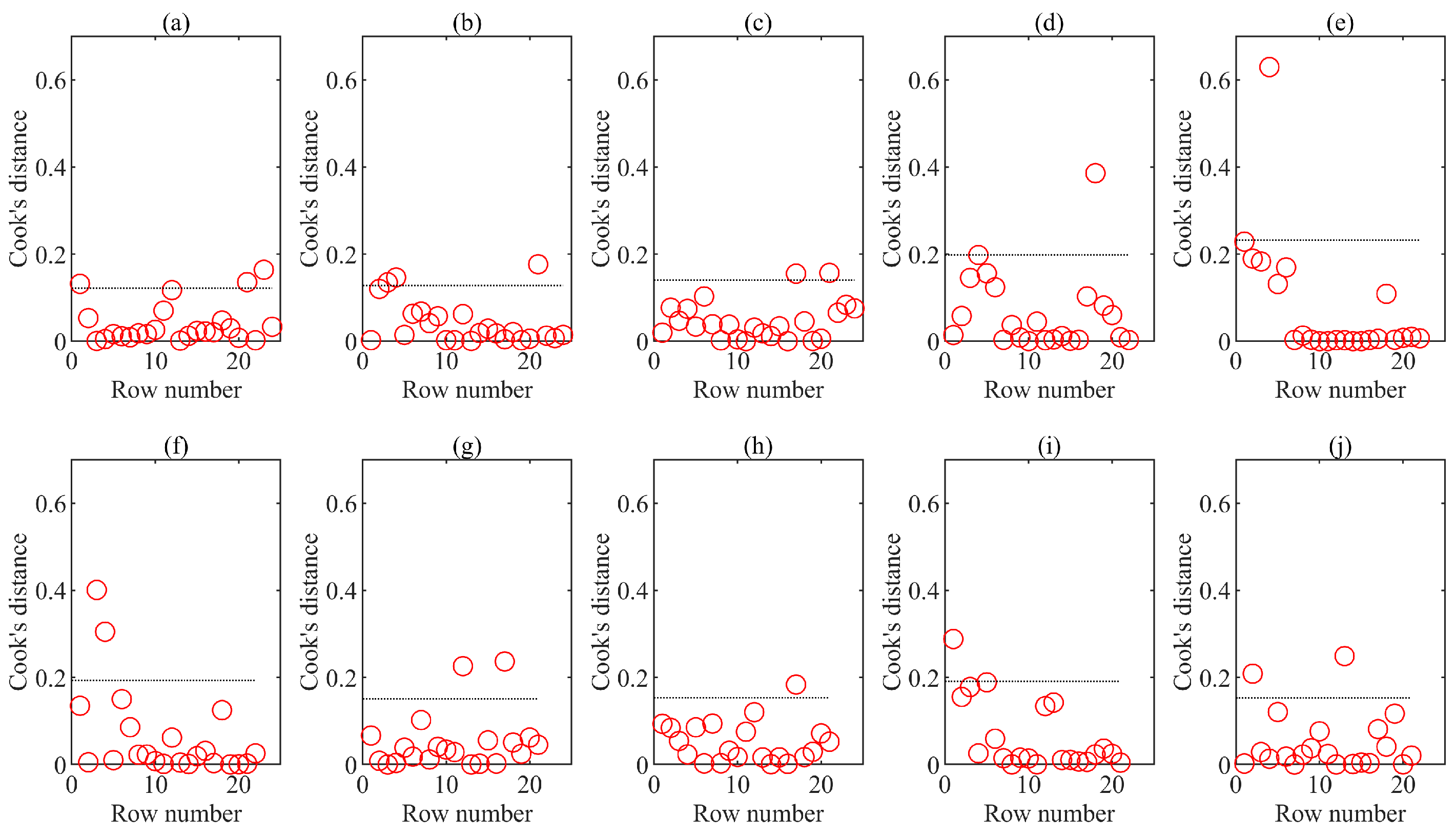
Figure 4 illustrates the Cook’s distances for the relationship between the logarithm of traffic volume (log10(Q)) and the mean sound level (μ) at each monitoring point. Observations with Cook’s distances exceeding 0.5 are considered outliers and are therefore excluded from the analysis. As a result, the fourth observation at monitoring point P5, which corresponds to the data collected during the 7:45–7:50 time interval, has been removed. In a similar analytical approach, with traffic volume (Q) as the independent variable and the standard deviation of the sound level (σ) as the dependent variable, Figure 5 displays the Cook’s distances. This analysis suggests the removal of the first observation at monitoring point P6, which represents the data gathered in the 7:30–7:35 time interval.
After the exclusion of two outlier datasets, we applied linear regression analysis to develop a probabilistic model for predicting traffic noise levels. For each monitoring point, a subset of the data was selected to derive the regression equation, while the remaining data were utilized to validate the model’s accuracy. The criteria for data selection were as follows: (a) To ensure the representativeness of the dataset for modeling purposes, the selected data should demonstrate sufficient variability in traffic volume, with the maximum volume being at least double the minimum. (b) Data were randomly chosen provided that criterion (a) was met.
Utilize the selected dataset to establish a linear regression equation between the mean sound level and log10(Q), expressed as
μ = a + b log 10 Q ,
b = i = 1 n log 10 Q i log 10 Q ¯ μ i μ ¯ i = 1 n log 10 Q i log 10 Q ¯ 2 ,
and
a = μ ¯ b log 10 Q ¯ ,
where n represents the number of samples selected, and n 2 . Similarly, the standard deviation of sound levels (σ) can be derived in relation to traffic flow (Q) as
σ = c + d Q ,
d = i = 1 n Q i Q ¯ σ i σ i = 1 n Q i Q ¯ 2 ,
and
c = σ ¯ d Q ¯ .
The model determines the mean sound level (μ) and standard deviation (σ) at the noise observation point based on traffic volume. It assumes that the statistical distribution of sound levels at the observation point follows a normal distribution. By utilizing the properties of the normal distribution, the statistical sound level assessment indicators can be calculated as
L 10 = μ + 1.28 σ ,
L 50 = μ ,
L 90 = μ 1.28 σ .
The equivalent sound level Leq is obtained as a noise evaluation metric according to the principle of averaging acoustic energy. Within the framework of a normal distribution model, we integrate based on the energy ratio of the sound levels, deriving the relationship between Leq and the parameters μ and σ as
L e q = μ + 0.115 σ 2 .
The specific derivation process is as follows:
L e q = 10 log 10 10 0.1 x · 1 σ 2 π · e x p x μ 2 2 σ 2 d x = 10 log 10 1 σ 2 π · e x p μ 2 2 σ 2 e x p 1 2 σ 2 x 2 + μ σ 2 + 0.1 · ln 10 x d x .
According to the Gauss integral formula, we have
e x p a x 2 + b x d x = π a · e x p b 2 4 a .
Let a = 1 2 σ 2 , and b = μ σ 2 + 0.1 · ln 10 , therefore,
10 log 10 1 σ 2 π · e x p μ 2 2 σ 2 e x p 1 2 σ 2 x 2 + μ σ 2 + 0.1 · ln 10 x d x = 10 log 10 1 σ 2 π · e x p μ 2 2 σ 2 · π 1 2 σ 2 · e x p μ σ 2 + 0.1 · ln 10 2 4 2 σ 2 = 10 log 10 e x p μ 2 2 σ 2 · e x p μ 2 2 σ 2 + 1 2 · σ 2 · 0.1 2 · ln 10 2 + μ · 0.1 · ln 10 = μ + 0.115 σ 2 .

3. Model Validation

To evaluate the model’s accuracy and reliability, we examine the most extreme scenarios by selecting merely two data points (n = 2 in Equations (3) and (6)) from each monitoring site to establish the model. This entails using only two data points to determine the four parameters, a, b, c, and d in Equations (2) and (5), with the remaining data utilized for model validation. During model verification, we use the actual measured traffic volume (Q) to substitute into Equations (2) and (5) to obtain the μ and σ of the sound level distribution. Subsequently applying Equations (8)–(11), we calculate the predicted values of various noise evaluation indices, which are then compared with the corresponding measured values.
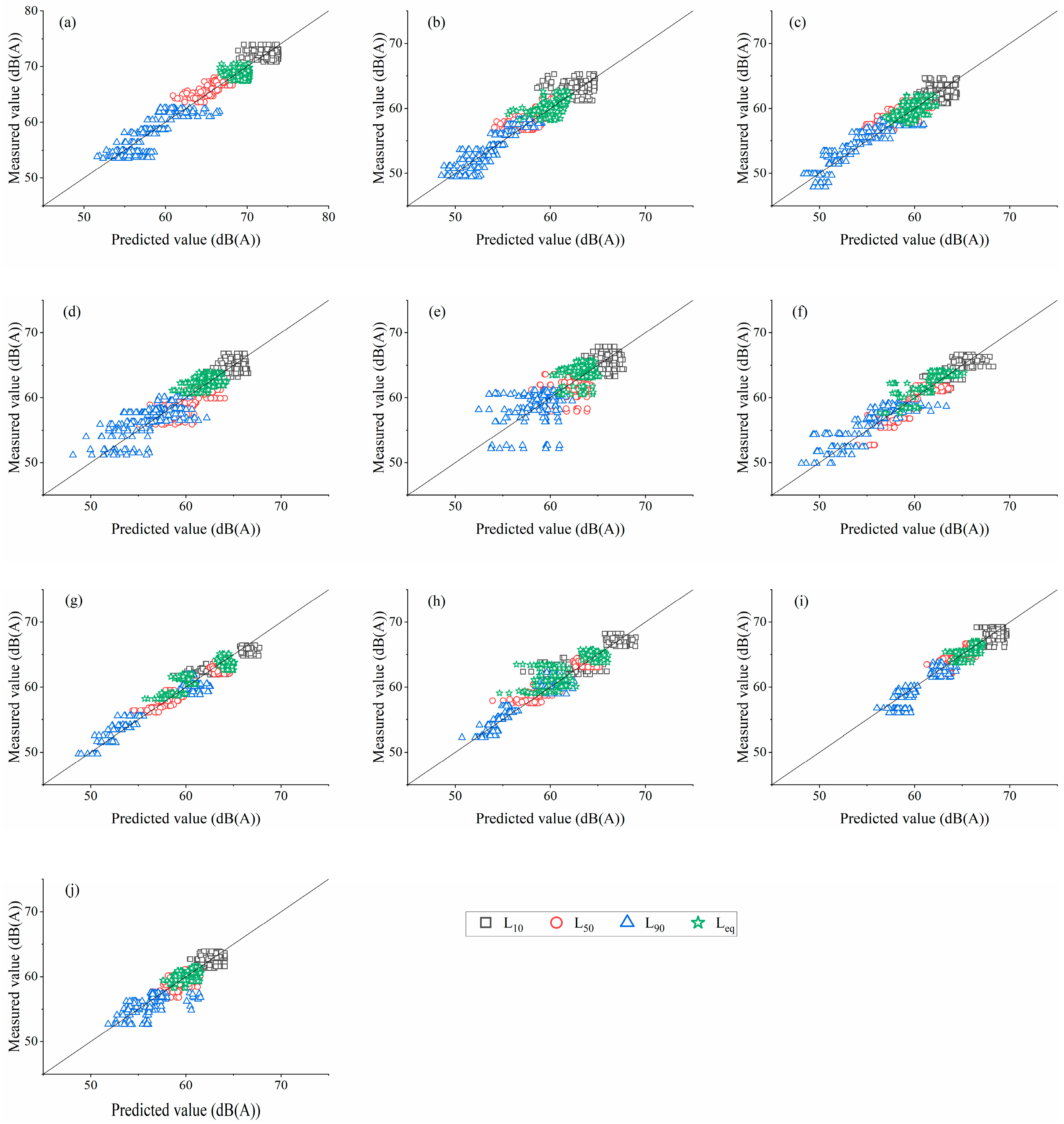
Utilizing the aforementioned method, each monitoring point underwent 10 random tests, and comparisons were drawn between all predicted and measured noise evaluation indices. The results depicted in Figure 6 reveal that the predicted values of the noise evaluation indices correspond closely to the measured values, with the scatter points evenly distributed about the y = x line, suggesting a minimal systematic error in the model. Variations in Leq, L10, and L50 are typically not exceeding 8 dB(A), and the model demonstrates minor prediction error for these indices. The variation in L90 is more pronounced, surpassing 10 dB(A) at all monitoring points with the exception of P10. The model exhibits a greater prediction error for L90 compared to other indices, particularly at monitoring points P4 and P5. This is attributed to L90 representing the background noise, with Huanzhou Road, corresponding to P4 and P5, being a major urban thoroughfare with intermittent pedestrian and non-motorized vehicle traffic in proximity to the monitoring points, resulting in substantial interference with the background noise. Regarding Guanghe Expressway and Xuguang Expressway, monitoring points P3 and P7, respectively, demonstrated superior data alignment. These monitoring points, located at a distance of 100 m from the highway, exhibit more stable monitoring data with fewer fluctuations. Notably, monitoring points P9 and P10, which feature sound barriers of different heights, result in an attenuation of noise due to obstacles, leading to a narrower sound level distribution, which manifested as a reduced standard deviation. The model retains high predictive accuracy for such monitoring points, as illustrated in Figure 6i,j.
A statistical analysis of the model error for all monitoring points is depicted in Figure 7. The prediction accuracy of the model for Leq, L10, and L50 indices is comparable. The mean absolute deviation (MAD) for L10 is 1.07 dB(A), exhibiting a maximum deviation of 5.04 dB(A), and 95% of deviations fall within 2.63 dB(A); the MAD for L50 is 1.04 dB(A), exhibiting a maximum deviation of 6.07 dB(A), and 95% of deviations fall within 2.69 dB(A); the MAD for Leq is 1.06 dB(A), exhibiting a maximum deviation of 6.86 dB(A), and 95% of deviations fall within 2.64 dB(A). Considering a prediction deviation for Leq exceeding 3.0 dB(A) as a model failure, the model’s failure rate stands at a mere 3.35%. The prediction deviation for L90 is more substantial, with a MAD of 1.32 dB(A), a maximum deviation of 8.86 dB(A), and 95% of deviations falling within 3.36 dB(A). This suggests that background noise is susceptible to disturbance from various factors, exhibits significant randomness, and poses challenges for accurate prediction.
These findings suggest that the model’s predicted values closely correspond to the measured values, and even with the establishment of the model based on merely two data points at each monitoring point, the model retains high predictive accuracy. Consequently, provided that noise monitoring occurs once during periods of low and high traffic flow, each exceeding 5 min, a highly accurate traffic noise prediction probability model can be developed.

4. Discussion

4.1. The Influence of Modeling Samples on Model Accuracy

Upon further increasing the sample size for model construction, we assessed the variations in model error. Each monitoring point utilizes between two and twelve actual measured samples for constructing the model (n = 2, 3, …, 12 in Equations (3) and (6)), and each model underwent 10 random tests, with both mean and maximum errors being recorded, as depicted in Figure 8. As the sample size of the modeling data increased, the mean absolute errors and the maximum errors of the various noise evaluation indices demonstrate a discernible downward trend. Due to the stochastic nature of the modeling data selection, the error trajectories do not uniformly decrease but instead display irregular fluctuations. The mean errors associated with the noise evaluation indices at each monitoring point approximate 1 dB(A), with the L90 deviations at monitoring points P4 and P5 being marginally higher than those of other indices, reaching approximately 2 dB(A), which is in agreement with the findings depicted in Figure 6. The range of maximum deviations for the noise evaluation indices at each monitoring point differs, with monitoring points P1, P3, P4, P9, and P10 exhibiting reduced deviations, declining from roughly 3 dB(A) to approximately 2 dB(A). It is noteworthy that L90 is the evaluation index with the most significant deviation, which is an expected observation given the high variability inherent in L90. Nonetheless, a minority of monitoring points exhibit the largest deviations in Leq, such as P6 and P8, with maximum deviations reaching 5–6 dB(A), suggesting that the data for P6 and P8 may include several outliers.
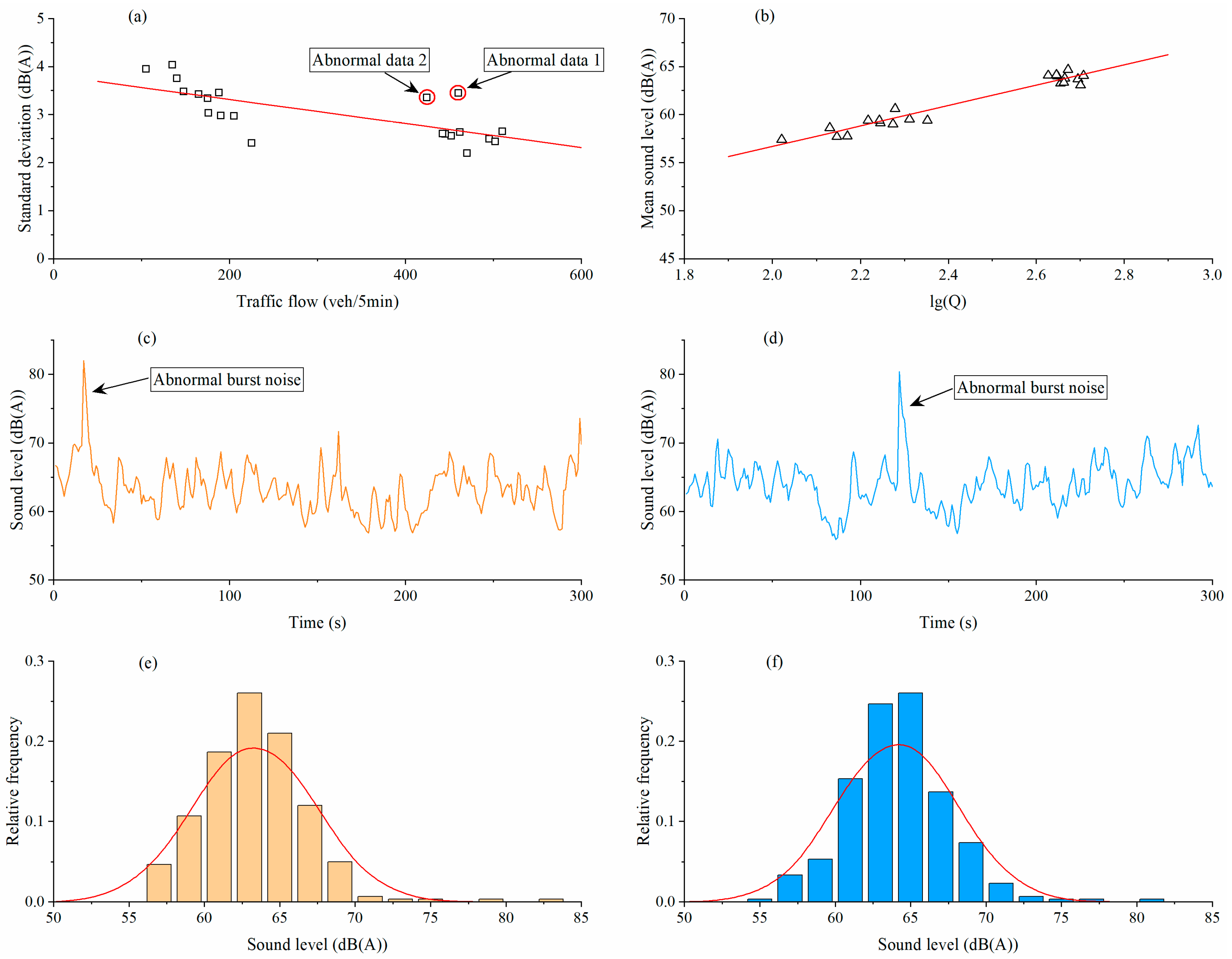
An analysis was conducted of the actual measurement dataset from monitoring point P8, which exhibited larger errors, as illustrated in Figure 9. A strong linear relationship exists between the mean sound level μ and Log10(Q), with no discernible outliers (Figure 9b). However, in the scatter plot showing the standard deviation of the sound level (σ) and traffic volume (Q), a few outliers are present that significantly deviate from the trend line (Figure 9a). Upon examination of the time series of these outliers, it was observed that each exhibited high-amplitude impulsive noise events, with peaks exceeding 80 dB(A), which surpass the regular noise levels by more than 10 dB(A) (Figure 9c,d). These impulsive noise events typically last for 2–3 s and are likely attributable to sudden vehicle honking. On highways, vehicle honking is an occasional occurrence and is part of traffic noise, which is difficult to avoid in noise monitoring. The sporadic nature of vehicle honking can compromise the accuracy of traffic noise prediction models. The impulsive noise has a negligible impact on the mean sound level and the frequency distributions of sound levels, as depicted in Figure 9e,f; the frequency distributions of the two anomalous data samples continue to follow a normal distribution. However, these high-amplitude impulsive noise events increase the equivalent continuous sound level (Leq) and the standard deviation (σ), resulting in diminished predictive accuracy of the model.

4.2. Applicability and Limitations of the Model

In comparison with established traffic noise prediction models, such as the static and dynamic models, the proposed model presents several advantages: (a) It is based on actual measurement data, thereby obviating the need for calculating vehicle noise emissions and complex noise propagation attenuation. (b) It enables a direct prediction of commonly used noise assessment indices (Leq, L10, L50, and L90). While dynamic models also provide similar functionality, these indices are obtained indirectly rather than directly. (c) The processes of modeling and calculation in this model are straightforward, rendering it more user-friendly for non-expert environmental noise managers.
Based on the above advantages, the proposed model has potential application in noise-sensitive areas near large arterial roads, where long-term noise monitoring is not available. The model is also applicable to noise prediction and assessment for ordinary residents in their homes. In the absence of long-term monitoring equipment, short-term traffic and noise data may be utilized to predict noise pollution indicators under varying traffic conditions. The operational process comprises the following five steps: (a) Collect at least two sets of 5 min traffic volume and noise data under different traffic volume conditions, as at least two samples are required to establish the regression equation. (b) Calculate the mean and standard deviation of the noise levels. (c) Build a regression model using Equations (2)–(7). (d) Predict the mean and standard deviation of noise levels at other traffic volume states. (e) Calculate various noise evaluation indices using Equations (8)–(11).
Nevertheless, the model also presents notable limitations. For instance, the model is limited to single-point predictions and requires re-modeling with fresh monitoring data for different prediction distances. Additionally, the model does not account for the impact of varying vehicle type proportions, and significant changes in the proportion of large vehicles will increase the model’s error. Furthermore, this model assumes a normal distribution, and relies on data exclusively collected from highways and urban main roads in a free-flow state, potentially leading to errors when applied to roads in non-free-flow states. Finally, it is important to note that studies indicate that when the hourly traffic volume exceeds 400 vehicles, the associated traffic noise approximates a normal distribution [32]. This method is therefore applicable only when the 5 min traffic volume exceeds 34 vehicles.
Theoretically, an increased number of data samples employed in modeling correlates with enhanced precision of the model, yet the core objective of this study is to devise a robust traffic noise prediction model utilizing minimal short-term monitoring data. For example, only two instances of five-minute noise monitoring sessions are adequate to accurately forecast the noise distribution across varying traffic flow conditions. Should there be a substantial volume of monitoring data that comprehensively encompasses diverse traffic flow conditions, then such single-point-centric prediction models may become redundant.

5. Conclusions

The analysis of highway traffic noise monitoring data indicates that a significant linear relationship exists between traffic volume, mean noise levels, and their standard deviations. Furthermore, the frequency distribution of traffic noise at the monitoring points closely resembles a normal distribution. Drawing on these observations, this study proposes a probabilistic model for the prediction of highway traffic noise utilizing monitoring data. The model enables a direct prediction of the noise distribution across a range of traffic volumes and commonly employed noise evaluation indices. Upon evaluation, with merely two five-minute real-world samples, the model consistently demonstrates high predictive accuracy. The methodology proposed in this study is characterized by its straightforward modeling approach, high accuracy in noise prediction, and the capacity to simultaneously predict multiple noise evaluation indices, possessing potential for application in both predicting and managing highway noise environments.

Author Contributions

Conceptualization, Z.L.; methodology, F.L.; validation, H.W.; formal analysis, C.D.; investigation, Z.L.; data curation, F.Y.; writing—review & editing, Y.R.; visualization, Z.L.; funding acquisition, F.L. All authors have read and agreed to the published version of the manuscript.

Funding

This research was funded by the Research Capacity Enhancement Project for Universities Building Doctoral Programs in Guangdong Province (No. 22GPNUZDJS45 and 22GPNUZDJS44); the National Environmental Protection Engineering and Technology Center for Road Traffic Noise Control; the Key Research Projects of Higher Education Institutions of Guangdong Provincial Department of Education (2023); the Special Initiative for Priority Areas at General Higher Education Institutions in Guangdong Province, China (No. 2023ZDZX3009); and the Dynamic Calculation of Road Traffic Noise Distribution and Spatial Layout Optimization (No. 2023SDKYA021).

Institutional Review Board Statement

Not applicable.

Informed Consent Statement

Not applicable.

Data Availability Statement

The data that support the findings of this study are available on request from the corresponding author upon reasonable request.

Conflicts of Interest

The authors declare no conflicts of interest regarding the publication of this paper.

References

  1. Cole-Hunter, T.; So, R.; Amini, H.; Backalarz, C.; Brandt, J.; Bräuner, E.V.; Hertel, O.; Jensen, S.S.; Jørgensen, J.T.; Ketzel, M.; et al. Long-term exposure to road traffic noise and all-cause and cause-specific mortality: A Danish Nurse Cohort study. Sci. Total Environ. 2022, 820, 153057. [Google Scholar] [CrossRef] [PubMed]
  2. Gu, T.; Yang, T.; Wang, J.; Hu, X.; Xu, Z.; Wang, Y.; Jin, J.; Zhang, J.; He, T.; Li, G.; et al. Modification of green space on the associations between long-term road traffic noise exposure and incident intracerebral hemorrhage: A prospective cohort study. Environ. Res. 2023, 231, 116189. [Google Scholar] [CrossRef]
  3. Smith, M.G.; Younes, M.; Aeschbach, D.; Elmenhorst, E.M.; Müller, U.; Basner, M. Traffic noise-induced changes in wake-propensity measured with the Odds-Ratio Product (ORP). Sci. Total Environ. 2022, 805, 150191. [Google Scholar] [CrossRef] [PubMed]
  4. Natarajan, N.; Batts, S.; Stankovic, K.M. Noise-Induced Hearing Loss. J. Clin. Med. 2023, 12, 2347. [Google Scholar] [CrossRef] [PubMed]
  5. Klompmaker, J.O.; Hoek, G.; Bloemsma, L.D.; Wijga, A.H.; van den Brink, C.; Brunekreef, B.; Lebret, E.; Gehring, U.; Janssen, N.A.H. Associations of combined exposures to surrounding green, air pollution and traffic noise on mental health. Environ. Int. 2019, 129, 525–537. [Google Scholar] [CrossRef]
  6. Li, H.; Xie, H. Noise exposure of the residential areas close to urban expressways in a high-rise mountainous city. Environ. Plan. B: Urban Anal. City Sci. 2021, 48, 1414–1429. [Google Scholar] [CrossRef]
  7. Halim, H.; Abdullah, R. Equivalent noise level response to number of vehicles: A comparison between a high traffic flow and low traffic flow highway in Klang Valley, Malaysia. Front. Environ. Sci. 2014, 2, 13. [Google Scholar] [CrossRef]
  8. Fleming, G.; Rapoza, A.; Lee, C. Development of national reference energy mean emission levels for the FHWA Traffic Noise Model. In Report No FHWA-PD-96-008 and DOT- VNTSC-96-2; John A. Volpe National Transportation Systems Center: Cambridge, MA, USA, 1995. [Google Scholar]
  9. Givargis, S.; Mahmoodi, M. Converting the UK calculation of road traffic noise (CORTN) to a model capable of calculating LAeq,1h for the Tehran’s roads. Appl. Acoust. 2008, 69, 1108–1113. [Google Scholar] [CrossRef]
  10. Bartolomaeus, W. Guidelines for noise protection at roads—rls19. Larmbekampfung 2019, 14, 203–207. [Google Scholar] [CrossRef]
  11. Sakamoto, S. Road traffic noise prediction model “ASJ RTN-Model 2018”: Report of the research committee on road traffic noise. Acoust. Sci. Technol. 2020, 41, 529–589. [Google Scholar] [CrossRef]
  12. Lokhande, S.K.; Pathak, S.S.; Kokate, P.K.; Bodhe, G.L. Evaluation and forecasting of highway traffic noise in the city of Nagpur, India. Int. J. Earth Sci. Eng. 2016, 9, 1529–1535. [Google Scholar]
  13. Lodico, D.; Donavan, P. Using onboard sound intensity measurements to interpret results of traffic noise modeling. Transp. Res. Rec. 2013, 2362, 9–15. [Google Scholar] [CrossRef]
  14. Cook, M.; Gee, K.; Transtrum, M.; Lympany, S. An app for nationwide dynamic traffic noise prediction. In INTER-NOISE and NOISE-CON Congress and Conference Proceedings; NOISE-CON22; Institute of Noise Control Engineering: Grand Rapids, MI, USA, 2023; Volume 266. [Google Scholar] [CrossRef]
  15. Rochat, J.; Cubick, K. Acoustically soft ground as a highway traffic noise reduction strategy. In INTER-NOISE and NOISE-CON Congress and Conference Proceedings; Institute of Noise Control Engineering: Lexington, KY, USA, 2022; Volume 264. [Google Scholar] [CrossRef]
  16. Ibili, F.; Owolabi, A.O.; Ackaah, W.; Massaquoi, A.B. Statistical modelling for urban roads traffic noise levels. Sci. Afr. 2022, 15, e01131. [Google Scholar] [CrossRef]
  17. Pamanikabud, P.; Tansatcha, M. Simulation of highway traffic noise with utilization of equivalent sound level of pass-by vehicle. J. Acoust. Soc. Am. 2008, 123 (Suppl. S5), 3824. [Google Scholar] [CrossRef]
  18. Pamanikabud, P.; Tansatcha, M.; Brown, A.L. Development of a highway noise prediction model using an Leq20 s measure of basic vehicular noise. J. Sound Vib. 2008, 316, 317–330. [Google Scholar] [CrossRef]
  19. Zhao, J.; Ding, Z.; Hu, B.; Chen, Y.; Yang, W. Assessment and improvement of a highway traffic noise prediction model with Leq(20 s) as the basic vehicular noise. Appl. Acoust. 2015, 97, 78–83. [Google Scholar] [CrossRef]
  20. Ahmed, A.A.; Pradhan, B.; Chakraborty, S.; Alamri, A. Developing vehicular traffic noise prediction model through ensemble machine learning algorithms with GIS. Arab. J. Geosci. 2021, 14, 1564. [Google Scholar] [CrossRef]
  21. Ahmed, A.A.; Pradhan, B.; Chakraborty, S.; Alamri, A.; Lee, C.W. An Optimized Deep Neural Network Approach for Vehicular Traffic Noise Trend Modeling. IEEE Access 2021, 9, 107375–107386. [Google Scholar] [CrossRef]
  22. Huang, B.; Pan, Z.; Liu, Z.; Hou, G.; Yang, H. Acoustic amenity analysis for high-rise building along urban expressway: Modeling traffic noise vertical propagation using neural networks. Transp. Res. Part D Transp. Environ. 2017, 53, 63–77. [Google Scholar] [CrossRef]
  23. Kumar, P.; Nigam, S.P.; Kumar, N. Vehicular traffic noise modeling using artificial neural network approach. Transp. Res. Part C Emerg. Technol. 2014, 40, 111–122. [Google Scholar] [CrossRef]
  24. Rassafi, A.A.; Ghassempour, J. Highway traffic noise modeling and estimation based on vehicles volume and speed. Adv. Environ. Res. 2015, 4, 211–218. [Google Scholar] [CrossRef]
  25. Cai, M.; Li, F.; Liu, J.-K. Dynamic simulation and characteristics analysis of traffic noise at signal-controlled pedestrian crossing junction. Noise Control Eng. J. 2011, 59, 549–555. [Google Scholar] [CrossRef]
  26. Can, A.; Chevallier, E.; Nadji, M.; Leclercq, L. Dynamic traffic modeling for noise impact assessment of traffic strategies. Acta Acust. United Acust. 2010, 96, 482–493. [Google Scholar] [CrossRef]
  27. Estévez-Mauriz, L.; Forssén, J. Dynamic traffic noise assessment tool: A comparative study between a roundabout and a signalised intersection. Appl. Acoust. 2018, 130, 71–86. [Google Scholar] [CrossRef]
  28. Li, F.; Cai, M.; Liu, J.K.; Yu, Z. Dynamic traffic noise simulation at a signalized intersection among buildings. Noise Control. Eng. J. 2011, 59, 202–210. [Google Scholar] [CrossRef]
  29. Li, F.; Lin, Y.; Cai, M.; Du, C. Dynamic simulation and characteristics analysis of traffic noise at roundabout and signalized intersections. Appl. Acoust. 2017, 121, 14–24. [Google Scholar] [CrossRef]
  30. Du, C.; Qiu, X.; Li, F.; Cai, M. A simulation of traffic noise emissions at a roundabout based on a cellular automaton model. Acta Acust. 2021, 5, 42. [Google Scholar] [CrossRef]
  31. Li, F.; Liao, S.S.; Cai, M. A new probability statistical model for traffic noise prediction on free flow roads and control flow roads. Transp. Res. Part D Transp. Environ. 2016, 49, 313–322. [Google Scholar] [CrossRef]
  32. Li, F.; Xue, W.; Rong, Y.; Du, C.; Tang, J.; Zhao, Y. A probability distribution prediction method for expressway traffic noise. Transp. Res. Part D Transp. Environ. 2022, 103, 103175. [Google Scholar] [CrossRef]
  33. Cho, D.S.; Mun, S. Development of a highway traffic noise prediction model that considers various road surface types. Appl. Acoust. 2008, 69, 1120–1128. [Google Scholar] [CrossRef]
  34. Cubick, K.; Rochat, J. Solid safety barriers as a highway traffic noise reduction strategy. In INTER-NOISE and NOISE-CON Congress and Conference Proceedings; NOISE-CON22; Institute of Noise Control Engineering: Lexington, KY, USA, 2022; Volume 264. [Google Scholar] [CrossRef]
  35. Fujiwara, T.; Meiarashi, S.; Namikawa, Y.; Hasebe, M. Reduction of equivalent continuous A-weighted sound pressure levels by porous elastic road surfaces. Appl. Acoust. 2005, 66, 766–778. [Google Scholar] [CrossRef]
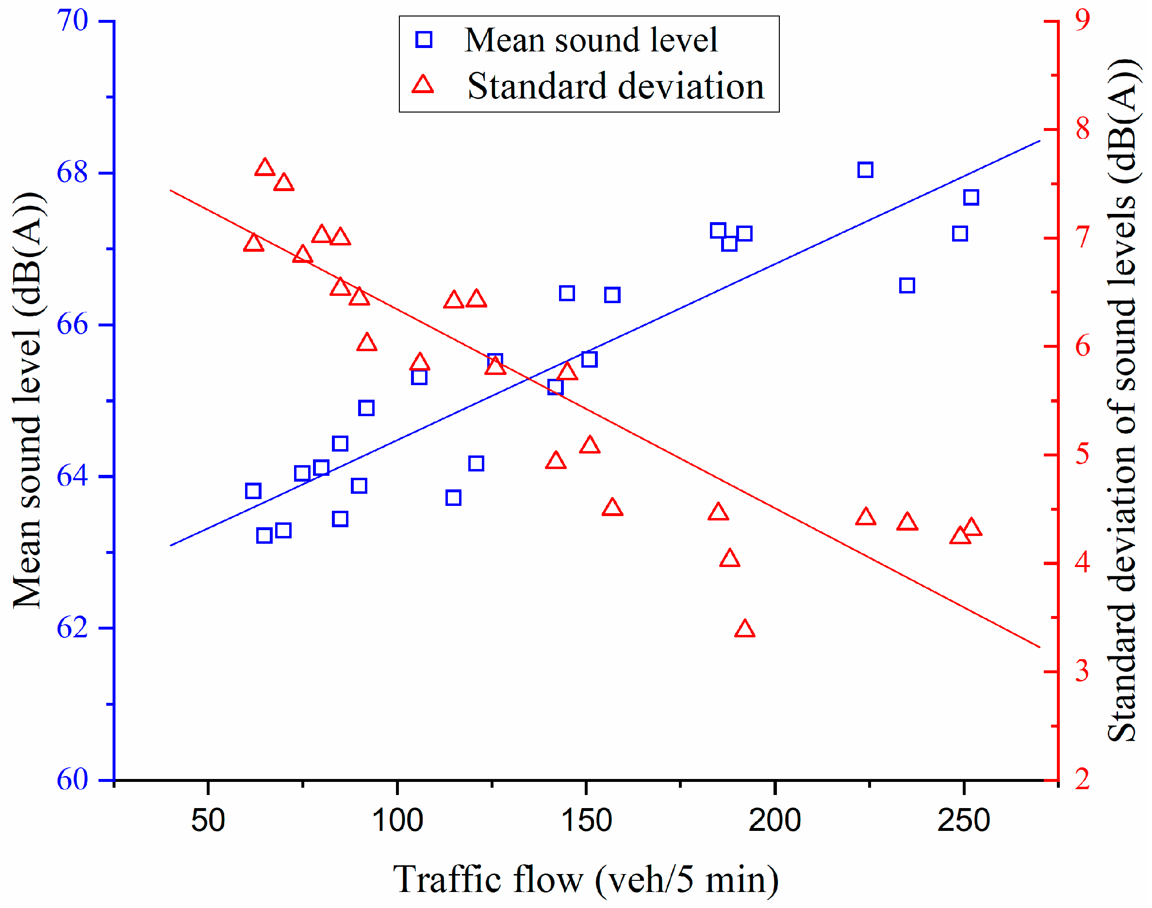
Figure 1. The relationship between mean sound level, standard deviation, and traffic volume at monitoring point P1.
Sustainability 16 06841 g001
Figure 2. Frequency distribution of sound levels at monitoring point P1 during 8:00 to 8:05 AM.
Sustainability 16 06841 g002
Figure 3. Statistical chart of the coefficient of determination R2 for normal distribution fitting. (a) Cumulative distribution of R2. (b) Box chart of R2 of Xuguang Expressway. (c) Box chart of R2 of Guanghe Expressway. (d) Box chart of R2 of Huanzhou Road.
Sustainability 16 06841 g003
Figure 4. Cook’s distance between log10(Q) and mean noise level at each monitoring point. (a) Data at P1. (b) Data at P2. (c) Data at P3. (d) Data at P4. (e) Data at P5. (f) Data at P6. (g) Data at P7. (h) Data at P8. (i) Data at P9. (j) Data at P10.
Sustainability 16 06841 g004
Figure 5. Cook’s distance between traffic volume and sound level standard deviation at each monitoring point. (a) Data at P1. (b) Data at P2. (c) Data at P3. (d) Data at P4. (e) Data at P5. (f) Data at P6. (g) Data at P7. (h) Data at P8. (i) Data at P9. (j) Data at P10.
Sustainability 16 06841 g005
Figure 6. Comparison of predicted and measured noise evaluation indices at each monitoring point. (a) Data at P1. (b) Data at P2. (c) Data at P3. (d) Data at P4. (e) Data at P5. (f) Data at P6. (g) Data at P7. (h) Data at P8. (i) Data at P9. (j) Data at P10.
Sustainability 16 06841 g006
Figure 7. Statistical chart of model errors.
Sustainability 16 06841 g007
Figure 8. Prediction errors of the model under different data volume conditions for modeling. (a) Data at P1. (b) Data at P2. (c) Data at P3. (d) Data at P4. (e) Data at P5. (f) Data at P6. (g) Data at P7. (h) Data at P8. (i) Data at P9. (j) Data at P10.
Sustainability 16 06841 g008
Figure 9. Analysis of anomalous data at monitoring point P8. (a) Relationship between traffic flow and noise standard deviation. (b) Relationship between traffic flow and mean sound level. (c) Time series plot of sound level for anomaly data 1. (d) Time series plot of sound level for anomaly data 2. (e) Statistical distribution of sound levels for anomaly data 1. (f) Statistical distribution of sound levels for anomaly data 2.
Sustainability 16 06841 g009
Table 1. Description of traffic noise monitoring data.
Monitoring Point NumberRoadsMonitoring TimeDistance to the Road EdgeSound Obstacle
P1Guanghe Expressway24 × 5 min10 mNone
P2Guanghe Expressway24 × 5 min50 mSparse vegetation
P3Guanghe Expressway24 × 5 min100 mNone
P4Huanzhou Road22 × 5 min20 mNone
P5Huanzhou Road22 × 5 min5 mNone
P6Huanzhou Road22 × 5 min10 mSparse vegetation
P7Xuguang Expressway21 × 5 min100 mNone
P8Xuguang Expressway21 × 5 min50 mNone
P9Xuguang Expressway21 × 5 min20 m0.5 m high noise barrier
P10Xuguang Expressway21 × 5 min15 m3 m high noise barrier
Table 2. Traffic flow and noise monitoring data for Guanghe Expressway (dB(A)).
TimeTraffic (veh)P1P2P3
μσμσμσ
8:00–8:056263.86.9456.55.1156.34.87
8:05–8:108563.46.5358.73.6058.03.37
8:10–8:156563.27.6357.54.8156.75.02
8:15–8:208064.17.0256.04.6555.94.30
8:20–8:257564.06.8356.75.1656.14.90
8:25–8:308564.46.9958.34.2558.23.97
8:30–8:357063.37.4957.54.7455.85.25
8:35–8:409063.96.4456.94.5357.03.68
8:40–8:4510665.35.8457.14.1156.93.65
8:45–8:509264.96.0257.93.8957.04.14
8:50–8:5512164.26.4258.43.8258.12.96
8:55–9:0011563.76.4157.33.2557.23.01
9:00–9:0512665.55.8058.84.2759.04.32
9:05–9:1015165.55.0758.73.2558.42.76
9:10–9:1514566.45.7559.93.3059.63.07
9:15–9:2014265.24.9358.53.0058.73.17
9:20–9:2518867.14.0359.82.6958.32.50
9:25–9:3018567.24.4659.53.2860.32.60
9:30–9:3519267.23.3860.22.1359.62.39
9:35–9:4015766.44.5059.72.7959.43.25
9:40–9:4522468.04.4161.72.7861.32.49
9:45–9:5025267.74.3161.22.7760.02.09
9:50–9:5523566.54.3760.52.8261.12.55
9:55–10:0024967.24.2461.22.6359.92.03
Table 3. Traffic flow and noise monitoring data for Huanzhou Road (dB(A)).
TimeTraffic (veh)P4P5P6
μσμσμσ
7:30–7:358058.74.1063.82.3157.63.45
7:35–7:407059.83.7862.82.5558.34.15
7:40–7:455659.44.2961.73.6154.34.65
7:45–7:504556.85.1058.34.3057.04.58
7:50–7:556057.24.5058.14.3956.04.08
7:55–8:007357.64.9360.43.2456.63.57
8:00–8:058059.53.6762.92.6358.93.20
8:05–8:1012861.63.6661.93.9658.24.06
8:10–8:1510560.54.1261.93.3360.33.14
8:15–8:2012560.54.0461.13.9958.64.59
8:20–8:259961.03.5662.12.6662.23.34
8:25–8:3016560.82.5561.93.3961.03.50
8:30–8:3515560.63.0462.52.6261.23.32
8:35–8:4016861.73.0162.33.1561.63.48
8:40–8:4516260.92.8863.52.4861.53.26
8:45–8:5022562.13.3163.02.3962.32.92
8:50–8:5524060.92.9162.02.3161.72.67
8:55–9:0026060.33.0263.22.9461.73.34
9:00–9:0519562.62.6763.72.9762.02.83
9:05–9:1022062.82.4962.42.3562.03.03
9:10–9:1520561.23.2463.52.9262.43.03
9:15–9:2020361.82.9461.82.9461.82.94
Table 4. Traffic flow and noise monitoring data for Xuguang Expressway (dB(A)).
TimeTraffic (veh)P7P8P9P10
μσμσμσμσ
6:30–6:3510555.94.6157.43.9563.24.6557.83.74
6:35–6:4013556.83.8358.64.0362.03.9457.23.01
6:40–6:4514056.94.2257.73.7562.03.8357.92.95
6:45–6:5016557.93.6359.43.4363.83.8258.93.31
6:50–6:5514856.84.0557.83.4862.04.3857.53.52
6:55–7:0017657.73.1359.13.0364.23.3659.13.09
7:00–7:0519059.53.3160.62.9864.03.2258.72.56
7:05–7:1017558.43.7259.43.3463.53.6759.13.16
7:10–7:1518857.83.9459.03.4564.03.2959.42.53
7:15–7:2020558.23.5359.52.9764.23.5459.93.12
7:20–7:2522558.72.9259.42.4164.13.3159.62.63
15:00–15:0547064.21.9464.72.2066.62.0759.92.51
15:05–15:1045262.82.0163.32.5664.52.2758.42.74
15:10–15:1546263.02.2563.82.6465.32.6860.12.47
15:15–15:2049562.71.9863.72.4966.02.3559.92.61
15:20–15:2551063.32.1764.12.6566.02.1860.02.41
15:25–15:3050262.12.0763.12.4466.02.5460.82.55
15:30–15:3546062.23.1863.33.4566.02.5760.52.52
15:35–15:4044563.02.3964.02.6065.02.3058.92.70
15:40–15:4542463.22.7864.13.3565.02.7359.82.80
15:45–15:5044263.22.3164.12.6065.32.2560.32.29
Disclaimer/Publisher’s Note: The statements, opinions and data contained in all publications are solely those of the individual author(s) and contributor(s) and not of MDPI and/or the editor(s). MDPI and/or the editor(s) disclaim responsibility for any injury to people or property resulting from any ideas, methods, instructions or products referred to in the content.