Voltage Hierarchical Control Strategy for Distribution Networks Based on Regional Autonomy and Photovoltaic-Storage Coordination

Abstract

High-penetration photovoltaic (PV) integration into a distribution network can cause serious voltage overruns. This study proposes a voltage hierarchical control method based on active and reactive power coordination to enhance the regional voltage autonomy of an active distribution network and improve the sustainability of new energy consumption. First, considering the reactive power margin and spatiotemporal characteristics of distributed photovoltaics, a reactive voltage modularity function is proposed to divide a distribution grid into voltage regions. Voltage region types and their weak points are then defined, and the voltage characteristics and governance needs of different regions are obtained through photovoltaic voltage regulation. Subsequently, a dual-layer optimal configuration model of energy storage that accounts for regional voltage regulation is established. The upper-layer model focuses on planned configurations to minimize the annual comprehensive operating cost of the energy storage system (ESS), while the lower-layer model focuses on optimal dispatch to achieve the best regional voltage quality. KKT conditions and the Big-M method are employed to convert the dual-layer model into a single-layer linear model for optimization and solution. Finally, an IEEE 33-node system with high-penetration photovoltaics is modeled using MATLAB (2022a). A comparative analysis of four scenarios shows that the comprehensive cost of an ESS decreased by 8.49%, total revenue increased by 19.36%, and the overall voltage deviation in the distribution network was reduced to 0.217%.

1. Introduction

The integration of distributed renewable energy sources into power distribution systems is increasingly prevalent, resulting in the formation of active distribution networks. This development underscores the heightened temporal variability, spatial dispersion, and significant power perturbations within distribution systems due to the advent of new source loads. The substantial influx of these sources poses a significant challenge to system control, particularly impacting supply voltage quality [1,2]. Notably, the midday surges from distributed photovoltaics can induce power flow reversals, leading to voltage surpassing predetermined thresholds and exacerbating the already severe overload conditions in certain regions, such as Taiwan, resulting in critical low-voltage issues. Given the intricate nature of distribution networks, access conditions for new sources and loads vary significantly across regions, with power exhibiting marked spatial and temporal disparities. Hence, achieving ‘zonal management and on-site enhancement’ of voltage is imperative [3,4]. Distributed photovoltaic and ESSs offer promising avenues for active–reactive power regulation. Through strategic optimization of ESS locations and capacities, active distribution networks can enhance their capacity for flexible regulation [5], thus effectively leveraging the spatiotemporal characteristics of source–load interactions to mitigate voltage over-limit concerns induced by power fluctuations.

As the integration of distributed photovoltaic systems within distribution networks escalates, the reactive power surplus of their grid-connected inverters undergoes a significant surge, which evolves into a pivotal management asset for voltage regulation within the distribution grid. The strategic harnessing and optimization of photovoltaic management resources across the distribution network [6,7] represent an efficacious approach toward mitigating voltage deviations and augmenting photovoltaic utilization [8]. Endeavors such as those outlined by [9,10], which introduce reactive power optimization methodologies tailored to varying photovoltaic output states alongside the formulation of diverse optimization models aimed at minimizing voltage differentials, have demonstrably enhanced the power quality and operational efficiency of distribution networks. Given the inherent characteristics of distributed photovoltaic systems, which are characterized by widespread decentralization and high penetration rates [11], the coordination and control of extant photovoltaic reactive power management assets across distribution networks are imperative. To this end, Ref. [12] has proposed an enhanced community algorithm facilitating collaborative clustering of distributed photovoltaic systems, thereby optimizing voltage control strategies, leveraging inverter power control capabilities, and achieving intra-group compensation and inter-group coordination to maintain a local power equilibrium. Furthermore, in a bid to bolster the autonomy of distribution networks amidst the burgeoning influx of renewable energy sources, Ref. [13] introduces a dynamic regional division approach tailored toward regional autonomy, which demonstrates its efficacy in enhancing regional voltage regulation capabilities and continuous power modulation capacities. However, extant studies often exhibit a simplistic allocation of distribution network management resources and a rudimentary approach to global and regional division, failing to comprehensively address the nuanced voltage dynamics and governance requisites across distinct regions.

In response to the voltage over-limit challenges posed by distributed photovoltaic systems, current control methodologies are categorized into three primary approaches: reactive power compensation [14], active power output limitation [15], and comprehensive active–reactive power regulation [16]. ESSs, renowned for their peak shaving, valley filling capabilities, and rapid charge–discharge response times, are extensively deployed to address voltage control issues within distribution networks [17]. In comparison to photovoltaic reactive power margins, ESSs exhibit superior power regulation characteristics and can capitalize on electricity price differentials through meticulous charge–discharge strategies, thereby enhancing the economic viability of distribution network operations [18,19]. However, while Ref. [20] proposes energy storage methods for distribution network voltage regulation, amalgamating distributed and centralized control to optimize ESS’s active power operation within safe charge–discharge ranges, it overlooks interactions with photovoltaic systems. Further research is warranted concerning coordinated inverter control, ESS control strategy optimization, and site selection and capacity considerations [21]. Additionally, Ref. [22] advocates for a dual-layer planning methodology accommodating AC and DC hybrid distribution network ESSs, emphasizing flexibility considerations. Similarly, Ref. [23] presents a joint optimal configuration approach for photovoltaics and ESSs, leveraging synchronized timing scenarios and fostering collaboration between sources, grids, and loads. However, the collaborative control strategies outlined in the aforementioned reference primarily focus on flexibility enhancement, often neglecting voltage quality concerns, with the persistent issue of distribution system voltage excursions remaining largely unresolved.

Early studies have demonstrated the effectiveness of utilizing both photovoltaic and ESSs as resources for voltage management to enhance the voltage quality within active distribution networks. However, a comprehensive review of existing literature reveals several research gaps: few studies have focused on the coordinated control of PV reactive power margin and ESS active capacity to address voltage limit violations. Existing voltage regulation strategies often overlook the specific voltage characteristics and management requirements of different regions. Additionally, the dual-level optimization configuration model for ESSs fails to consider inter-regional constraints [24]. To address these research gaps, this study concentrates on elucidating the synergistic impact of voltage area delineation and optimal ESS configuration, presenting a novel distribution network voltage hierarchical control strategy grounded in principles of regional autonomy and collaborative utilization of photovoltaic and ESS resources. The principal innovations and contributions of this study are delineated below.

(i)

Propose a voltage hierarchical control strategy that integrates PV and ESS resources. This strategy combines voltage region division with a dual-layer optimization model, coordinating PV reactive power output and ESS active power absorption to enhance the voltage autonomy of the distribution network during the voltage improvement process.

(ii)

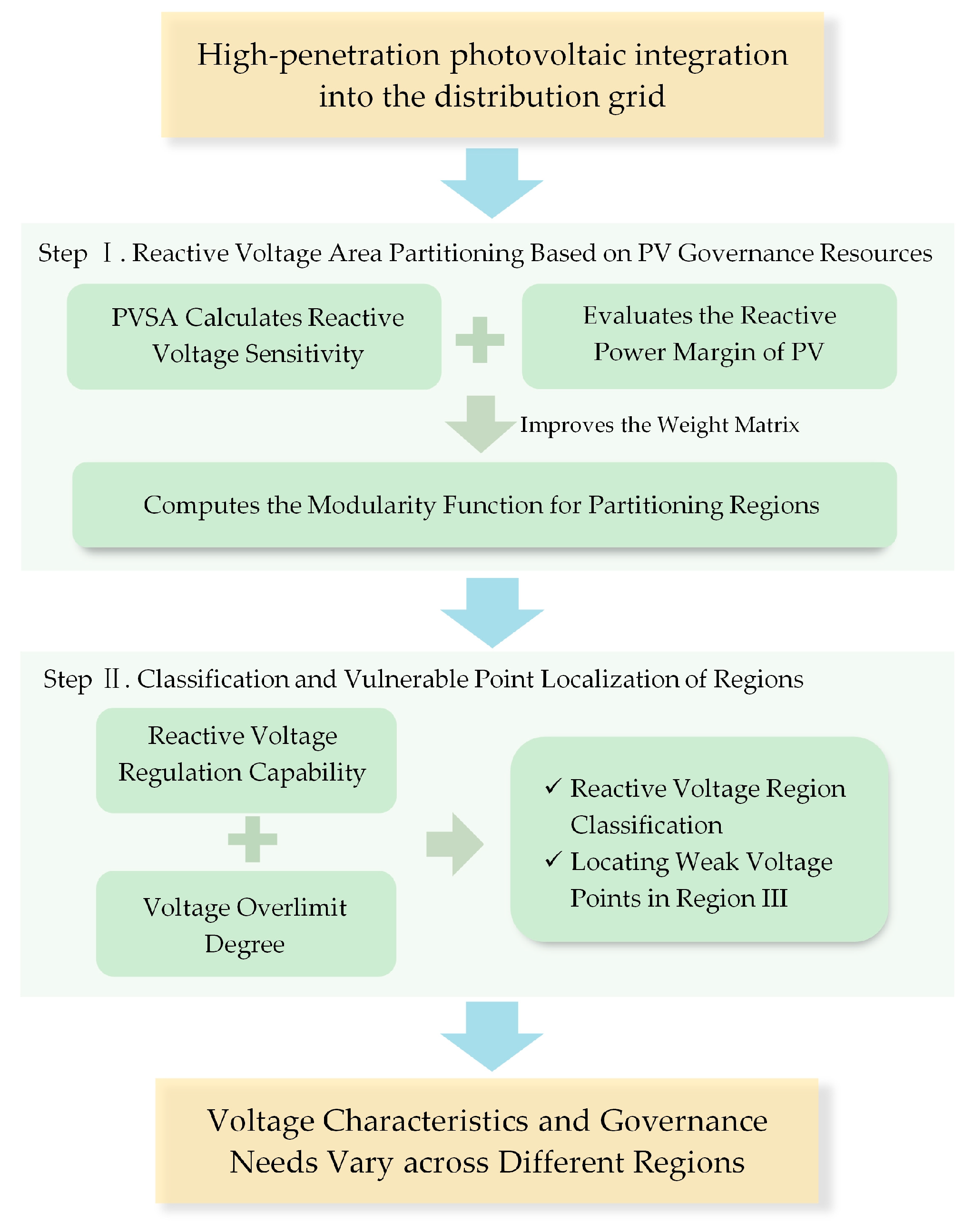
Propose a voltage partitioning strategy for distribution networks that considers PV reactive power margin. By refining the modularity function to partition voltage regions, this strategy classifies regions based on their internal regulation capabilities and identifies voltage weak points, allowing for precise management of voltage areas.

(iii)

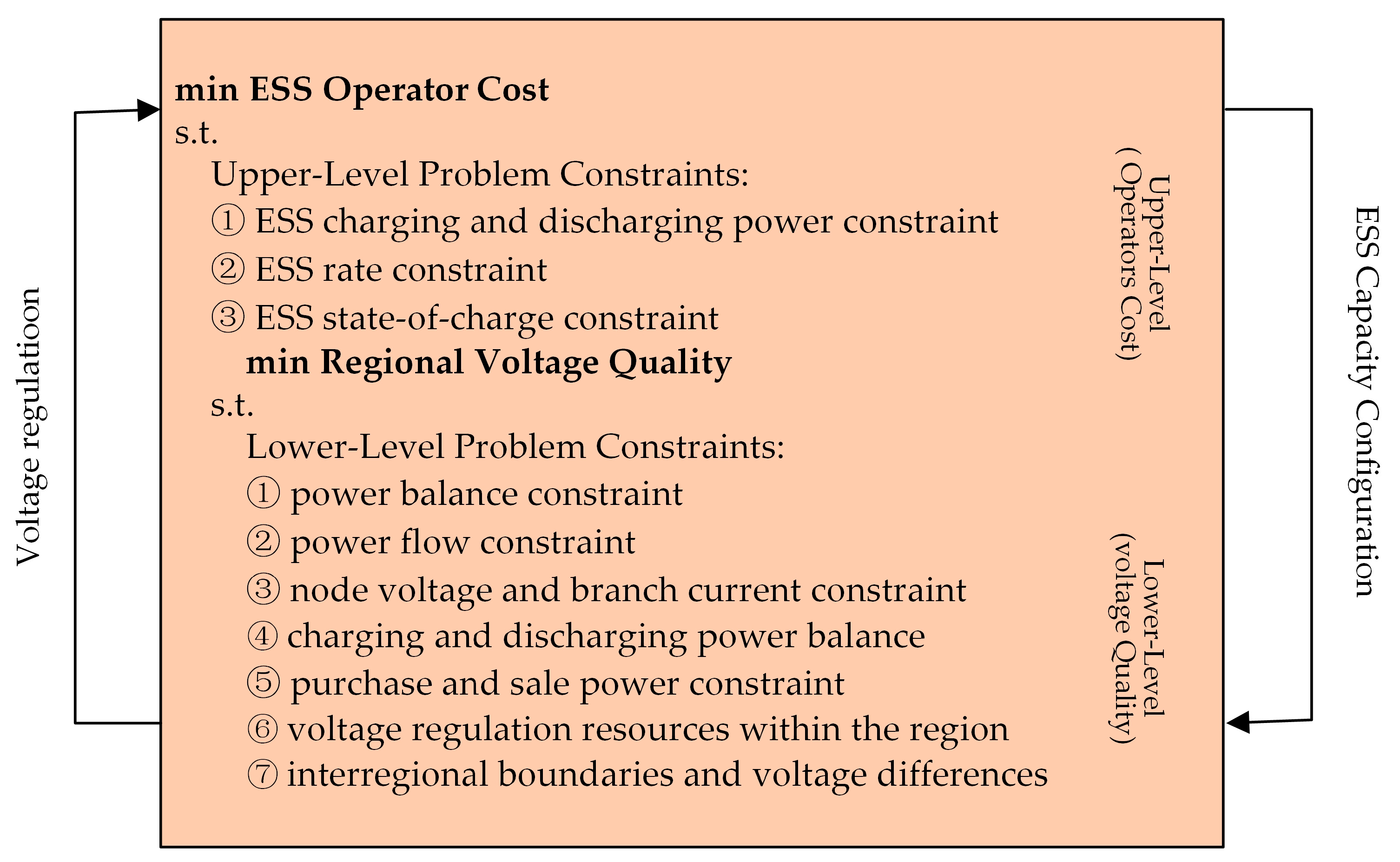
Establish a dual-layer optimization configuration model for ESSs that accounts for voltage regulation. The upper-layer model focuses on planning configurations that minimize operational costs for an ESS, while the lower-layer model optimizes scheduling to achieve the best regional voltage quality. This model defines voltage regulation constraints based on regional division, enabling optimization from regional to global levels.

(iv)

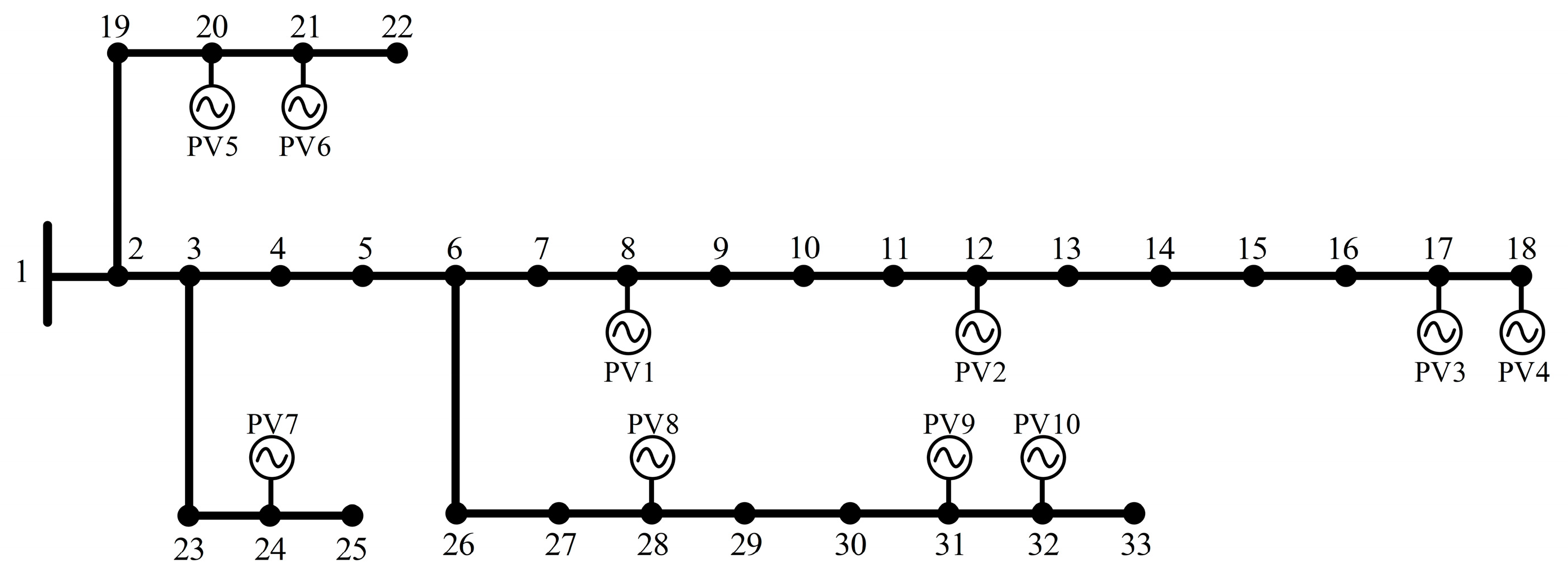
Compare the economic and voltage regulation effects across four scenarios to demonstrate the effectiveness and advantages of the proposed control strategy within the IEEE 33-node distribution network. This analysis also evaluates the rationality of voltage region division and the photovoltaic energy consumption rate.

2. Voltage Hierarchical Control of Distribution Networks Considering Photovoltaic and ESS Participation

2.1. Impact of Photovoltaic and ESS Integration on Distribution Network Voltage

The integration of distributed photovoltaics into the distribution network alters the magnitude and direction of the power flow within the existing system. Consequently, the voltage distribution along the feeder undergoes a transition from its original monotonic decrease to potentially exhibiting local maximum values, thereby resulting in voltage excursions at certain connection points [25]. By using the sustainable margin of grid-connected inverters to generate inductive reactive power or by utilizing the ESS to absorb active power, the voltage at the grid connection point can be reduced. Figure 1 illustrates a schematic representation of a distribution network feeder interconnected with PV and ESSs.

It is evident that photovoltaic grid-connected power generation elevates the voltage level at the connection point, whereas leveraging the controllable margin of the grid-connected inverter to produce inductive reactive power or employing an ESS to absorb active power can mitigate the voltage at the connection point.

Upon the integration of PV and ESSs into the distribution network, the voltage at the grid connection point is expressed as follows:

$$U_{\mathrm{n}}=U_{\mathrm{m}}-{\displaystyle \frac{({\displaystyle \sum _{i=n}^k}{P}_{\mathrm{i},\mathrm{L}}-P_{\mathrm{PV}}-P_{\mathrm{ESS}})R+({\displaystyle \sum _{i=n}^k}{Q}_{\mathrm{i},\mathrm{L}}-Q_{\mathrm{PV}})X}{U_{\mathrm{m}}}}$$

(1)

where Q_PV represents the reactive power emitted by distributed photovoltaics, with positive values denoting inductance and negative values denoting capacitance. Similarly, P_ESS signifies the charging and discharging power of the ESS, where positive values indicate discharging and negative values denote charging.

2.2. Assessment of Voltage Regulation Resources for Distributed Photovoltaics

The implementation of reactive power control via photovoltaic grid-connected inverters contributes to the amelioration of voltage deviations within distribution networks. By decoupling active and reactive currents through the manipulation of both the voltage outer loop and the current inner loop, these inverters enable active power output to the grid while simultaneously regulating reactive power compensation [26]. Herein, S denotes the total capacity of the photovoltaic grid-connected inverter, P represents the active power of grid-connected power generation, and Q denotes the reactive power for voltage improvement. Additionally, constant power factor control is employed, with further elaboration provided below:

$$\left\{\begin{array}{l}{P}^2+Q^2\le {(1.1S)}^2\hfill \\ \cos \phi =\cos \arctan (Q/P)\hfill \end{array}\right.$$

(2)

where the total photovoltaic output is constrained to no more than 1.1 times the inverter capacity and $\cos \phi$ denotes the power factor. This formulation takes into consideration both the reactive power margin and the capacity of the photovoltaic inverter itself, thereby promoting the rational alignment of its reactive power margin with reactive power tasks.

The temporal characteristics of PV power generation are seasonally dependent, with minimal variation in light intensity within the same season and significant differences across different seasons. By simulating the PV power generation model, the output of the corresponding time series is obtained. Subsequently, the reactive power management resources that can improve voltage quality in the distribution network are evaluated according to Equation (2).

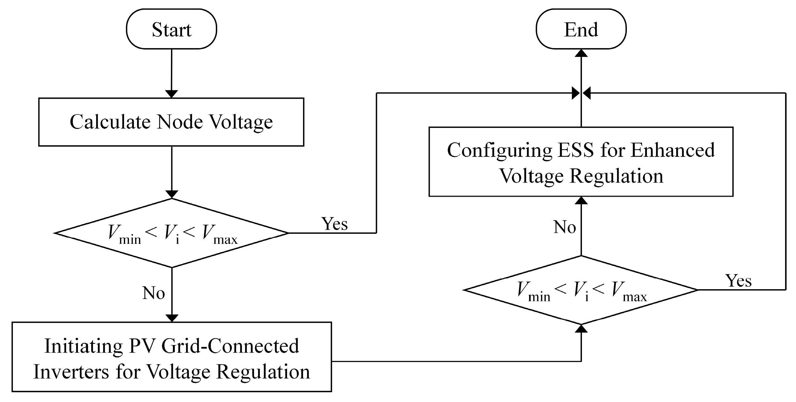
2.3. Hierarchical Voltage Control Based on Active and Reactive Power Coordination

To fully utilize the existing voltage regulation resources in the distribution network, we first assess whether the reactive power adjustable margin of PV can meet the voltage regulation requirements. If it is insufficient to maintain the node voltage of the distribution network within the national standard range, ESS active power is configured and utilized to participate in active voltage regulation. Accordingly, this article proposes a voltage layered control method for distribution networks that incorporates the participation of both PV and ESSs, as illustrated in Figure 2.

It is crucial to understand the voltage characteristics and regulation requirements of different regions to effectively configure ESSs for active participation in voltage management. Achieving energy balance within each region of the distribution network is facilitated through the collaborative strategy of photovoltaic storage. The voltage regional autonomy capability refers to the voltage regulation capacity of photovoltaic storage within each region of the distribution network.

3. Voltage Zoning Strategy for Distribution Networks Considering Photovoltaic Management Resources

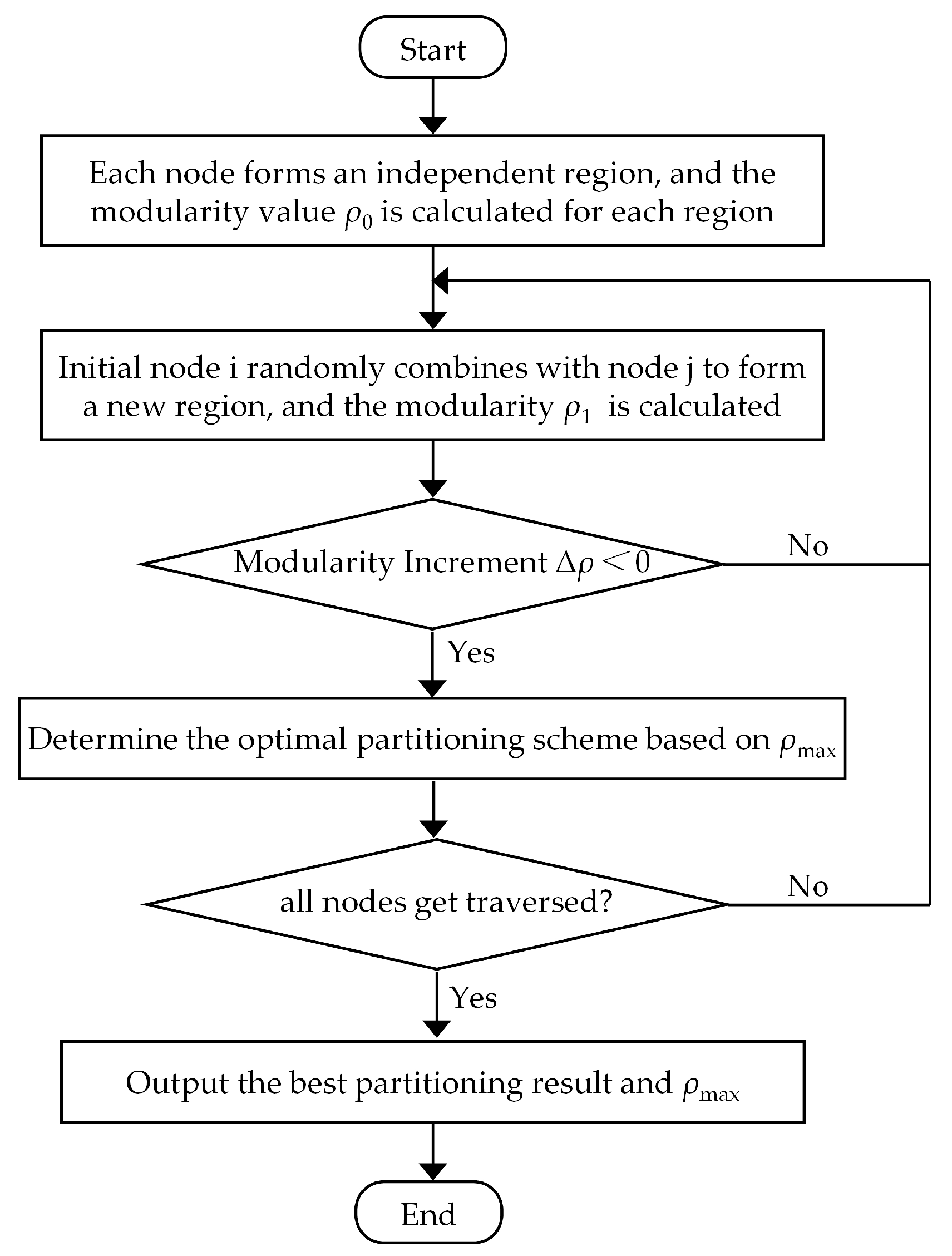
3.1. Modular Function Based on Photovoltaic Reactive Power Margin

Calculating the reactive voltage sensitivity of the distribution network using PVSA [27]. Figure 3 depicts a schematic diagram illustrating a typical radial network topology. Assuming a power disturbance ΔS_a at node a, the approximate reactive voltage sensitivity from node o to node a can be expressed as follows [28,29]:

$$S_{\mathrm{VQ},\mathrm{oa}}={\displaystyle \frac{\partial V_o}{\partial Q_a}}={\left|{\displaystyle \frac{\mathsf{\Delta }{S}_{\mathrm{a}}{Z}_{oa}}{V_a^{*}}}\right|}_{\mathsf{\Delta }{S}_{\mathrm{a}}=i}=\left|{\displaystyle \frac{\mathrm{i}{Z}_{oa}}{V_a^{*}}}\right|$$

(3)

where $V_a^{\ast }$ denotes the conjugate complex number of the voltage at the disturbed node a, and Z_oa represents the impedance of the shared tie line connecting the disturbed node a with the network node, as well as the observation node o with the network node.

The partition strategy aims to optimize overall voltage quality by incorporating the reactive power management resources of PV within the region. This approach involves constructing a modular function that accounts for reactive voltage sensitivity and the voltage support capability of PV, as detailed below:

$${\rho }_{\mathrm{VQ}}={\displaystyle \frac{1}{2m}}{\displaystyle \sum _i{\displaystyle \sum _j(A_{\mathrm{VQ},\mathrm{ij}}-\frac{k_i{k}_j}{2m})}}\delta (i,j)$$

(4)

$$A_{\mathrm{VQ},\mathrm{ij}}={\eta }_{\mathrm{VQ},\mathrm{ij}}+{\alpha }_{\mathrm{VQ},\mathrm{ij}}$$

(5)

where A_VQ,ij denotes the improved weight matrix between node i and node j, and A_ij represents the edge weight between node i and node j. When nodes are directly connected, A_ij = 1, and when they are not, A_ij = 0. The parameter $m=\left({\displaystyle {\sum }_i{\displaystyle {\sum }_j{A}_{\mathrm{ij}}}}\right)/2$ signifies half the sum of weights of all edges within the area while $k_i={\displaystyle {\sum }_i{A}_{\mathrm{ij}}}$ represents the sum of weights of all edges connected to node i. If nodes i and j are within the same area, $\delta (i,j)$ equals 1; otherwise, it equals 0. ${\eta }_{\mathrm{VQ},\mathrm{ij}}$ represents the reactive voltage sensitivity matrix, while ${\alpha }_{\mathrm{VQ},\mathrm{ij}}$ denotes the voltage support parameter.

The reactive voltage sensitivity matrix accurately characterizes the degree of reactive coupling between different nodes, comprehensively illustrating the bidirectional relationships and interconnections between nodes, as shown in Equation (6).

$${\eta }_{\mathrm{VQ},\mathrm{ij}}={\displaystyle \frac{S_{\mathrm{VQ},\mathrm{ij}}+S_{\mathrm{VQ},\mathrm{ji}}}{2}}$$

(6)

where S_VQ,ij denotes the reactive voltage sensitivity factor from node i to node j.

The voltage support capability of PV nodes varies with different reactive power margins, impacting not only the reactive power balance within the region but also the outcomes of regional division. Adjusting the reactive power of node i can enhance the voltage support capability of node j, as shown in Equation (7).

$${\alpha }_{\mathrm{VQ},\mathrm{ij}}={\displaystyle \frac{S_{\mathrm{VQ},\mathrm{ij}}}{S_{\mathrm{VQ},\mathrm{jj}}}}\times Q_{\mathrm{VQ},\mathrm{i}}$$

(7)

where Q_VQ,i represents the adjustable reactive power margin of the grid-connected inverter at node i.

By comprehensively considering reactive voltage sensitivity and photovoltaic inverter reactive power margin, the physical attributes of the distribution network can be effectively reflected. Through precise evaluation of node correlations and optimized deployment of photovoltaic distribution, the most suitable approach for voltage partitioning can be determined based on local conditions. This allows for the maximization of voltage improvement effects within the constraints of available governance resources.

3.2. Classification and Weak Point Localization of Distribution Network Regions

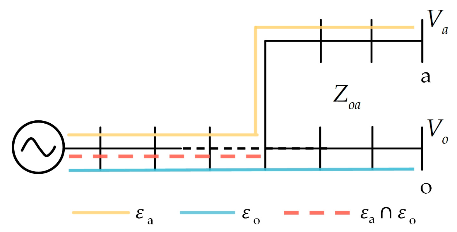
3.2.1. Division of Distribution Network Reactive Power Voltage Regions

Based on Figure 4, the calculation of reactive power and voltage modularity can achieve an optimized division of PV reactive power control areas in the distribution network. This article proposes a reactive power voltage regulation capability index for voltage region classification, defined as the ability of the adjustable reactive power from photovoltaic resources within the region to regulate node voltage quality. Specifically,

$${\phi }_{{\mathrm{Q},\mathrm{R}}_{\mathrm{k}}}=\left\{\begin{array}{cc}1& Q_{\mathrm{Sub}}⩾Q_{\mathrm{Need}},Q_{\mathrm{Need}}=0\\ \left|{\displaystyle \frac{Q_{\mathrm{Sub}}}{Q_{\mathrm{Need}}}}\right|& Q_{\mathrm{Sub}}<Q_{\mathrm{Need}}\end{array}\right.$$

(8)

$$Q_{\mathrm{Need}}={\displaystyle \sum _{i\in R_k}\frac{\mathsf{\Delta }{V}_{\mathrm{i}}}{S_{\mathrm{VQ},\mathrm{ii}}}}$$

(9)

where R_k represents the k-th region in the set R, with k ranging from 1 to the total number of regions; ${\phi }_{Q,R_{\mathrm{k}}}$ is the reactive power sensitivity in region R_k. When the reactive power compensation margin that photovoltaics can provide is greater than the required reactive power, or when photovoltaic compensation is not needed, ${\phi }_{Q,R_{\mathrm{k}}}=1$; otherwise, ${\phi }_{Q,R_{\mathrm{k}}}<1$. Q_Sub is the reactive power compensation margin that distributed photovoltaics can provide in region R_k, Q_Need is the minimum value of the required reactive power, ΔV_i is the voltage increment of node I, and S_VQ,ii is the reactive voltage sensitivity of photovoltaic node i in region R_k.

During voltage fluctuations, the voltage areas within the distribution network can be categorized into three distinct classes: Region I, where node voltages remain within normal limits and possess adequate adjustment capabilities; Region II, characterized by voltage exceedance at select nodes yet still possessing sufficient adjustment capabilities within the area; and Region III, where the majority of node voltages surpass the limits, indicative of insufficient regional adjustment capabilities. Correspondingly, Class I and II areas implement first-layer voltage control, while Class III areas use double-layer voltage control.

In accordance with the hierarchical control of distribution network voltage, consideration of the location and capacity of the ESS is warranted within Region III. This approach aims to optimize the utilization of the ESS to mitigate the impact of photovoltaic power fluctuations on the distribution network, thereby enhancing coordination between photovoltaic output reactive power and ESS active power consumption to augment the voltage autonomy of the power grid.

3.2.2. Localization and Evaluation of Voltage Weak Points

The categorization of voltage regions and identification of their vulnerable points serve to elucidate the voltage characteristics and regulatory requisites across diverse regions. This insight facilitates the adoption of tailored strategies aimed at enhancing the overall voltage profile of the distribution network. Voltage weak points denote particular nodes within the distribution network exhibiting the most significant voltage deviations or fluctuations, potentially jeopardizing the network’s stability and compromising voltage quality. Thus, the selection of weak points considers both their voltage deviation and daily average voltage fluctuation. The formulation of the specific mathematical model is as follows:

$$\begin{array}{c}\max \left\{f_1,f_2\right\}\\ \left\{\begin{array}{c}{f}_1={\displaystyle \sum _{d=1}^D{\displaystyle \sum _{t=1}^{N_T}{\displaystyle \sum _{i=1}^N{T}_{\mathrm{d}}\mathsf{\Delta }t\left|U_{\mathrm{d},\mathrm{t},\mathrm{i}}^2(t)-1\right|}}}\\ f_2={\displaystyle \sum _{i=1}^N\sqrt{\frac{{\displaystyle \sum _{t=1}^{N_{\mathrm{T}}}}{\left(U_{\mathrm{d},\mathrm{t},\mathrm{i}}(t)-{\overline{U}}_{\mathrm{i}}\right)}^2}{N_{\mathrm{T}}}}}\end{array}\right.\end{array}$$

(10)

where U_d,t,i(t) denotes the per unit voltage value of node i during typical daily period t, and ${\overline{U}}_i$ represents the daily average voltage of node i.

The voltage improvement potential, derived from the adjustable active and reactive power capacities of photovoltaic and ESS resources within a given region, serves as a pivotal indicator of observability for voltage weak points. Specifically,

$${\phi }_{\mathrm{V}}^{\mathrm{i},\mathrm{t}}=\left\{\begin{array}{ll}1\hfill & \mathsf{\Delta }{V}_{\mathrm{i}}<\mathsf{\Delta }{V}_{\max }^{\mathrm{i}}\\ \mathsf{\Delta }{V}_{\max }^{\mathrm{i}}/\mathsf{\Delta }{V}_{\mathrm{i}}\hfill & \mathsf{\Delta }{V}_{\mathrm{i}}\ge \mathsf{\Delta }{V}_{\max }^{\mathrm{i}}\end{array}\right.$$

(11)

$$\left\{\begin{array}{l}\mathsf{\Delta }{V}_{\max }^{\mathrm{i}}={\displaystyle \sum \left(S_{\mathrm{VP},\mathrm{ij}}\sum \mathsf{\Delta }{P}_{\max }^{\mathrm{j},\mathrm{t}}+S_{\mathrm{VQ},\mathrm{ij}}\sum \mathsf{\Delta }{Q}_{\max }^{\mathrm{j},\mathrm{t}}\right)}\\ \mathsf{\Delta }{P}_{\max }^{\mathrm{j},\mathrm{t}}={\displaystyle \sum \left(\mathsf{\Delta }{P}_{\mathrm{pv},\mathrm{m}}^{\mathrm{j},\mathrm{t}}+P_{\mathrm{ess},\mathrm{m}}^{\mathrm{j},\mathrm{t}}\right)}\\ \mathsf{\Delta }{Q}_{\max }^{\mathrm{j},\mathrm{t}}={\displaystyle \sum \left(Q_{\mathrm{pv},\mathrm{m}}^{\mathrm{j},\mathrm{t}}+Q_{\mathrm{ess},\mathrm{m}}^{\mathrm{j},\mathrm{t}}\right)}\end{array}\right.$$

(12)

where ${\phi }_{\mathrm{V}}^{\mathrm{i},\mathrm{t}}$ represents the voltage enhancement potential index of weak point i, $\mathsf{\Delta }{V}_{\mathrm{i}}$ denotes the voltage deviation magnitude of weak point i within the region, and $\mathsf{\Delta }{V}_{\max }^{\mathrm{i}}$ designates the maximum voltage adjustment extent of weak point i when accounting for the active–reactive power margin within the region. All these variables are directional indicators.

In conclusion, the distribution network voltage zoning strategy, taking into account photovoltaic governance resources, is illustrated in Figure 5.

4. Considering Regional Voltage Regulation in Energy Storage System Dual-Layer Optimization Configuration Model

Based on the division of PV reactive power margins into voltage regions, the first layer of reactive power voltage regulation has been achieved. Considering the hierarchical control of PV storage, this article adopts a shared economy ESS service model. This model involves selecting sites, investing in, and constructing ESS facilities within the distribution network to provide charging and discharging services. These services charge fees to users, meeting the voltage regulation needs of the distribution network while ensuring the economic feasibility of ESS investment and operation.

This article establishes a dual-layer optimization configuration model. The upper-layer configuration model aims to minimize the annual comprehensive operating cost of the ESS by optimizing the location and capacity of the storage facilities. The lower-level scheduling model focuses on optimizing the charging and discharging behavior of the ESS to improve regional voltage quality. By configuring the ESS, the distribution network’s ability to absorb new energy can be enhanced from a global perspective, thereby reducing PV waste. Figure 6 is a schematic diagram of the dual-layer optimization configuration model.

4.1. Upper-Layer Energy Storage System Planning Model

The upper-level model is tasked with resolving the optimal annual comprehensive operating cost of the ESS throughout the planning horizon. The decision variables encompass the capacity configuration and maximum charge and discharge power of the ESS.

4.1.1. Objective Function of Upper-Layer Model

The primary optimization objective at the upper level is to minimize the annual comprehensive operating cost of the ESS, comprising three main components: the average daily investment and maintenance cost of the ESS, typical daily income, and associated service fees, as depicted in the subsequent formula:

$$\min C={\displaystyle \sum _{d=1}^D[T_{\mathrm{d}}(C_{\mathrm{inv},\mathrm{d}}+C_{\mathrm{ess},\mathrm{d}}-C_{\mathrm{serve},\mathrm{d}})]}$$

(13)

where d represents the number of typical days, T_d denotes the number of days corresponding to the d-th typical day, C_inv,d stands for the average daily investment and maintenance cost of the ESS, C_ess,d represents the electricity purchase and sale of the ESS on each typical day, and C_serve,d signifies the ESS service fee per typical day.

(1)

The mean daily expenditure for investment and maintenance of the ESS [30] is

$$C_{\mathrm{inv},\mathrm{d}}={\displaystyle \frac{{\eta }_{\mathrm{P}}{P}_{\mathrm{ess}}^{\max }+{\eta }_{\mathrm{S}}{E}_{\mathrm{ess}}^{\max }}{T_{\mathrm{s}}}}+M_{\mathrm{ess}}$$

(14)

where ${\eta }_{\mathrm{P}}$ and ${\eta }_{\mathrm{S}}$ represent the power cost and capacity cost of the ESS respectively, measured in yuan/kW and yuan/kWh respectively; $P_{\mathrm{ess}}^{\max }$ and $E_{\mathrm{ess}}^{\max }$ denote the maximum charge and discharge power and maximum capacity of the ESS, respectively; T_s signifies the expected number of days of use of the ESS; and M_ess denotes the daily maintenance cost.

(2)

The electricity purchase and sale revenue of the ESS for each typical day is

$$C_{\mathrm{ess},\mathrm{r},\mathrm{d}}={\displaystyle \sum _{i=1}^N{\displaystyle \sum _{t=1}^{N_{\mathrm{T}}}\left[\left(\delta (t)\cdot P_{\mathrm{ess},\mathrm{s},\mathrm{d},\mathrm{i}}(t)-\lambda (t)\cdot P_{\mathrm{ess},\mathrm{b},\mathrm{d},\mathrm{i}}(t)\right)\cdot \mathsf{\Delta }t\right]}}$$

(15)

where N represents the number of distribution networks in Region III and N_T corresponds to the number of dispatch cycle periods. $\delta (t)$ denotes the electricity price of the distribution network selling electricity to the ESS in period t, while P_ess,s,d,i(t) indicates the electricity price of each typical day, reflecting the i-th region’s sale of electricity to the ESS during period t. Additionally, λ(t) represents the electricity price for the distribution network to purchase electricity from the ESS during period t. Moreover, P_ess,b,d,i(t) stands for the i-th period of each typical day region t purchases power from the ESS, with t symbolizing the dispatch period.

(3)

The service fee collected by the ESS from the distribution network on each typical day is

$$C_{\mathrm{serve},\mathrm{d}}={\displaystyle \sum _{i=1}^N{\displaystyle \sum _{t=1}^{N_{\mathrm{T}}}\left\{\theta (t)\cdot \left[P_{\mathrm{ess},\mathrm{b},\mathrm{d},\mathrm{i}}(t)+P_{\mathrm{ess},\mathrm{s},\mathrm{d},\mathrm{i}}(t)\right]\cdot \mathsf{\Delta }t\right\}}}$$

(16)

where $\theta (t)$ represents the unit price of service fees paid by the distribution network to the ESS during period t, measured in yuan/(kWh). Users pay service fees to energy storage operators to purchase ESSs to meet their charging and discharging needs, eliminating the investment and installation maintenance costs of ESSs; users pay service fees with an annual settlement cycle, and the energy storage control center monitors user usage. The ESS stores the total power Q₁, releases the total power Q₂, and calculates the service fee required by the user according to the equation (Q₁ + Q₂).

4.1.2. Constraints of Upper-Layer Model

(1)

Constraints on the charging and discharging power of ESSs are imposed. These constraints are subject to economic costs, node voltage limitations, and branch current restrictions. They include limitations on the upper bounds of electric power capacity bought and sold by each ESS, ensuring that its energy capacity exceeds its power capacity.

$$\left\{\begin{array}{l}0\le P_{\mathrm{ess},\mathrm{abs}}(t)\le U_{\mathrm{abs}}(t)P_{\mathrm{ess}}^{\max }\hfill \\ 0\le P_{\mathrm{ess},\mathrm{relea}}(t)\le U_{\mathrm{relea}}(t)P_{\mathrm{ess}}^{\max }\hfill \\ U_{\mathrm{abs}}(t)+U_{\mathrm{relea}}(t)\le 1\hfill \\ U_{\mathrm{abs}}(t)\in \left\{0,1\right\},U_{\mathrm{relea}}(t)\in \left\{0,1\right\}\hfill \end{array}\right.$$

(17)

where P_ess,abs(t) and P_ess,relea(t) represent the charging and discharging power of the ESS, respectively; U_abs(t) and U_relea(t) denote the charging and discharging status indicators of the ESS, which are binary variables ranging from 0 to 1.

(2)

ESS rate constraints are governed by a direct proportionality between the system’s capacity and its rated power [25].

$$E_{\mathrm{ess}}^{\max }=\beta P_{\mathrm{ess}}^{\max }$$

(18)

where β represents the ESS energy rating.

(3)

ESS state-of-charge constraints entail maintaining the storage energy operating range within 10% to 90%. The initial stored energy is set at 20%, and a 10% difference in the state of charge between the beginning and the end is upheld to ensure the continuity and reliability of its long-term operation.

$$\left\{\begin{array}{l}{E}_{\mathrm{ess}}(t)=E_{\mathrm{ess}}(t-1)+[{\eta }^{\mathrm{abs}}{P}_{\mathrm{ess},\mathrm{abs}}(t)-{\displaystyle \frac{1}{{\eta }^{\mathrm{relea}}}}{P}_{\mathrm{ess},\mathrm{relea}}(t)]\mathsf{\Delta }t\hfill \\ E_{\mathrm{ess}}(0)=20\%E_{\mathrm{ess}}^{\max }\hfill \\ 10\%E_{\mathrm{ess}}^{\max }\le E_{\mathrm{ess}}(t)\le 90\%E_{\mathrm{ess}}^{\max }\hfill \\ 10\%\le \left|E_{\mathrm{ess}}(0)-E_{\mathrm{ess}}(24)\right|\le 10\%\end{array}\right.$$

(19)

where E_ess(t) represents the energy stored in the ESS at time t, and ${\eta }^{\mathrm{abs}}$ and ${\eta }^{\mathrm{relea}}$ denote the charging efficiency and discharge efficiency of the energy storage device, respectively. Additionally, E_ess(0) and E_ess(24) signify the stored energy of the ESS at the beginning and end of the operational period, respectively.

4.2. Lower-Layer Regional Voltage Optimization Model

The lower layer formulates an optimal dispatch model aimed at enhancing voltage quality within the distribution network region, achieved through active adjustments of the ESS. The operation of ESSs dynamically adjusts grid voltage and power to align with peak periods of photovoltaic power generation and low periods of electricity demand.

4.2.1. Objective Function of Lower-Layer Model

The lower-level objective function aims to optimize the regional voltage quality of the distribution network through the engagement of PV and ESS in regulation. Evaluation criteria include voltage deviation and daily average voltage fluctuations. The specifics are outlined as follows:

$$\min F=\min \left\{f_{1,R_{\mathrm{k}}},f_{2,R_{\mathrm{k}}}\right\}$$

(20)

4.2.2. Constraints of Lower-Layer Model

(1)

Power balance constraint

$$\left\{\begin{array}{l}\begin{array}{l}{\displaystyle \sum _{i\in a_{\mathrm{k}}(j)}(P_{\mathrm{d},\mathrm{ij}}(t)-l_{\mathrm{d},\mathrm{ij}}{r}_{\mathrm{ij}})}+P_{\mathrm{grid},\mathrm{d},\mathrm{j}}(t)+P_{\mathrm{pv},\mathrm{d},\mathrm{j}}(t)+\\ P_{\mathrm{ess},\mathrm{relea},\mathrm{d}}(t)-P_{\mathrm{ess},\mathrm{abs},\mathrm{d}}(t)-P_{\mathrm{load},\mathrm{d},\mathrm{j}}(t)={\displaystyle \sum _{i\in c_k(j)}{P}_{\mathrm{d},\mathrm{jm}}(t):{\lambda }_{1,\mathrm{t},\mathrm{d}}}\end{array}\hfill \\ \begin{array}{l}{\displaystyle \sum _{i\in a_{\mathrm{k}}(j)}(Q_{\mathrm{d},\mathrm{ij}}(t)-l_{\mathrm{d},\mathrm{ij}}{x}_{\mathrm{ij}})}+Q_{\mathrm{grid},\mathrm{d},\mathrm{j}}(t)+Q_{\mathrm{pv},\mathrm{d},\mathrm{j}}(t)+\\ Q_{\mathrm{ess},\mathrm{relea},\mathrm{d}}(t)-Q_{\mathrm{ess},\mathrm{abs},\mathrm{d}}(t)-Q_{\mathrm{load},\mathrm{d},\mathrm{j}}(t)={\displaystyle \sum _{i\in c_{\mathrm{k}}(j)}{Q}_{\mathrm{d},\mathrm{jm}}(t):{\lambda }_{2,\mathrm{t},\mathrm{d}}}\end{array}\hfill \end{array}\right.$$

(21)

where a_k(j) represents the set of all first endpoints of branches with j as one endpoint in distribution network area k, and c_k(j) denotes the set of all endpoints of branches with j as the first endpoint in distribution network area k. P_d,ij(t), P_d,jm(t), Q_d,ij(t), and Q_d,jm(t) signify the active and reactive powers at the starting and ending points of branches ij and jm in period t on typical day d, respectively. l_d,ij represents the square of the current amplitude of branch ij, while r_ij and x_ij denote the resistance and reactance of branch ij, respectively. P_grid,d,j(t) and Q_grid,d,j(t) signify the active and reactive powers injected into node j by the grid during period t on typical day d. Similarly, P_pv,d,j(t) and Q_pv,d,j(t) represent the active and reactive powers injected into node j by the photovoltaic system, while P_load,d,j(t) and Q_load,d,j(t) indicate the active and reactive powers of the load at node j, respectively.

(2)

Power flow constraint

$${‖{\left[\begin{array}{ccc}2P_{\mathrm{d},\mathrm{ij}}& 2P_{\mathrm{d},\mathrm{ij}}& l_{\mathrm{d},\mathrm{ij}}-u_{\mathrm{d},\mathrm{i}}\end{array}\right]}^T‖}_2\le l_{\mathrm{d},\mathrm{ij}}+u_{\mathrm{d},\mathrm{i}}$$

(22)

where $u_{\mathrm{d},\mathrm{i}}(t)=U_{\mathrm{d},\mathrm{i}}^2(t)$ and $l_{\mathrm{d},\mathrm{ij}}(t)=I_{\mathrm{d},\mathrm{ij}}^2(t)$ are relaxed.

(3)

Node voltage and branch current constraints

$$u_{\mathrm{d},\mathrm{j}}(t)=u_{\mathrm{d},\mathrm{i}}(t)-2(r_{\mathrm{ij}}{P}_{\mathrm{d},\mathrm{ij}}(t)+x_{\mathrm{ij}}{Q}_{\mathrm{d},\mathrm{ij}}(t))+(r_{\mathrm{ij}}^2+x_{\mathrm{ij}}^2)l_{\mathrm{d},\mathrm{ij}}(t):{\lambda }_{3,\mathrm{t},\mathrm{d}}$$

(23)

$${(U_{\mathrm{d},\mathrm{i}}^{\min })}^2\le u_{\mathrm{d},\mathrm{i}}(t)\le {(U_{\mathrm{d},\mathrm{i}}^{\max })}^2:{\mu }_{1,\mathrm{t},\mathrm{d}}^{\min },{\mu }_{1,\mathrm{t},\mathrm{d}}^{\max }$$

(24)

$$0\le l_{\mathrm{d},\mathrm{ij}}(t)\le {(I_{\mathrm{d},\mathrm{ij}}^{\max })}^2:{\mu }_{2,\mathrm{t},\mathrm{d}}^{\min },{\mu }_{2,\mathrm{t},\mathrm{d}}^{\max }$$

(25)

where $U_{\mathrm{d},\mathrm{i}}^{\max }$ and $U_{\mathrm{d},\mathrm{i}}^{\min }$ represent the maximum and minimum voltage amplitude limits of node i during period t on typical day d, respectively, and $I_{\mathrm{d},\mathrm{ij}}^{\max }$ denotes the safety current of branch ij during period t on typical day d.

(4)

ESS charging and discharging power balance constraint

$$P_{\mathrm{ess},\mathrm{b},\mathrm{w}}(t)-P_{\mathrm{ess},\mathrm{s},\mathrm{w}}(t)=P_{\mathrm{ess},\mathrm{realea}}(t)-P_{\mathrm{ess},\mathrm{abs}}(t):{\lambda }_{4,\mathrm{t},\mathrm{d}}$$

(26)

(5)

Purchase and sale power constraints between the distribution network and ESSs

$$\left\{\begin{array}{l}0\le P_{\mathrm{ess},\mathrm{s},\mathrm{d}}(t)\le P_{\mathrm{ess},\mathrm{mg}}^{\max }:{\mu }_{3,\mathrm{t},\mathrm{d}}^{\min },{\mu }_{3,\mathrm{t},\mathrm{d}}^{\max }\hfill \\ 0\le P_{\mathrm{ess},\mathrm{b},\mathrm{d}}(t)\le P_{\mathrm{ess},\mathrm{mg}}^{\max }:{\mu }_{4,\mathrm{t},\mathrm{d}}^{\min },{\mu }_{4,\mathrm{t},\mathrm{d}}^{\max }\hfill \\ U_{\mathrm{buy},\mathrm{d}}(t)+U_{\mathrm{sale},\mathrm{d}}(t)\le 1:{\mu }_{5,\mathrm{t},\mathrm{d}}^{\min },{\mu }_{5,\mathrm{t},\mathrm{d}}^{\max }\hfill \end{array}\right.$$

(27)

where $P_{\mathrm{ess},\mathrm{mg}}^{\max }$ represents the maximum interaction power between the distribution network and the ESS. U_buy,d(t) and U_sale,d(t) denote the power purchase and sales status between the ESS and each typical day, respectively.

(6)

Constraints on voltage regulation resources within the region

$$\left\{\begin{array}{l}0<{\phi }_{Q,R_{\mathrm{k}}}<1:{\mu }_{6,\mathrm{t},\mathrm{d}}^{\min },{\mu }_{6,\mathrm{t},\mathrm{d}}^{\max }\hfill \\ {\phi }_{\mathrm{V}}^{\mathrm{i},\mathrm{t}}=1:{\lambda }_{5,\mathrm{t},\mathrm{d}}\hfill \end{array}\right.$$

(28)

where constraints are placed on the reactive power and voltage control capabilities of Region III, as well as on the voltage improvement potential of weak points.

(7)

Constraints on interregional voltage differences

$$\left|f_{1,R_{\mathrm{m}}}-f_{1,R_{\mathrm{n}}}\right|\le 0.04:{\mu }_{7,\mathrm{t},\mathrm{d}}^{\min },{\mu }_{7,\mathrm{t},\mathrm{d}}^{\max }$$

(29)

where the interval voltage difference is less than 0.04.

4.3. Solution of Dual-Layer Configuration Model

The aforementioned dual-layer model comprises integer variables, continuous variables, and nonlinear constraints in the upper layer, while the lower layer presents a mixed integer linear programming conundrum, posing a challenge for direct resolution (Figure 7). To attain the global optimum, this study endeavors to linearize the model, transforming it into a mixed integer linear programming issue and subsequently employing a solver to resolve it comprehensively.

This study constructs the Lagrangian function of the lower model, represented by Equation (30). Utilizing the KKT complementary relaxation condition, it is transformed into the constraint conditions of the upper-layer model. Subsequently, the Big-M method [31,32] is applied to linearize the nonlinear terms of the converted single-layer nonlinear model, thus forming a single-layer mixed integer linear programming problem. The transformed single-layer model is presented in (A1)–(A4) in Appendix A, where (A1) and (A2) denote the optimization objectives and constraints of the original upper-layer model.

$$\begin{array}{l}L=\min \{{\displaystyle \sum _{d=1}^D{\displaystyle \sum _{t=1}^{N_T}{\displaystyle \sum _{i=1}^N{T}_d\mathsf{\Delta }t\left|U_{\mathrm{d},\mathrm{t},\mathrm{i}}^2(t)-1\right|}}},{\displaystyle \sum _{i=1}^N\sqrt{\frac{{\displaystyle \sum _{t=1}^{N_T}}{\left(U_{\mathrm{d},\mathrm{t},\mathrm{i}}(t)-{\overline{U}}_i\right)}^2}{N_T}}}\}\\ +{\lambda }_{1,\mathrm{t},\mathrm{d}}[{\displaystyle \sum _{i\in a_k(j)}(P_{\mathrm{d},\mathrm{ij}}(t)-l_{\mathrm{d},\mathrm{ij}}{r}_{\mathrm{d},\mathrm{ij}})}+P_{\mathrm{grid},\mathrm{d},\mathrm{j}}(t)+P_{\mathrm{pv},\mathrm{d},\mathrm{j}}(t)+P_{\mathrm{ess},\mathrm{b},\mathrm{d}}(t)-P_{\mathrm{ess},\mathrm{s},\mathrm{d}}(t)-P_{\mathrm{load},\mathrm{d},\mathrm{j}}(t)-{\displaystyle \sum _{i\in c_k(j)}{P}_{\mathrm{d},\mathrm{jm}}(t)}]\\ +{\lambda }_{2,\mathrm{t},\mathrm{d}}[{\displaystyle \sum _{i\in a_k(j)}(Q_{\mathrm{d},\mathrm{ij}}(t)-l_{\mathrm{d},\mathrm{ij}}{x}_{\mathrm{d},\mathrm{ij}})}+Q_{\mathrm{grid},\mathrm{d},\mathrm{j}}(t)+Q_{\mathrm{pv},\mathrm{d},\mathrm{j}}(t)+Q_{\mathrm{ess},\mathrm{b},\mathrm{d}}(t)-Q_{\mathrm{ess},\mathrm{s},\mathrm{d}}(t)-Q_{\mathrm{load},\mathrm{d},\mathrm{j}}(t)-{\displaystyle \sum _{i\in c_k(j)}{Q}_{\mathrm{d},\mathrm{jm}}(t)}]\\ +{\lambda }_{3,\mathrm{t},\mathrm{d}}[u_{\mathrm{d},\mathrm{i}}(t)-u_{\mathrm{d},\mathrm{j}}(t)-2(r_{\mathrm{ij}}{P}_{\mathrm{d},\mathrm{ij}}(t)+x_{\mathrm{ij}}{Q}_{\mathrm{d},\mathrm{ij}}(t))+(r_{\mathrm{ij}}^2+x_{\mathrm{ij}}^2)l_{\mathrm{d},\mathrm{ij}}(t)]\\ +{\lambda }_{4,\mathrm{t},\mathrm{d}}[P_{\mathrm{ess},\mathrm{b},\mathrm{d}}(t)-P_{\mathrm{ess},\mathrm{s},\mathrm{d}}(t)-P_{\mathrm{ess},\mathrm{realea}}(t)+P_{\mathrm{ess},\mathrm{abs}}(t)]\\ +{\lambda }_{5,\mathrm{t},\mathrm{d}}[{\phi }_{\mathrm{V}}^{\mathrm{i},\mathrm{t}}-1]\\ +{\mu }_{1,\mathrm{t},\mathrm{d}}^{\min }[{(U_{\mathrm{d},\mathrm{i}}^{\min })}^2-u_{\mathrm{d},\mathrm{i}}(t))+{\mu }_{1,\mathrm{t},\mathrm{d}}^{\max }(u_{\mathrm{d},\mathrm{i}}(t)-{(U_{\mathrm{d},\mathrm{i}}^{\max })}^2]\\ -{\mu }_{2,\mathrm{t},\mathrm{d}}^{\min }{l}_{\mathrm{d},\mathrm{ij}}(t)+{\mu }_{2,\mathrm{t},\mathrm{d}}^{\max }[l_{\mathrm{d},\mathrm{ij}}(t)-{(I_{\mathrm{d},\mathrm{i}}^{\max })}^2]\\ -{\mu }_{3,\mathrm{t},\mathrm{d}}^{\min }{P}_{\mathrm{ess},\mathrm{s},\mathrm{d}}(t)+{\mu }_{3,\mathrm{t},\mathrm{d}}^{\max }[P_{\mathrm{ess},\mathrm{s},\mathrm{d}}(t)-P_{\mathrm{ess},\mathrm{mg}}^{\max }\cdot U_{\mathrm{sale},\mathrm{d}}(t)]\\ -{\mu }_{4,\mathrm{t},\mathrm{d}}^{\min }{P}_{\mathrm{ess},\mathrm{b},\mathrm{d}}(t)+{\mu }_{4,\mathrm{t},\mathrm{d}}^{\max }[P_{\mathrm{ess},\mathrm{b},\mathrm{d}}(t)-P_{\mathrm{ess},\mathrm{mg}}^{\max }\cdot U_{\mathrm{buy},\mathrm{d}}(t)]\\ +{\mu }_{5,\mathrm{t},\mathrm{d}}^{\max }[U_{\mathrm{buy},\mathrm{d}}(t)+U_{\mathrm{sale},\mathrm{d}}(t)-1]\\ -{\mu }_{6,\mathrm{t},\mathrm{d}}^{\min }{\phi }_{Q,R_{\mathrm{k}}}+{\mu }_{6,\mathrm{t},\mathrm{d}}^{\max }[{\phi }_{Q,R_{\mathrm{k}}}-1]\\ +{\mu }_{7,\mathrm{t},\mathrm{d}}^{\min }[f_{1,R_{\mathrm{n}}}-f_{1,R_{\mathrm{m}}}-0.04]+{\mu }_{7,\mathrm{t},\mathrm{d}}^{\max }[f_{1,R_{\mathrm{m}}}-f_{1,R_{\mathrm{n}}}-0.04]\end{array}$$

(30)

In the converted single-layer model, the nonlinear constraints within constraints (A2)–(A4) are treated using the Big-M method. This involves the introduction of several 0–1 variables to equivalently convert the original nonlinear constraints into mixed integer linear constraints. Equation (31) represents the linearization of the first constraint on the dual variable within the lower inequality constraints, with similar transformations applied to the remaining constraints.

$$\left\{\begin{array}{l}0\le {\mu }_{1,\mathrm{t},\mathrm{d}}^{\min }\le M{v}_{1,\mathrm{t},\mathrm{d}}^{\min }\hfill \\ 0\le u_{\mathrm{d},\mathrm{i}}(t)-{(U_{\mathrm{d},\mathrm{i}}^{\min })}^2\le M(1-v_{1,\mathrm{t},\mathrm{d}}^{\min })\hfill \end{array}\right.$$

(31)

where M represents a sufficiently large constant and $v_{1,\mathrm{t},\mathrm{d}}^{\min }$ is a binary variable.

5. Case Study

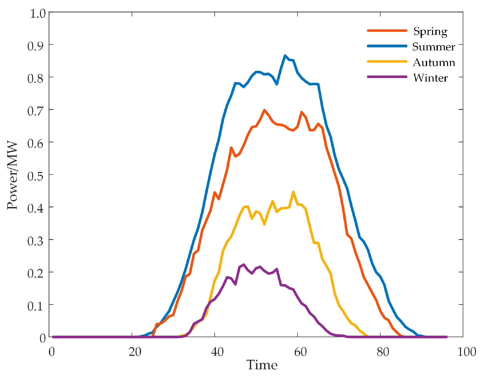
5.1. Case Introduction

To validate the efficacy and versatility of the proposed approach, a computational illustration is conducted utilizing an IEEE 33-node distribution network for analysis. The system’s nominal voltage is set at 11 kV, with a reference capacity of SB = 10 MVA, and the distribution network interfaces with the external power grid through node 1. Detailed system composition and parameters are documented in Ref. [33]. The model is solved using the GUROBI (11.0) solver implemented on the MATLAB platform. The computational hardware comprises an Intel(R) Core(TM) i7-12700H CPU clocked at 2.30 GHz, supported by 32 GB of memory.

Once the distributed power grid-connected points achieve uniform power quality standards, the permissible capacity for connection increases with higher node loads [34]. Consequently, this study designates nodes at the terminus of each branch or nodes with substantial load levels, specifically nodes 8, 12, 17, 18, 20, 21, 24, 28, 31, and 32, as photovoltaic access points. The distribution network topology is illustrated in Figure 8.

The photovoltaic output prediction is derived from comprehensive lighting and load operation data collected over the course of a year within a specific region, with a temporal resolution of 15 min. Depicted in Figure 9 is the photovoltaic output curve representative of a standard day. Each distributed photovoltaic grid-connected inverter boasts a capacity of 1 MWA alongside a minimum power factor stipulation of 0.95 [35]. Power flow calculations are conducted utilizing MATPOWER.

During peak photovoltaic output hours, demand for electricity is at its nadir, resulting in a considerable mismatch between photovoltaic generation and demand. To rectify this imbalance across various periods, the grid employs time-of-use pricing structures for electricity procurement.

Table 1. Electricity Price Parameters.

Period		Electricity Price/(yuan/kWh)
		Purchased from the Grid	Purchased from ESS	Sold to ESS
Peak	08:00—12:00	1.36	1.15	0.95
	17:00—22:00
Off-peak	12:00—17:00	0.82	0.75	0.55
	22:00—24:00
Valley	00:00—08:00	0.37	0.40	0.20

delineates the pricing schema for electricity transactions between the distribution network and the ESS. Meanwhile,

Table 2. Investment, Operational, and Maintenance Costs, and Application Parameters of the ESS.

Parameters	Parameter Values	Unit
$\mathrm{Service}\mathrm{fee}\mathrm{unit}\mathrm{price}\theta (t)$	0.05	yuan/kWh
$\mathrm{Power}\mathrm{cost}{\eta }_{\mathrm{P}}$	1000	yuan/kWh
$\mathrm{Capacity}\mathrm{cost}{\eta }_{\mathrm{S}}$	1897	yuan/kWh
Operation and maintenance cost Mess	72	yuan/(year·kW)
Lifecycle	8	year
$\mathrm{Charge}\mathrm{and}\mathrm{discharge}\mathrm{efficiency}{\eta }^{abs}$$/{\eta }^{relea}$	0.95/0.95	/
Initial stored energy SOC0	0.2	/
SOCmax/SOCmin	0.9/0.1	/

delineates the investment, operational, and maintenance costs, as well as the application parameters, associated with the ESS.

To validate the efficacy of the regional voltage coordination control scheme in the distribution network, the calculation example scenarios are structured as follows: (1) Scenario 1: The active distribution network lacks energy storage, with photovoltaics solely providing active power output. (2) Scenario 2: The active distribution network still lacks an ESS. However, photovoltaics not only output active power but also engage in reactive power compensation. (3) Scenario 3: The ESS is integrated into the active distribution network without considering voltage zoning. Both photovoltaics and the ESS are utilized for voltage regulation. (4) Scenario 4: The ESS is incorporated into the active distribution network, and voltage hierarchical control is implemented based on the regional division of the distribution network in conjunction with photovoltaics.

5.2. Case Analysis

Based on the calculation of the modularity function, the outcomes of area partitioning utilizing the method proposed in this study are illustrated in Figure 10. The optimal quantity of reactive power areas within the entire power distribution system is 5, with the maximum modularity value reaching 0.846.

When partitioning the distribution network system into regions, three algorithms are employed: the Fast Newman region division algorithm, the algorithm proposed in [36], and the algorithm presented in this study. The modularity comparison results in

Table 3. Comparison of Reactive Power Region Division Results with Different Algorithms.

Algorithm	Number of Regions	Modularity
Fast Newman	6	0.671
Ref. [21]	6	0.755
Proposed Algorithm	5	0.846

reveal that our algorithm accounts for node coupling, mitigating the issue of a small number of isolated cluster nodes and enhancing the accuracy of division. In comparison with the power balance index proposed in [36], our approach comprehensively incorporates photovoltaic support capacity and reactive voltage sensitivity to mitigate the over-deployment of adjustable photovoltaics within regions, thereby elevating the modularity value of the regions.

In the absence of active voltage regulation equipment within the distribution network, power flow calculations are conducted to assess the voltage dynamics of the network during typical days. Evidently, at midday, when photovoltaic power generation peaks, voltage levels at the extremities of distribution lines notably exceed acceptable thresholds. Conversely, during morning and evening periods of heightened load demand, node voltages exhibit declines below lower threshold limits. The temporal variations in node voltages across the distribution network are illustrated in Figure 11.

The permissible voltage deviation for a 10 kV three-phase power supply is within ±7% of the rated voltage [37]. Upon reviewing the voltage readings across each node within the distribution network, it is observed that the voltage surpasses the upper threshold in areas 1, 4, and 5, while in areas 3, 4, and 5, it falls below the lower limit. Following this assessment, the reactive power and voltage control capacities of each area are computed. Consequently, based on the categorization of distribution network voltage regions, R2 is designated as Region I, R1 and R3 as Region II, and R4 and R5 as Region III. Nodes 17 and 31 are identified as weak points, coinciding with their being the grid connection points of PV3 and PV8, respectively. Further details are outlined in

Table 4. Distribution Network Region Types and Weak Points.

Region	Type	Reactive Power and Voltage Control Capability	Voltage Weak Points
R1	II	1	—
R2	I	1	—
R3	II	1	—
R4	III	0.39	17
R5	III	0.46	31

.

Identifying nodes R4 and R5 as voltage weak points for the deployment of ESSs carries dual significance: firstly, enhancing the stability of the power distribution system by controlling these voltage weak points; secondly, mitigating intermittency in generation by balancing regeneration through photovoltaic grid connection points, thereby reducing the impact of output fluctuations on distribution network voltage. Leveraging a dual-layer optimal configuration model for ESSs with regional voltage autonomy, this study calculates and derives the optimal solution for ESS capacity configuration. Detailed results are presented in

Table 5. Specific Configuration of Energy Storage System.

Node	Power Capacity/MW	Energy Capacity/MWh
17	3.217	8.576
31	2.824	7.528

.

For enhanced clarity regarding the temporal dynamics of ESS operations, this study selects typical summer days to illustrate its charging and discharging actions. The timing actions of the ESSs at nodes 17 and 31 are depicted in Figure 12. Notably, the charging and discharging power trends of both systems correspond closely to mitigate excessive fluctuations in grid voltage. Herein, positive values denote ESS charging, while negative values signify ESS discharging.

The charging and discharging dynamics of the ESS are dynamically adapted to both photovoltaic power generation and load requirements. Concurrently, revenue generation and voltage regulation also significantly influence its operational timing. From 10:00 to 18:00, aimed at alleviating node overvoltage stemming from photovoltaic power generation, the ESS charges in line with regional power demand. Conversely, during periods of 00:00 to 08:00 and 18:00 to 24:00, when photovoltaics either do not generate power or produce less, the ESS discharges to fulfill power demands during peak load periods, thereby reducing reliance on the main grid power.

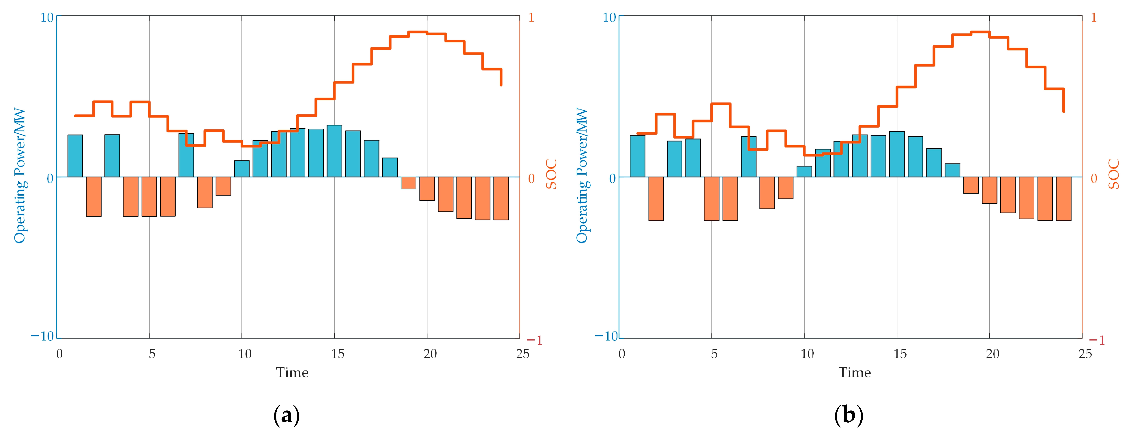
5.2.1. Economic Analysis of Energy Storage Operation

As depicted in Figure 10, the typical daily charging and discharging patterns of the ESS exhibit pronounced peak-shaving and valley-filling attributes. Specifically, the two-node ESS engages in discharging activities during peak electricity price hours from 17:00 to 24:00, facilitating peak-valley arbitrage to augment revenue. It is noteworthy that early morning charging of the ESS aims to capitalize on low electricity price periods, thereby accumulating storage capacity to furnish backup power during ensuing high load periods.

Throughout this process, the SOC of the two grid-connected ESS sites was meticulously maintained within the range of 0.1 to 0.9 to prolong the service life of the energy storage units. Consistently, the ESS exhibits a similar SOC at the outset and conclusion of each day, with a final SOC ranging between 0.3 and 0.5. This meticulous SOC management ensures the continuous operational capacity of the ESS, thereby bolstering the stability and reliability of the overall system.

Table 6. Cost-benefit and Photovoltaic Energy Consumption Rate Comparison under Four Scenarios.

Scenario	Annual Comprehensive Operating Cost/kUSD	Annual Revenue of the Energy Storage System/kUSD	Photovoltaic Energy Consumption Rate/%
1	28.776	—	75.36
2	32.144	—	75.36
3	402.526	60.6035	100
4	368.353	75.155	100

delineates the annual comprehensive operational costs of the active distribution network, the annual revenue generated by the ESS, and the photovoltaic energy consumption rate across four distinct scenarios.

In Scenario 1, the active distribution network operates without an ESS, with photovoltaics providing only active power. The annual comprehensive operation and maintenance cost is approximately USD 28,776. In Scenario 2, the active distribution network also operates without an ESS, but the photovoltaics supply both active power and reactive power compensation to the grid. This increases operational complexity and consumes additional electrical energy, resulting in an annual comprehensive operation and maintenance cost of approximately USD 32,144. Both scenarios lack an ESS for photovoltaic power, leading to a photovoltaic energy utilization rate of only 75.36%, resulting in significant power curtailment. ESSs are needed to smooth photovoltaic power output fluctuations and more sustainably absorb and utilize new energy capacity.

In Scenario 3, the active distribution network does not consider voltage partitioning and installs ESSs at nodes 10 and 28. The annual comprehensive operation and maintenance cost is approximately USD 402,526, and the annual revenue from the ESS is approximately USD 607,722. In Scenario 4, the active distribution network includes ESSs based on distribution network partitioning and voltage layered control. The annual comprehensive operation and maintenance cost is approximately USD 368,353, the annual revenue from the energy storage system is approximately USD 75,155, and the annual operation and maintenance cost is approximately USD 3968. The static investment payback period for the energy storage station is 5.2 years, indicating substantial profit potential for operators investing in shared energy storage stations. Compared to Scenario 3, the overall cost decreases by 8.49%, total revenue increases by 19.36%, and the payback period is further shortened. Both scenarios achieve 100% photovoltaic energy utilization through ESS regulation.

In conclusion, paying service fees to ESS operators for charging and discharging services can significantly reduce user costs. Furthermore, ESS configuration based on regional voltage autonomy is more economical. Simultaneously, the ESS balances power supply and demand through charging and discharging strategies, achieving sustainable utilization of photovoltaic power and zero power curtailment.

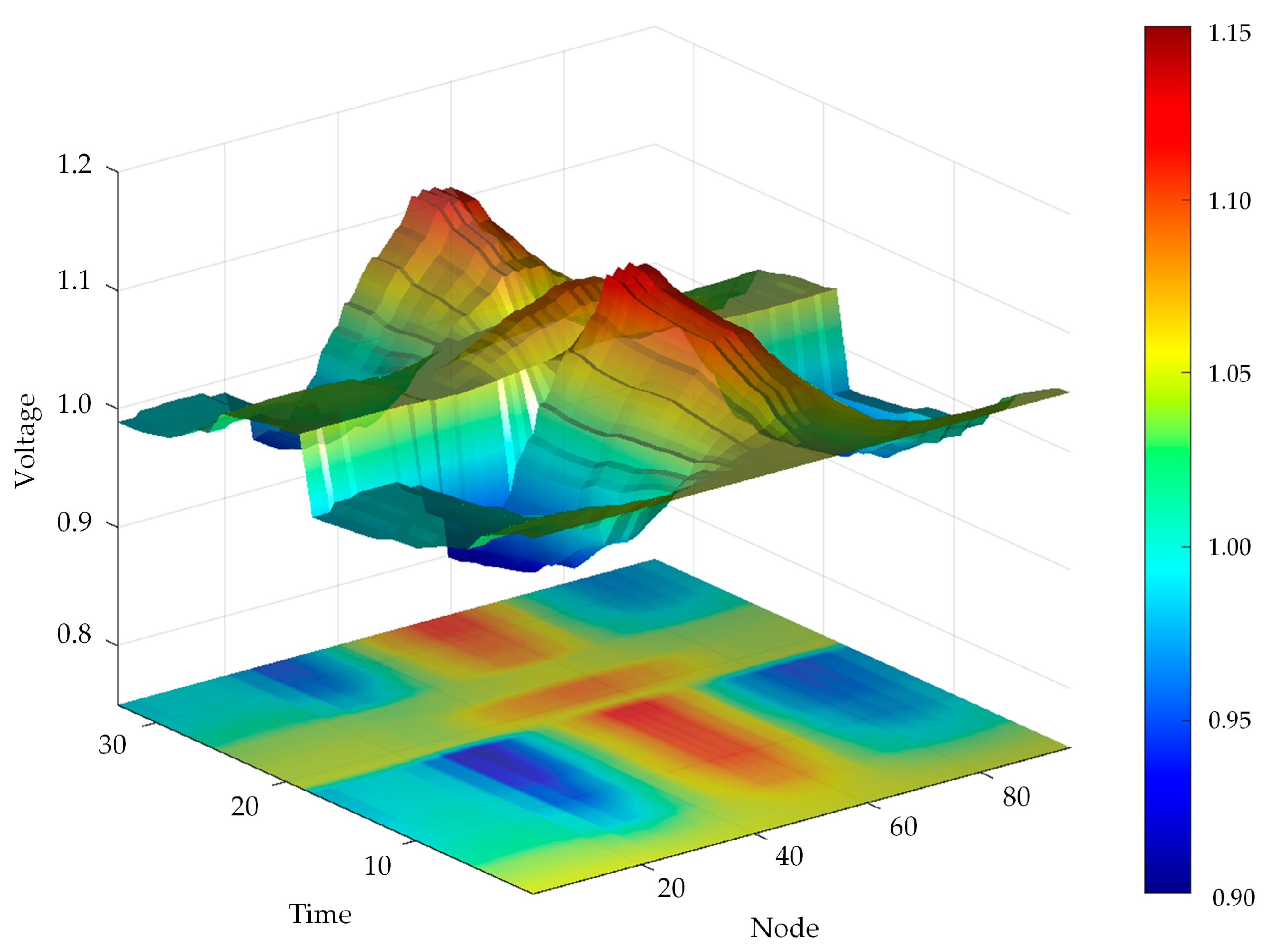
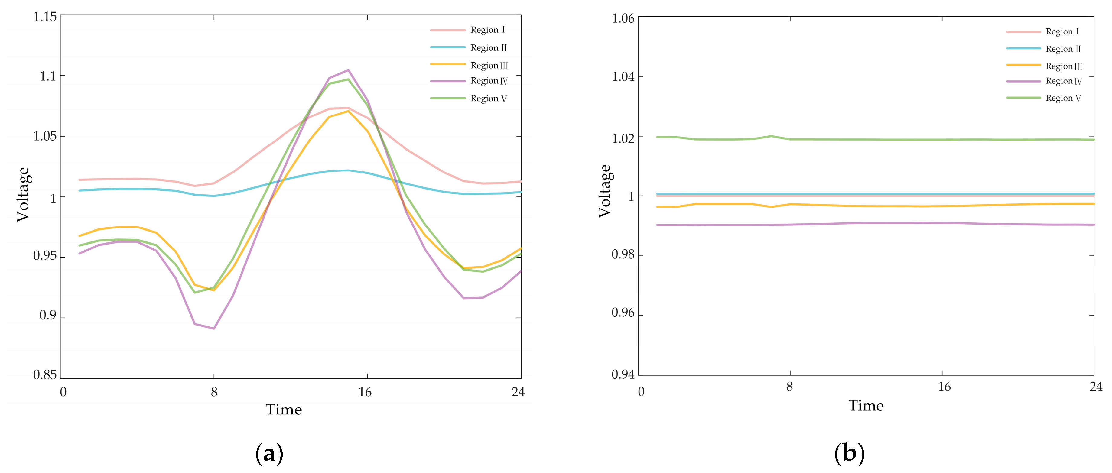
5.2.2. Analysis of Voltage Regulation Effect

In Scenario 1 (Figure 13), there is a voltage rise in the distribution network from 11:00 to 17:00, with the voltage at some nodes in regions R4 and R5 even exceeding 1.10 p.u. Voltage drops occur between 6:00–9:00 and 19:00–23:00, with particularly severe drops at the ends of regions R4 and R5, even falling below 0.90 p.u. At this time, the voltage qualification rate is 90.025%, primarily due to the mismatch between photovoltaic power generation and load demand in both time and space. Therefore, fine voltage regulation is needed during these periods. In Scenario 2, only photovoltaics participate in voltage regulation. From 12:00 to 16:00, the photovoltaic inverter emits inductive reactive power, reducing the voltage of nearby nodes. However, the global voltage cannot be controlled within 1.07 p.u. The main reason is that the photovoltaics are near full capacity, and the reactive power margin input is limited by the inverter capacity. At night, the reactive power margin of photovoltaics is constrained by the power factor, preventing them from providing reactive power support to keep the voltage above 0.93 p.u. At this time, the voltage qualification rate is 94.697%, indicating the need for an ESS for more effective voltage regulation.

In Scenario 3, both PV and ESSs jointly participate in voltage regulation. The ESS mitigates the impact of photovoltaic power fluctuations on voltage through charging and discharging, effectively improving voltage rise and fall phenomena and keeping the voltage within the range of [0.95, 1.05]. In Scenario 4, further consideration was given to regional voltage and weak points, achieving precise voltage regulation with the ESS and keeping the voltage within the range of [0.98, 1.02]. The voltage qualification rate for both scenarios is 100%. Compared to Scenario 3, Scenario 4 further reduces voltage deviation and daily voltage fluctuations at weak points.

Figure 14a illustrates the typical intraday voltage profiles in each region prior to treatment. It is evident that regions IV and V experience substantial voltage fluctuations. Specifically, during the peak sunlight hours at noon, the voltage exceeds the upper limit, while during peak load periods, it falls below the lower limit. The maximum voltage fluctuation at the weakest point exceeds 10%. In contrast, Figure 14b depicts the intraday voltage profiles after the intervention, showing reduced voltage fluctuations and deviations, as well as a decrease in regional voltage disparities. The overall voltage deviation in the distribution network is reduced to 0.217%, indicating effective multi-zone voltage coordination control.

Table 7. Peak Voltage Fluctuations at Weak Points in 4 Scenarios.

Scenario	Node 17		Node 31
	Voltage Deviation	Daily Average Voltage Fluctuation	Voltage Deviation	Daily Average Voltage Fluctuation
1	9.821%	5.846%	9.719%	5.337%
2	8.849%	5.271%	8.365%	4.856%
3	2.487%	0.462%	2.967%	0.055%
4	0.282%	0.251%	1.861%	0.037%

illustrates the gradual improvement in voltage deviation and daily average voltage fluctuation at nodes 17 and 31 with the allocation of resources toward photovoltaic and energy storage management. Both metrics now register at less than 2% and 1%, respectively. Through the combined support of energy storage, active power consumption, and voltage zoning management, the voltage quality at these two weak points has achieved an excellent standard, surpassing national benchmarks.

6. Conclusions

This paper introduces a voltage hierarchical control method based on coordinated active and reactive power management to enhance the regional voltage autonomy of active distribution networks. It establishes a voltage out-of-limit governance model founded on an optimal ESS configuration. By considering the economic and voltage regulation effects across four scenarios, the proposed method is compared and validated within an enhanced IEEE 33-node network. The key findings are summarized as follows.

(i)

The proposed voltage zoning strategy determines the optimal number of reactive areas in the distribution network as five, which are categorized into three types based on reactive power and voltage control capabilities. The algorithm proposed in this paper enhances reactive power modularity by 12.05%, resulting in a more rational voltage region division.

(ii)

The proposed energy storage system configuration model achieves static investment recovery in 5.2 years, indicating that investment in shared ESSs can yield significant profit margins. Compared to scenarios neglecting voltage zoning, its comprehensive costs decrease by 8.49%, while total revenue increases by 19.36%. This optimized configuration strategy notably enhances economic efficiency.

(iii)

The proposed voltage-tiered control strategy improves voltage deviation and daily average voltage fluctuation across distribution network regions under various operating scenarios, thus better serving regional voltage control and enabling 100% local consumption of photovoltaic power.

These research outcomes validate the effectiveness and practicality of the method. Future endeavors by our research team will explore its application in regional integrated energy distribution networks, with forthcoming findings to be reported in subsequent academic publications.

References

1. Wang, S.; Cheng, Y.; Zhao, Q.; Dong, Y. Multi-stage local-distributed voltage control strategy of distribution network considering photovoltaic-energy storage coordination. Electr. Power Autom. Equip. 2024, 44, 1–9. [Google Scholar]
2. Leite, R.; Oleskkovicz, M. The Joint Application of Photovoltaic Generation and Distributed or Concentrated Energy Storage Systems in A Low Voltage Distribution Network: A Case Study. IEEE Lat. Am. Trans. 2023, 21, 1122–1131. [Google Scholar] [CrossRef]
3. Lin, Z.Y.; Jiang, F.; Tu, C.M.; Xiao, Z.K. Distributed Coordinated Voltage Control of Photovoltaic and Energy Storage System Based on Dynamic Consensus Algorithm. In Proceedings of the IEEE IAS Conference on Industrial and Commercial Power System Asia (IEEE I and CPS Asia), Chengdu, China, 18–21 July 2021; pp. 1223–1228. [Google Scholar]
4. Wang, C.Y.; Zhang, L.; Zhang, K.; Song, S.J.; Liu, Y.T. Distributed energy storage planning considering reactive power output of energy storage and photovoltaic. Energy Rep. 2022, 8, 562–569. [Google Scholar] [CrossRef]
5. He, X.; Hashimoto, S.; Jiang, W.; Liu, J.C.; Kawaguchi, T. Design and Implementation of a Low-Voltage Photovoltaic System Integrated with Battery Energy Storage. Energies 2023, 16, 3057. [Google Scholar] [CrossRef]
6. Zou, Y.Y.; Xu, Y.; Feng, X.; Naayagi, R.T.; Soong, B.H. Transactive Energy Systems in Active Distribution Networks: A Comprehensive Review. CSEE J. Power Energy Syst. 2022, 8, 1302–1317. [Google Scholar]
7. Yu, P.; Wan, C.; Song, Y.H.; Jiang, Y.B. Distributed Control of Multi-Energy Storage Systems for Voltage Regulation in Distribution Networks: A Back-and-Forth Communication Framework. IEEE Trans. Smart Grid 2021, 12, 1964–1977. [Google Scholar] [CrossRef]
8. Wang, G.; Wu, X.; Li, L.; Zhang, M.; Li, X.; Cheng, K.; Zhang, J. Optimization method of reactive power and harmonic for photovoltaic multi-function grid-connected inverter under different output states. Electr. Power Autom. Equip. 2024, 44, 80–87. [Google Scholar]
9. Vidhya, K.; Krishnamoorthi, K. A hybrid technique for optimal power quality enhancement in grid-connected photovoltaic interleaved inverter. Energy Environ. 2024, 35, 244–274. [Google Scholar] [CrossRef]
10. Wang, J.; Qin, L.; Xiang, Y.; Ren, P.; Tang, X.; Ruan, J.; Liu, K. A Collaborative Governance Strategy for Power Quality in AC/DC Distribution Networks Considering the Coupling Characteristics of Both Sides. Sensors 2023, 23, 7868. [Google Scholar] [CrossRef]
11. Ge, J.; Liu, Y.; Pang, D.; Wang, C.; Wang, Z.; Liu, Z. Cluster Division Voltage Control Strategy of Photovoltaic Distribution Network with High Permeability. High Volt. Eng. 2024, 50, 74–82. [Google Scholar]
12. Wang, J.J.; Yao, L.Z.; Liu, K.Y.; Xu, J.; Wang, J. Dynamic Regional Division Method of Distribution Network with Regional Autonomy. Power Syst. Technol. 2024, 8, 1–12. [Google Scholar] [CrossRef]
13. Liang, W.; Zhao, Y.; Liu, B.; Wang, Y. Research on Distributed Photovoltaic Low Voltage Ride Through Control Strategy Considering Distribution Network Protection. In Proceedings of the 3rd International Conference on Electrical Engineering and Mechatronics Technology, ICEEMT 2023, Hybrid, Nanjing, China, 21–23 July 2023; pp. 550–555. [Google Scholar]
14. Huang, W.; Liu, S.; Yi, Y.; Wu, Z.; Zhang, Y. Multi-time-scale Slack Optimal Control in Distribution Network Based on Voltage Optimization for Point of Common Coupling of PV. Autom. Electr. Power Syst. 2019, 43, 92–100. [Google Scholar]
15. Zhao, B.; Xu, Z.C.; Xu, C.; Wang, C.S.; Lin, F. Network Partition-Based Zonal Voltage Control for Distribution Networks with Distributed PV Systems. IEEE Trans. Smart Grid 2018, 9, 4087–4098. [Google Scholar] [CrossRef]
16. Lin, Z.; Hu, Z.C.; Zhang, H.C.; Song, Y.H. Optimal ESS allocation in distribution network using accelerated generalised Benders decomposition. IET Gener. Transm. Distrib. 2019, 13, 2738–2746. [Google Scholar] [CrossRef]
17. Liu, J.K.; Zhang, N.; Kang, C.Q.; Kirschen, D.; Xia, Q. Cloud energy storage for residential and small commercial consumers: A business case study. Appl. Energy 2017, 188, 226–236. [Google Scholar] [CrossRef]
18. Liu, J.K.; Zhang, N.; Kang, C.; Kirschen, D.S.; Xia, Q. Decision-Making Models for the Participants in Cloud Energy Storage. IEEE Trans. Smart Grid 2018, 9, 5512–5521. [Google Scholar] [CrossRef]
19. Wu, S.; Li, Q.; Liu, J.; Zhou, Q.; Wang, C. Bi-level Optimal Configuration for Combined Cooling Heating and Power Multi-microgrids Based on Energy Storage Station Service. Power Syst. Technol. 2021, 45, 3822–3829. [Google Scholar]
20. Wang, Y.; Tan, K.T.; Peng, X.Y.; So, P.L. Coordinated Control of Distributed Energy-Storage Systems for Voltage Regulation in Distribution Networks. IEEE Trans. Power Deliv. 2016, 31, 1132–1141. [Google Scholar] [CrossRef]
21. Li, J.; Sun, D.; Zhu, X.; Yu, H.; Li, C.; Dong, Z. Voltage Regulation Strategy for Distributed Energy Storage Considering Coordination Among Clusters with High Penetration of Photovoltaics. Autom. Electr. Power Syst. 2023, 47, 47–56. [Google Scholar]
22. Hen, Z.; Tai, N.; Hu, Y.; Huang, W.; Li, L. A multi-objective joint planning of transmission channel and energy storage system considering economy and flexibility. In Proceedings of the 16th IET International Conference on AC and DC Power Transmission, ACDC 2020, Virtual, Online, 2–3 July 2020; pp. 65–72. [Google Scholar]
23. Li, Y.; Yao, T.; Qiao, X.; Xiao, J.; Cao, Y. Optimal Configuration of Distributed Photovoltaic and Energy Storage System Based on Joint Sequential Scenario and Source-Network-Load Coordination. Trans. China Electrotech. Soc. 2022, 37, 3289–3303. [Google Scholar]
24. Hao, M.; Lan, J.; Wang, L.; Lin, Y.; Wang, J.; Qin, L. Optimized Dual-Layer Distributed Energy Storage Configuration for Voltage Over-Limit Zoning Governance in Distribution Networks. Energies 2024, 17, 1847. [Google Scholar] [CrossRef]
25. Sun, H.P.; Ding, X.H.; Wu, Z.; Wang, K. Voltage Regulation Strategy of Distribution Network Considering Optimization Adjustment of Automatic Voltage Control System Limits. Autom. Electr. Power Syst. 2024, 1, 1–13. [Google Scholar]
26. Li, S.; Wang, Z.; Han, W. A Multi-Objective Current Compensation Strategy for Photovoltaic Grid-Connected Inverter. J. Circuits Syst. Comput. 2022, 31, 2250230. [Google Scholar] [CrossRef]
27. Tian, F.; Huang, L.; Zhou, C.-G. Photovoltaic power generation and charging load prediction research of integrated photovoltaic storage and charging station. Energy Rep. 2023, 9, 861–871. [Google Scholar] [CrossRef]
28. Liao, K.; Pang, B.; Yang, J.; He, Z. Output Current Quality Improvement for VSC with Capability of Compensating Voltage Harmonics. IEEE Trans. Ind. Electron. 2024, 71, 9087–9097. [Google Scholar] [CrossRef]
29. Zhao, P.; Ma, K.; Yang, J.; Yang, B.; Guerrero, J.M.; Dou, C.; Guan, X. Distributed Power Sharing Control Based on Adaptive Virtual Impedance in Seaport Microgrids with Cold Ironing. IEEE Trans. Transp. Electrif. 2023, 9, 2472–2485. [Google Scholar] [CrossRef]
30. Dehghani, N.L.; Shafieezadeh, A. Multi-stage Resilience Management of Smart Power Distribution Systems: A Stochastic Robust Optimization Model. IEEE Trans. Smart Grid 2022, 13, 3452–3467. [Google Scholar] [CrossRef]
31. Jhala, K.; Natarajan, B.; Pahwa, A. Probabilistic Voltage Sensitivity Analysis (PVSA)-A Novel Approach to Quantify Impact of Active Consumers. IEEE Trans. Power Syst. 2018, 33, 2518–2527. [Google Scholar] [CrossRef]
32. Cheng, W.; Gong, G.; Huang, J.; Xu, J.; Chen, K. Decentralized Model Predictive Voltage Control for Distributed Generation Clusters of Power Systems. In Proceedings of the 2023 IEEE IAS Industrial and Commercial Power System Asia, I and CPS Asia 2023, Chongqing, China, 7–9 July 2023; pp. 1615–1619. [Google Scholar]
33. Wand, Z.; Jia, Y.; Li, Y.; Han, X. Optimal Capacity Configuration of Photovoltaic and Energy Storage System in Active Distribution Network Considering Influence of Power Quality. Power Syst. Technol. 2024, 48, 607–617. [Google Scholar]
34. Wu, S.; Liu, J.; Zhou, Q.; Wang, C.; Chen, Z. Optimal Economic Scheduling for Multi-microgrid System with Combined Cooling, Heating and Power Considering Service of Energy Storage Station. Autom. Electr. Power Syst. 2019, 43, 10–18. [Google Scholar]
35. Wen, C.; Mo, J.; Li, J.; Zhou, J.; Wang, P. Coordinate the Optimal Configuration of Double-Layer Hybrid Energy Storage Systems for Wind Farms Participating in Power System Frequency Regulation. In Proceedings of the 10th Frontier Academic Forum of Electrical Engineering, FAFEE 2022, Xian, China, 7–8 December 2022; pp. 97–105. [Google Scholar]
36. Han, R.; Hu, Q.; Cui, H.; Chen, T.; Quan, X.; Wu, Z. An optimal bidding and scheduling method for load service entities considering demand response uncertainty. Appl. Energy 2022, 328, 120167. [Google Scholar] [CrossRef]
37. Zhou, Y.; Wang, J.; Yu, Z.; Liu, W.; Wang, Z.; Kong, W.; Chen, H. Research on Hierarchical Optimization Modeling and Scheduling Technology of Distributed Photovoltaic Cluster. In Proceedings of the 5th Asia Energy and Electrical Engineering Symposium, AEEES 2023, Chengdu, China, 23–26 March 2023; pp. 1438–1443. [Google Scholar]
Figure 1. Schematic Diagram of PV and ESS Integration into Distribution Network Feeder.
Sustainability 16 06758 g001
Figure 2. Distribution Network Voltage Hierarchical Control Method.
Sustainability 16 06758 g002
Figure 3. Schematic Diagram of Typical Radial Network Topology.
Sustainability 16 06758 g003
Figure 4. Flowchart of Regional Optimization Partitioning.
Sustainability 16 06758 g004
Figure 5. Distribution Network Voltage Zoning Strategy.
Sustainability 16 06758 g005
Figure 6. Dual-Layer Optimization Configuration Model.
Sustainability 16 06758 g006
Figure 7. Dual-Layer Model Solving Process Diagram.
Sustainability 16 06758 g007
Figure 8. The IEEE-33 Node Distribution Network with Photovoltaics.
Sustainability 16 06758 g008
Figure 9. Typical Daily Photovoltaic Output Curve for Four Seasons.
Sustainability 16 06758 g009
Figure 10. Division Diagram of the 33-Node Distribution Network.
Sustainability 16 06758 g010
Figure 11. Voltage Fluctuation Curves of Node in the Distribution Network.
Sustainability 16 06758 g011
Figure 12. Voltage Fluctuation Curves of Node in Distribution Network. (a) Node 17; (b) Node 31.
Sustainability 16 06758 g012
Figure 13. Daily Voltage Fluctuations of Distribution Network Nodes in 4 Scenarios.
Sustainability 16 06758 g013
Figure 14. Typical Daily Voltage in Each Region Before and After Treatment: (a) Before Treatment; (b) After Treatment.
Sustainability 16 06758 g014