Article

The Emission-Reduction Effect of Green Demand Preference in Carbon Market and Macro-Environmental Policy: A DSGE Approach

by
Xuyi Ding
1,
Guangcheng Ma
2,* and
Jianhua Cao
1,2
1
Institute of Finance and Economics, Shanghai University of Finance and Economics, Shanghai 200433, China
2
School of Urban and Regional Sciences, Shanghai University of Finance and Economics, Shanghai 200433, China
*
Author to whom correspondence should be addressed.
Sustainability 2024, 16(16), 6741; https://doi.org/10.3390/su16166741
Submission received: 12 July 2024 / Revised: 2 August 2024 / Accepted: 6 August 2024 / Published: 6 August 2024

Abstract

:
Along with the new stage of prevention and control of the COVID-19 pandemic and the vision and goals of combatting climate change, the challenges of the transition to a green economy have become more severe. The need for green recovery of the economy, stability and security of energy production and consumption, and the coordination of low-carbon transformation and socio-economic development has become increasingly urgent. This paper proposes a new theoretical framework to study the effect of carbon emission reduction on the mutual application of the carbon market, fiscal policy and monetary policy under the non-homothetic preference of energy product consumption. By constructing an environmental dynamic stochastic general equilibrium (E-DSGE) model with residents’ non-homothetic preferences, this paper finds that coordinating the carbon market and macroeconomic policies can achieve economic and environmental goals. However, the transmission paths for each are different. The carbon market influences producers’ abatement efforts and costs through carbon prices. Monetary policy controls carbon emissions by adjusting interest rates, while fiscal policy controls carbon emissions by adjusting total social demand. Improving non-homothetic preferences will amplify business cycle fluctuations caused by exogenous shocks, thus assuming the role of a “financial accelerator”. Further research shows that non-homothetic preferences influence the heterogeneity of different policy mixes. Finally, this paper discovers that the welfare effects, the relative size and difference of long-term and short-term effects resulting from the different policy mixes, also depend on the level of non-homothetic preferences. The intertemporal substitution mechanism due to the improvement of non-homothetic preferences endows low-carbon production with “option” characteristics. Our study reveals the role of non-homothetic preferences on the effectiveness of policy implementation. It highlights the importance of matching monetary and fiscal policies with the carbon market based on the consumption and production side. It provides ideas for policy practice to achieve the goal of “dual carbon” and promoting coordinated socio-economic development.

1. Introduction

Nations worldwide have remained resolute in their commitments to addressing climate change despite the impact of the COVID-19 pandemic [1]. Beginning with the goal of “limiting global temperature rise to less than 2 °C” in the Paris Agreement, countries are showing determination for sustainable development in response to climate change [2]. The European Parliament in the European Union approved the “Fit for 55” legislative package (known as Europe’s “biggest carbon market reform in history”) on 18 April 2024. The Legislation includes reforming the Emission Trading Scheme (ETS), amending the rules related to the Carbon Border Adjustment Mechanism (CBAM) and establishing social climate funds. Similarly, in October 2021, China, the world’s highest primary energy consumption and greenhouse gas emission nation, formulated an Action Plan for Carbon Dioxide Peaking Before 2030. China’s national emission trading scheme (carbon market), the world’s largest carbon market, commenced in the same year. Green recovery is crucial to reducing carbon emissions when the world focuses on reviving the economy [3]. The construction of carbon markets of such a scale by the EU and China is bound to be a “shot in the arm” for global action on climate change and economic recovery. However, the low-carbon transition should be rationally viewed to avoid the impact on the regular operation of the economy due to over-aggressive measures such as production cuts and restrictions and to ensure the stability and security of energy production and consumption. Therefore, the problem is how to guide low-carbon transition and economic development in a twin-track way. The main objective of this work is to study whether the carbon market can enable the transformation toward a sustainable low-carbon economic system, guide suitable investments to unlock the benefits and create new jobs to solve social problems and whether it can equitably restructure the economy and society and ensure stability and the long-term benefits of decarbonization, in the context of the increasing public demands for the ecological environment. To answer the questions above, this paper must clarify the mechanisms and effects of different emission-reduction policies and explore the impact of different policy mixes on macroeconomic variables.
Existing studies believe countries implementing carbon markets have different total quotas, covered industries and carbon trading prices, generating certain employment dividends [4]. In order to thrive in a green and low-carbon way, the carbon market is an essential tool for adjusting energy consumption. It ensures a smooth shift in energy supply towards cleaner energy consumption by adjusting the relative prices of different energy sources [5,6]. Consumption behavior changes with income, i.e., preferences are non-homothetic. Thus, the change of relative prices of different energy sources induced by carbon markets will affect household energy consumption and welfare differently [7]. In addition, in monopolistic competitive markets, the demand side will critically affect business cycle fluctuations due to non-homothetic preferences [8]. However, previous studies on energy consumption have focused on single energy preference and price elasticity [9] while ignoring the effects caused by differences in non-homothetic preferences.
In addition to analyzing the emission-reduction effect of the carbon market under non-homothetic preferences, another issue needs to be resolved: Are there any interactions between macroeconomic policies and carbon markets? Domestic macro policies, such as fiscal and monetary policies, aim to promote economic growth [10,11,12,13]. The theoretical logic of the connection between macro policies and carbon markets follows. The carbon emission level of a developing country depends mainly on the total output and the carbon market is built to encourage enterprises to make more efforts or invest more in emission reduction. As a result, firms suffer in the initial period and macro variables are adversely affected. Fiscal and monetary policies mitigate the impact by expanding expenditures and adjusting interest rates, respectively, increasing carbon emissions to a certain extent, thereby offsetting the emission-reduction effect of the carbon market. Figure 1 shows the interest rates, fiscal expenditures and carbon emission growth rates in China from 2001 to 2020. The growth rates of carbon emissions and fiscal expenditures exhibit a similar trend and generally move in the opposite direction to the growth rate of interest rates. The carbon market influences social welfare (including output, consumption and labour) by adjusting the macroeconomic environment, while traditional macroeconomic policies impact carbon emissions as they address economic fluctuations. However, since the introduction of the “dual carbon” goal, the formulation of macroeconomic policies has begun to incorporate this goal. In May 2022, the Ministry of Finance issued the Opinions on Fiscal Support for Carbon Peaking and Carbon Neutrality, proposing that a fiscal and taxation policy framework for green and low-carbon development be gradually established to enhance the guiding role of fiscal expenditure. Regarding monetary policy, the People’s Bank of China introduced a carbon-reduction support tool in November 2021. This tool enables financial institutions to provide loans and interest rate discounts for carbon-reduction projects to enterprises in key areas, with the People’s Bank of China offering credit support amounting to 60% of the loan principal. The one-year interest rate for this support is only 1.75%, compared to the loan market benchmark rate (LPR) of 3.85% for the same period. This indicates that macroeconomic policies are increasingly focusing on environmental pollution, energy conservation and emission reduction, aligning their goals with the carbon market’s goals. This paper argues that when macroeconomic policies and carbon markets are used interchangeably, implementing one policy may affect the effectiveness of the other policy. Currently, research related to macroeconomic policies mainly focuses on evaluating their effects on carbon emission reduction individually [14,15,16,17]. There is little literature assessing carbon-reduction effects when these heterogeneous policies are implemented mutually and even less literature studying the impact of multiple policy applications under non-homothetic preferences on carbon emissions and the underlying mechanisms. Therefore, this paper considers the non-homothetic preferences in reality and examine the emission-reduction effects of the coordinated implementation of carbon markets and fiscal and monetary policies. Our research has significant theoretical and practical implications for guiding countries in achieving their carbon-reduction targets through policy implementation.
Based on the logic above, this paper explores the effect of carbon emission reduction on the mutual application of the carbon market, fiscal policy and monetary policy under non-homothetic energy consumption preferences. Specifically, this paper constructs an environmental dynamic stochastic general equilibrium (E-DSGE) model based on the modeling setting of Annicchiarico and Dio [14] and Blazquez et al. [18]. The model is used to study the impact of carbon market policies, fiscal expenditure policies and price-based monetary policies on carbon emissions under non-homothetic preferences. Moreover, this paper measures the change in households’ welfare caused by policy shocks by constructing a consumption compensation variation (CCV). Understanding the welfare effects of heterogeneous policy shocks also holds essential policy implications. Rational policy choices affect the present and influence the sustainability of smooth production and long-term carbon reduction, which are precisely what welfare analysis involves [19].
In the context of existing literature, this work makes academic contributions in filling the following scientific gaps. (1) From the perspective of non-homothetic preferences, our study delves into how different macroeconomic policy mixes affect carbon emission reduction based on variations in energy demand preferences. Unlike previous studies [8,9,17], this paper is the first to embed non-homothetic consumption preferences into household expected utility functions and construct an E-DSGE model incorporating non-homothetic preferences. This setting helps to make the theoretical model more realistic and discover some results that are not available under the single preference hypothesis. (2) Integrating carbon emission factors into policy functions allows for a study of carbon markets, government departments and central banks taking carbon emissions into account while formulating policies. Current researchers mainly focus on evaluating the impact of macroeconomic policies alone on carbon emission reduction [15,16]. This paper draws inspiration from the Taylor Rule in monetary policy to model policy functions and adjust the response coefficients to carbon emissions, respectively. This approach aims to understand how the three policies—carbon markets, fiscal policy and monetary policy—should respond to varying degrees of macroeconomic shocks and the underlying mechanism, ultimately evaluating which policy mix is most effective in reducing carbon emissions. These settings and tests help to theoretically extend the study of the abatement effects of heterogeneous policy mixes. (3) The welfare effects of carbon emission reduction when the three policies are applied individually and simultaneously are considered in a welfare analysis framework. Previous studies have primarily focused on discussing the welfare effects of a single policy [20,21]. In a single-policy welfare effects analysis framework, it is difficult to “truly” understand the relationship between carbon emission reduction and social welfare. Only an analysis framework incorporating a combination of policies is more realistic, making research about carbon-reduction policy more comprehensive and concrete.
This paper is organized as follows. The following section presents a related literature review. Section 3 formulates the DSGE model. Section 4 is about parameter calibration and estimation. Section 5 analyzes policy shocks’ dynamic effects and mechanisms on vital macroeconomic variables under non-homothetic preferences. Section 6 discusses the welfare changes imposed on households by policy shocks. Conclusions and recommendations are drawn in Section 7.

2. Literature Review

Our study closely relates to two main strands of literature on carbon markets under non-homothetic preferences for energy demand and the carbon abatement effects of macroeconomic policies. Related research is divided roughly into three groups to sort out the overview of research on these two aspects in recent years. The analytical framework of this paper is an extension of the literature on the abatement effects of the carbon market.

2.1. Research Progress on Emission-Reduction Effects of Carbon Markets

The carbon market is an environmental policy based on the market mechanism [22], which has become one of the hot issues in energy and climate research at home and abroad. The discussion on the EU ETS has reached a considerable level of maturity [23,24]. The corresponding literature is also extensive and comprehensive, providing significant references for this paper. The Chinese carbon market has gradually attracted widespread attention from scholars, and some theoretical frameworks have also been established [25]. The main focus has been on the mechanism design, trading operations and economic and environmental impacts [26,27]. However, the research regarding reduction effects is still inconclusive on emission reduction. Many studies have suggested that carbon markets significantly positively affect emission reduction. Li and Ramanathan [28] argue that carbon markets exert cost pressures on polluters and provide economic incentives for them to sell excess emission allowances, adjusting the production patterns of clean and polluting enterprises to enable them to maximize profits and efficiently utilize environmental quotas. Borenstein et al. [15] conclude that carbon pricing policies are crucial for carbon markets to achieve significant carbon reductions, but only sufficiently strong carbon price signals can help achieve carbon neutrality. Zhao et al. [29] point out that the carbon market indirectly affects carbon emissions by optimizing the input of energy intermediates, adjusting energy production and consumption structure and reducing coal consumption. From a micro-firm perspective, Du et al. [30] find that the carbon market significantly reduces firms’ pollution emissions and that cleaner production rather than end-of-pipe treatment plays an essential role in reducing carbon emissions. The results of another group of literature show that carbon market pilots may cause uninvolved regions and participating enterprises to face adverse effects of carbon emission reduction. Tan et al. [31] conclude that China’s ETS pilots shift high-emission and energy-intensive industries to other regions through competition mechanisms and energy demand channels, leading to carbon leakage. Based on the efficient market theory, Wen et al. [32] proposes that irrational behaviors, poor information transparency, imperfect market mechanisms, and high transaction costs cause inefficient carbon emission reductions in different pilot regions. In summary, the conclusions related to the effects of carbon markets on emission reduction are still under discussion, and future research is needed to provide more theoretical and empirical evidence.
Regarding research methodology, current studies on the effects of emission reduction on the carbon market are categorized into three groups. The first group includes research on quasi-natural experiments, which examines the mechanism of ETS pilots in China as an exogenous policy shock that affects carbon emissions [27]. The second group contains research on policy scenario simulation, which analyzes the emission-reduction effect by constructing an emission trading model and designing several policy scenarios, including no emission trading pilot, an emission trading system containing only pilots, a unified carbon market and different tax rates [33,34,35]. The third group provides research on general equilibrium analysis, which assesses changes in factor rewards and distribution of environmental tax reforms in carbon markets through general equilibrium modeling [36]. In recent years, foreign scholars have begun to apply the dynamic stochastic general equilibrium (DSGE) model to the study of environmental problems and have developed the E-DSGE model [14,37]. The E-DSGE model combines the advantages of the DSGE model to avoid the Lucas critique and can be used to study the dynamic effects of different types of stochastic shocks on various variables in the economic system. Therefore, the E-DSGE model is more suitable for studying the effects of stochastic policy shocks in the carbon emission process. Using the E-DSGE model, this paper can embed non-homothetic preferences into the intertemporal utility function of households, thus extending the literature on research methods on the abatement effects of carbon markets.
Heutel [37] first applied DSGE to environmental economics analysis and found that the optimal carbon price should be procyclical. When the optimal carbon price is implemented, carbon emissions will show a procyclical suppression effect. Fischer and Springborn [38] compared carbon taxes and carbon market-related policies and found that the volatility of most macroeconomic variables is small under the emission cap system in the carbon market policy. However, since they all assume that the product market is perfectly competitive and the price level changes at any time, this deviates from the fact that prices are sticky. Then, Annicchiarico and Di Dio [39] constructed an E-DSGE model with price stickiness, focusing on the vital role that price stickiness plays in affecting the effectiveness of carbon market policies. In this regard, the model of this paper also includes the sticky price assumption in Annicchiarico and Di Dio [39]. As the most important innovation of this paper, the setting of non-homothetic preference plays an essential role in scenario research in the DSGE model. Cavallari and Etro [8] argues that the non-homothetic preference nature of goods makes monopolistic competition markets crucial for the demand side effects generated by shock propagation. This effect works through changes in demand for goods within the cycle, primarily through changes in endogenous demand elasticity. The model setting of this paper follows their ideas and extends them into the E-DSGE analysis framework to provide more insights. Regarding modelling heterogeneous producers, Dissou and Karnizova [40] enriches the modelling ideas between final product producers and heterogeneous intermediate product producers by distinguishing between energy and non-energy sectors. The model constructed in this paper also includes the assumption of heterogeneous producers. In addition to carbon market policies, the E-DSGE model in this paper also involves fiscal and monetary policies in the field of the environment. Katircioglu and Katircioglu [41] constructs an E-DSGE model with fiscal policies that include environmental goals and finds that expansionary fiscal policies can alleviate pollution problems. Higher government spending is believed to crowd out private investment, leading to changes in industrial intensity, thereby causing lower carbon emissions. This crowding-out effect of government spending on private investment also applies to this paper’s analysis. The difference between the model constructed in this paper is that a new carbon emission-dependent fiscal policy rule is proposed, which shows how government spending should respond to carbon emissions. Regarding monetary policy, Economides and Xepapadeas [42] introduces energy as a production factor into the production function, focusing on the economic impact of monetary policy shocks that include environmental goals under the E-DSGE model. Unlike their research, this paper only restricts monetary policy to follow specific rules. This paper focuses on which policy combination (carbon market, fiscal, monetary) the policy authorities should adopt to be better.

2.2. Emission-Reduction Effects of Carbon Markets under Non-Homothetic Preferences

Our research supplements the literature on the effects of carbon markets on emission reduction under non-homothetic preferences. In fact, in the analysis of neoclassical economics, people’s consumption preferences and structures can vary significantly due to the differences in income levels and prices. Most previous studies assumed that consumers make homogeneous behavioral choices in the environment. However, in recent years, some literature has analyzed the effects of emission reduction on consumers’ heterogeneous preferences under the impact of policy shocks. The logic is that as higher environmental standards are implemented and consumers shift to environmentally friendly products, manufacturers tend to produce low-carbon products and take measures to suppress carbon emissions [43,44]. For example, Ji et al. [45] construct a Stackelberg model that incorporates supply chain, cap-and-trade regulation and consumers’ low-carbon preferences and find that manufacturers and retailers may accept a cap-and-trade mechanism when consumers have low-carbon solid preferences. Xia et al. [46] consider consumers’ low-carbon awareness in a carbon emission trading system and analyze its impact on manufacturers’ and retailers’ incentives to reduce emissions, profits and utility. The result is that improving consumers’ low-carbon awareness can incentivize manufacturers’ and retailers’ investment in emission reduction, which is conducive to increasing profits and utility. Wang and Wang [47] constructed a carbon market model with carbon tax differences to discuss the impact of consumers’ differentiated preferences for different products on production and emission-reduction decisions. The result shows that the relevant firms will start production only if consumers’ willingness to pay for recyclable products exceeds a certain threshold. Moreover, this threshold also depends on the base tax rate and the preferential tax rate for recyclable products.
In the specific field of the new energy industry, Dogan and Muhammad [48] believe that consumers’ willingness to buy more green electricity or their cheerful willingness to pay a premium for green energy electricity can support the development of green and low-carbon energy. Then, Ndebele [49] uses a random parameter logit model to estimate the choice experiment data of New Zealand electricity consumers online in 2014. The results show that for every 2% increase in the current electricity bill of consumers’ willingness to pay for renewable energy generation, the market share of electricity from renewable resources will increase by 10%. Liobikienė and Dagiliūtė [50] discover that with a new carbon market-related policy, factors such as consumers’ knowledge of green energy, age structure and income level will significantly affect consumption preferences, thereby paying more for green electricity. Cardella et al. [51] subsequently investigate how consumer choice preferences are shifted from traditional to green energy electricity schemes through non-price information, such as generation efficiency under voluntary emission-reduction mechanisms in the carbon market, costs and environmental impacts, to reduce carbon emissions.

2.3. Emission-Reduction Effects of Macroeconomic Policies

The relevant literature on the impact of macroeconomic policies on carbon emissions focuses on three aspects, fiscal policy, monetary policy and the interaction between the two, while the conclusions are inconsistent. Most of the existing literature analyzes the impact of fiscal policy on carbon emissions from the perspectives of taxation, subsidies, carbon pricing and policy mixes. Some scholars believe that fiscal policy will promote carbon emission reduction, while others point out that some fiscal policies will have a negative impact on carbon emission reduction. In fiscal taxation, Rozenberg et al. [16] find that sudden price changes in the short term caused by environmental taxes may lead to stranded assets, which will hit related industries and hinder carbon abatement. In the emission-reduction effect of monetary policy, Sun et al. [17] use green credit policy as a quasi-natural experiment and find that it does not produce a Porter effect within enterprises. The reason is that the green credit policy’s compliance cost and credit constraint effect inhibit firms from innovating. Meanwhile, a green credit policy can prompt enterprises to focus on preventing pollution at the source rather than reducing emissions at the end. Research on the mutual combination of fiscal and monetary policies on carbon emissions is mainly about low-carbon city construction and green finance. The construction of low-carbon cities includes policies such as special funds, industry subsidies and credit incentives to curb carbon emissions by boosting technological innovation levels [52]. The development of green finance includes fiscal measures such as special fiscal funds, fiscal subsidies, fiscal discounts and tax incentives and is also inseparable from structural monetary policy tools. By optimizing the energy consumption structure and substantive green technology innovation, green finance can significantly curb carbon emissions and mitigate the impact of carbon tax policies on the economy, achieving a win–win situation between environmental protection and economic development.

3. The Model

This paper constructs an E-DSGE model that contains six sectors: representative households with non-homothetic consumption preferences, final good producers, intermediate good producers, carbon markets, government and central banks. Among them, representative households with non-homothetic preferences optimize their consumption and labor supply when facing intertemporal budget constraints. Producers, including final and intermediate goods producers, face perfectly competitive and monopolistic competition markets, respectively, and their production results in carbon emissions. Carbon emissions are introduced into the utility function of representative households to explore its social welfare effect. As producers influence carbon emissions, they only affect household utility and do not influence household decision-making. This paper introduces wage stickiness and price stickiness to make the economy more realistic. The carbon market controls the level of carbon emissions through carbon pricing tools. Government departments implement fiscal policies to regulate producers’ carbon emission behaviors. The central bank, on the other hand, regulates carbon emissions through price-based monetary policy.

3.1. Households

Considering the impact of carbon emissions on the utility of a representative household, this paper sets the household utility function as follows:
U C t , L t , C E t = E 0 t = 0 β t ln C t μ L L t 1 + ϕ 1 + ϕ κ ln C E t
This utility function indicates that the consumption of a representative family brings positive utility to it, while providing labor is “painful”, so it brings negative utility to the family. Similarly, the more environmental pollution there is in society, the greater the harm to the health of family members, so it brings negative utility to the family. The budget constraint is:
C t + I t + B t + 1 P t w t L t + r t k u t K t + 1 + i t 1 P t B t + M D t + G t Γ t K t , u t , Z t K t + 1 = 1 δ K K t + Z t 1 γ I 2 I t I t 1 δ K 2 I t
Here, E 0 is the expectation operator based on initial period, β t is the household discount factor and C t is household energy consumption. The coefficient μ L measures the disutility of labor, and ϕ is the inverse of Frisch elasticity. L t is the labor, κ is the parameter of carbon emission disutility and C E t is carbon emissions. I t is the investment, and B t is the investment on riskless bond. w t is the real wage rate, r t k is the real rate of return on capital, while K t is capital stock. i t 1 is the nominal interest rate in t 1 ,   M D t is the profit dividends and G t denotes government fiscal expenditure. This paper defines Γ t K t , u t , Z t as investment adjustment cost, to measure capital adjustment costs incurred in investment. Since capital cannot be adjusted quickly in the short run relative to labor, there is a cost when capital is idle or overutilized. Suppose Γ t K t , u t , Z t K t / Z t λ 1 u t 1 + λ 2 / 2 u t 1 2 , where λ 1 , λ 2 > 0 are parameters for capital utilization costs. λ 2 can be freely calibrated, u t is capital stock utilization for upgrading the model’s endogenous amplification mechanism and Z t is marginal efficiency shock to investment, which follows an AR (1) process: Z t = ρ z Z t 1 + ε z , t . δ K is the capital depreciation rate and γ I is the investment adjustment cost parameter.
Consider the setting of non-homothetic consumption preferences. Drawing on the setting of Cavallari and Etro [8], this paper assumes that a representative household can introduce different types of traditional and low-carbon new energy products into the final set of consumer goods based on the long-term utility achieved from consumption. Thus, the intertemporal utility is represented by a symmetric consumption index:
C t = 0 1 u C t ( i ) d i u
Here, u C t ( i ) is consumption sub-utility, with u C t ( i ) > 0 , u C t ( i ) > 0 and u C t ( i ) < 0 . Under homothetic preferences, this paper first sets the sub-utility function as u ( · ) = ( θ / θ 1 ) C θ 1 / θ , where the elasticity of substitution between products is constant as θ . Second, non-homothetic preferences are introduced. Due to the existence of non-homothetic preferences between households’ choices of traditional energy products and low-carbon new energy products, the elasticity of substitution between products is not constant. Instead, it is influenced by the level of consumption. This paper assumes that the elasticity of substitution between low-carbon new energy products and traditional energy products during the period is given by: θ c = u C t / u C t C t . Bertoletti and Etro [53] believe that θ c can reflect changes in consumption, thus, energy consumption under non-homothetic preferences is C t = 0 1 C i t θ c 1 θ c d i θ c θ c 1 . The preference is given by the following expression:
u C t = ρ C t + θ θ 1 C t θ 1 θ
Here, when the non-homothetic parameter ρ 0 , it satisfies non-homothetic preferences, and the elasticity of substitution during the period can be expressed as θ c = θ 1 + ρ C t 1 / θ . This paper constructs a Lagrangian function for the household utility maximization problem:
L = E 0 t = 0 β t ln ρ C t + θ θ 1 C t θ 1 θ μ L L t 1 + ϕ 1 + ϕ κ ln C E t + λ t w t L t + r t k u t K t + 1 + i t 1 P t B t + M D t + G t K t z t λ 1 u t 1 + λ 2 2 u t 1 2 C t I t B t + 1 P t + ξ t 1 δ K K t + Z t 1 γ I 2 I t I t 1 δ K 2 I t K t + 1
Here, λ t and ξ t are the Lagrange multipliers of the budget constraint and capital accumulation equations, respectively. Define marginal Tobin as q t ξ t / λ t . Households choose consumption (Equation (6)), labor (Equation (7)), capital utilization (Equation (8)), investment (Equation (9)), bond holdings (Equation (10)), and capital stock (Equation (11)) to maximize discounted utility. The first-order conditions of the households’ problem are:
λ t = ρ + C t 1 θ ρ C t + θ θ 1 c t θ 1
L t = λ t w t μ L 1 ϕ
r t k = 1 Z t λ 1 u t 1 + λ 2 u t 1
λ t = ξ t Z t 1 γ I 2 I t I t 1 1 2 γ I I t I t 1 1 I t I t 1 + β E t ξ t + 1 Z t + 1 γ I I t + 1 I t 1 I t + 1 I t 2
λ t = β E t 1 + i t π t + 1 λ t + 1 , π t + 1 P t + 1 P t
ξ t = β E t λ t + 1 r t + 1 k u t + 1 1 Z t + 1 λ 1 u t + 1 1 + λ 2 2 u t + 1 1 2 + ξ t + 1 1 δ K
This paper then assumes that the labor of representative households is also heterogeneous and add wage stickiness to the model. Assume that the labor provided by households is heterogeneous, which gives them the power to bargain for wages and can introduce wage stickiness [54]. The response of total nominal wages to exogenous shocks is weakened, similar to the consistent response of prices and output under price inertia. Consequently, wage stickiness causes the wage markup to exhibit endogenous fluctuations in response to exogenous shocks. However, the assumption of household heterogeneity complicates the utility maximization problem. Since households can earn different wages, they may work varying hours, leading to differences in consumption, bond holdings and, consequently, income. Erceg et al. [54] demonstrated that if complete state-dependent securities exist in the economy and the utility function is additive and separable with respect to consumption and labor, then households will have the same consumption and bond holdings, with only wages and labor varying. Therefore, in the following discussion, it is assumed that state-dependent bonds are present in the economy, which means that consumption and bond holdings are no longer dependent on individual households. According to Calvo [55], households are assumed to have a probability of 1 Φ w Φ w ( 0 , 1 ) per period to adjust the nominal wage to maximize their utility:
max E t s = 0 Φ w β s ( λ t + s W t + s ( i ) 1 + ϕ L t + s ( i ) P t + s Labor income μ L L t + s ( i ) 1 + ϕ 1 + ϕ Labor disutility )
Subject to:
L t + s ( i ) W t + s ( i ) W t + s ε L t + s
where ε is the elasticity of substitution of labor supply, indicating wage markups and distortions in the labor market. The first-order condition of the nominal wage W t ( i ) can be calculated as follows:
E t s = 0 Φ w β s λ t + s ( ε 1 ) W t ( i ) ε W t + s ε L t + s P t + s = E t s = 0 Φ w β s μ L ε W t + s ε ( 1 + ϕ ) W t ( i ) ε ( 1 + ϕ ) 1 L t + s 1 + ϕ Dividing both sides by W t ( i ) ε P t ε ϕ + 1 w t * ε ϕ + 1 = ε ε 1 E t s = 0 Φ w β s μ L W t + s ε ( 1 + ϕ ) π t + s ε ( 1 + ϕ ) L t + s 1 + ϕ E t s = 0 Φ w β s λ t + s W t + s ε π t + s ε 1 L t + s w t * = ε ε 1 E t s = 0 Φ w β s μ L W t + s ε ( 1 + ϕ ) π t + s ε ( 1 + ϕ ) L t + s 1 + ϕ / w t * ε ( 1 + ϕ ) E t s = 0 Φ w β s λ t + s W t + s ε π t + s ε 1 L t + s / w t * ε ε ε 1 s 1 t s 2 t
where S 1 t and S 2 t are two auxiliary wage variables that can be written as recursive equations:
S 1 t = μ L w t w t * ε ( 1 + ϕ ) L t 1 + ϕ + E t s = 0 Φ w β s W t + s ε ( 1 + ϕ ) π t + s ε ( 1 + ϕ ) L t + s 1 + ϕ / w t * ε ( 1 + ϕ ) Let s = k + 1 μ L w t w t * ε ( 1 + ϕ ) L t 1 + ϕ + E t s = 0 Φ w β k + 1 W t + k + 1 ε ( 1 + ϕ ) π t + k + 1 ε ( 1 + ϕ ) L t + k + 1 1 + ϕ / w t * ε ( 1 + ϕ ) = μ L w t w t * ε ( 1 + ϕ ) L t 1 + ϕ + Φ w β E t E t + 1 k = 0 Φ w β k W t + k + 1 ε ( 1 + ϕ ) π t + k + 1 ε ( 1 + ϕ ) L t + k + 1 1 + ϕ / w t * ε ( 1 + ϕ ) = μ L w t w t * ε ( 1 + ϕ ) L t 1 + ϕ + Φ w β E t w t + 1 * w t * ε ( 1 + ϕ ) π t + 1 ε ( 1 + ϕ ) S 1 t + 1
Similarly, the recursive equation for S 2 t can be derived as:
S 2 t = λ t w t w t * ε L t + Φ w β E t w t + 1 * w t * ε π t + 1 ε 1 S 2 t + 1
It can be seen from Equations (15) and (16) that the existence and fluctuation of wage markup actually represent the degree of distortion in the labor market.

3.2. Producers

Assume that there is a representative final good producer in the economy, using continuous energy intermediate goods Y t ( i ) and concluding the final product equation by CES summation:
Y t = 0 1 Y t ( i ) θ 1 θ d i θ θ 1
where θ > 1 represents the incomplete substitution between different intermediate goods. This assumption suggests that intermediate goods producers have pricing power, which is consistent with the reality of the energy market, i.e., the existence of a monopolistic competition market. The demand function of intermediate good Y t ( i ) is Y t ( i ) = P t ( i ) / P t θ Y t , according to the profit maximization problem. Here, P t ( i ) is the price of intermediate goods, and P t is the general price level, which can be expressed as P t = P t ( i ) d i 1 / ( 1 θ ) .
Intermediate goods producers face two problems. The first is the cost minimization problem, subject to the carbon emission constraint. The second is to conduct a dynamic pricing strategy to solve the profit maximization problem under the sticky price. In the first stage, this paper assumes that intermediate goods are produced using existing production technology, capital stock and labor. The production function equals:
Y t ( i ) = ( 1 γ ( C E ) ) A t ( C O V t K t ( i ) ) α L t 1 α ( i )
Here, γ ( C E ) ( 0 , 1 ) is a damage coefficient which captures the impact of carbon emissions on output. According to the definition of Annicchiarico and Dio [14], the higher the carbon emissions are, the higher the damage coefficient will be, with which the environmental impacts caused by carbon emissions are put into the model. A t is productivity for all intermediate good producers, which follows an AR (1) process: A t = ρ A A t 1 + ε A , t . α represents the share of capital. C O V t is the operating rate shock faced by enterprises due to the COVID-19 outbreak, which follows the AR(1) process: C O V t = ρ C O V C O V t 1 + ε C O V , t . This paper refers to the setting of rare disaster risks by Gourio [56] and combines the long shutdown period of enterprises around the world and the decreased willingness of some residents to return to work after the outbreak of COVID-19 to introduce this shock into the manufacturer’s production function to reflect the impact of the inability of enterprises to start work due to shutdowns on economic life.
Carbon emissions from intermediate goods are assumed to be a linear function of their outputs:
C E t ( i ) = χ 1 e t ( i ) Y t ( i )
where χ > 0 is the technological efficiency coefficient of abatement efforts and e t ( i ) is abatement efforts of the intermediate goods producer. There is no carbon emission when the abatement efforts e t ( i ) = 1 . Producers need to pay the corresponding abatement cost to reduce carbon emissions, i.e.,
C E , t ( i ) = ϕ 1 e t ϕ 2 ( i ) Y t ( i )
where ϕ 1 > 0 is the scale coefficient of controlling abatement cost and ϕ 2 is the elasticity of abatement cost to abatement efforts. This form of cost function conforms to the law of increasing marginal cost of abatement as well as ensure the positive effect of carbon tax policy on producers’ abatement efforts in the carbon market. Thus, the producer cost minimization problem is expressed as:
min w t L t ( i ) + r t k C O V t K t ( i ) + C E , t ( i ) + τ t p C E t ( i )
where τ t p is the carbon tax rate faced by producers of intermediate goods. The minimization problems above are subject to the constraints Equations (17)–(20). Construct a Lagrangian function and solve to obtain the producer’s first-order conditions on labor (Equation (22)), capital (Equation (23)), and abatement efforts (Equation (24)):
L t ( i ) = Y t ( i ) A t C O V t 1 γ C E t w t t r t α α 1 α α w t = ( 1 α ) Y t ( i ) L t ( i ) w t 1 α r t k α A t C O V t 1 γ C E t α α ( 1 α ) 1 α ( 1 α ) Y t ( i ) L t ( i ) Λ t
K t ( i ) = w t r t k α 1 α Y t ( i ) A t C O V t 1 γ C E t w t ( k ) t α α 1 α α r t k = α Y t ( i ) K t ( i ) w t 1 α r t k α A t C O V t 1 γ C E t α α ( 1 α ) 1 α α Y t ( i ) K t ( i ) Λ t
e t ( i ) = τ t p χ ϕ 1 ϕ 2 1 Φ 2 1
Equations (22) and (23) are the labor and capital demand curves, respectively, and Equation (24) is the optimal abatement efforts, which depends entirely on the change in the carbon tax, i.e., the higher the carbon tax rate, the harder the producer tries to abate. If the carbon tax rate remains constant, the abatement efforts of the producer is also constant over time. Λ t denotes the real marginal cost of labor and capital subject to environmental constraints. The total marginal cost should equal Λ t plus the marginal cost of abatement and the marginal cost of paying the carbon tax:
M t ( i ) = Λ t + ϕ 1 e t ϕ 2 ( i ) + τ t p φ 1 e t ( i )
Then this paper considers the profit maximization problem. Since the energy market is imperfectly competitive, the producer of the intermediate good has the pricing power. The price is set by price markup: P t ( i ) = θ θ 1 M t ( i ) . Assuming that intermediate good producers discount their future profits using the same stochastic discount factor:
S D F t + s = β s U ˙ c t + s U c t
Consider the pricing strategy of intermediate good producers. In order to introduce sticky prices, significant exploration has been conducted in the literature. Classic models of sticky prices typically assume that in each period, a fraction 1 / t of manufacturers can re-price, with the number of manufacturers allowed to re-price decreasing as t increases. However, the staggered pricing mechanism based on this strategy makes model aggregation, that is, removing heterogeneity, extremely cumbersome. Drawing on the staggered pricing mechanism proposed by Calvo [55] to introduce price stickiness: assuming that any producer has a fixed probability of 1 Φ p Φ p ( 0 , 1 ) in each period to adjust the price, which does not change over time. Logically, this staggered pricing mechanism is straightforward, and from a technical standpoint, it simplifies the aggregation process (eliminating heterogeneity). Over time, it has evolved into the most classic and commonly used staggered pricing mechanism and a standard component in DSGE model. Assuming that intermediate good producers can adjust prices in period t but cannot adjust prices in all subsequent periods, the optimal price, P t ( i ) , can be chosen to maximize the profit as follows:
max E t s = 0 Φ p β s U c t + s U c t ( P t + s ( i ) 1 θ Y t + s θ 1 Real income M t + s P t + 1 P t + s Real cost )
The first-order condition with respect to P t ( i ) is:
P t ( i ) θ E t s = 0 Φ p β s U c t + s U c t ( 1 θ ) P t + s θ 1 Y t + s + θ M t + s P t ( i ) 1 P t + s θ Y t + s = 0 P t * = θ θ 1 E t Σ s = 0 Φ p β s U c t + s M t + s P t + s θ Y t + s E t s = 0 Φ p β s U c t + s P θ 1 Y t + s Y t + s θ θ 1 X 1 t X 2 t
From the above first-order conditions, the price choice of intermediate producers is independent of the index. Therefore, all intermediate product manufacturers choose the same optimal adjustment price, and the choice is symmetrical. Therefore, j can be removed to show symmetry. X 1 t and X 2 t are two auxiliary variables that can be written as recursive equations:
X 1 t = U C t M t Y t + E t s = 1 Φ p β s U C t + s M t + s P t + s θ Y t + s Let s = k + 1 U C t M t P t θ Y t + E t s = 1 Φ p β s U C t + s M t + s P t + s θ Y t + s = U C t M t P t θ Y t + E t k = 0 Φ p β k + 1 U C t + k + 1 M t + k + 1 P t + k + 1 θ Y t + k + 1 = U C t M t P t θ Y t + Φ p β E t E t + 1 k = 0 Φ p β k U C t + k + 1 M t + k + 1 P t + k + 1 θ Y t + k + 1 = U C t M t P t θ Y t + Φ p β E t X 1 , t + 1
Similarly, the recursive equation for X 2 t can be derived as:
X 2 t = U C t P t θ 1 Y t + Φ p β E t X 2 , t + 1
The above equation implies a classic conclusion: under elastic prices, the price chosen by a monopolistic competitor is equal to a markup on the (nominal) marginal cost. To get the equilibrium conditions, the inflation rate and auxiliary variables are defined as:
π t * P t * P t 1 * , x 1 t X 1 t P t θ , x 2 t X 2 t P t θ 1
This paper have:
π t * = θ θ 1 π t x 1 t x 2 t
x 1 t = λ t M t Y t + Φ p β E t x 1 , t + 1 π t + 1 θ
x 2 t = λ t Y t + Φ p β E t x 2 , t + 1 π t + 1 θ 1
Based on the demand and production functions of intermediate goods, the sum of the labor and capital demand functions gives:
0 1 Y t ( i ) d i = 0 1 P t ( i ) P t θ Y t d i Y t = 0 1 Y t ( i ) d i 0 1 P t ( i ) P t θ d i d t P 1 ( 1 γ ( C E ) ) ( C O V t K t ( i ) ) α L t 1 α ( i ) d i = d t P 1 ( 1 γ ( C E ) ) A t ( C O V t K t ( i ) ) α L t 1 α
where d t P is a price discretization kernel, measuring price dispersion. A larger d t P indicates a greater dispersion of P t ( i ) . d t P indicates that the manufacturers that can readjust prices in each period are randomly selected, and there are a large number of intermediate product manufacturers. Therefore, the integral on a subset of [0, 1] should be proportional to the integral of the entire interval [0, 1], and this proportion is exactly the length of the subset. The staggered price mechanism is introduced into the discretization kernel and written in the following recursive form:
d t P = 0 1 θ P t * P t θ d i + 1 θ 1 P t 1 ( i ) P t θ d i = 1 Φ p 0 1 P t * P t θ d i + Φ p π t θ 0 1 P t 1 ( i ) P t 1 θ d i 1 Φ p π t * θ π t θ + Φ p π t θ d t 1 P
According to P t = P t ( i ) d i 1 / ( 1 θ ) and π t * = P t * / P t 1 , the following equation holds when there is no inflation:
0 1 P t ( i ) P t θ d i = 1 Φ p P t * P t 1 θ P t P t 1 θ + Φ p P t P t 1 θ 0 1 P t 1 ( i ) P t 1 θ d i 0 1 P t ( i ) P t θ d i P t P t 1 θ 0 1 P t 1 ( i ) P t 1 θ d i = 1 Φ p P t * P t 1 θ 0 1 P t 1 ( i ) P t 1 θ d i + Φ p π t 1 θ = 1 Φ p π t * 1 θ + Φ p
A first-order logarithmic linearization of the above equation yields:
π ˜ t = ( 1 Φ ) π ˜ t *
where π ˜ t * = log P t * log P t 1 . Equation (38) shows that the optimal choice of intermediate good producers’ adjustable prices, is not the weighted average price of the previous period, thus leading to inflation. Furthermore, the equation shows that when perfect price stickiness prevails, net inflation is zero.
Based on the above results, the total carbon emissions level and the total abatement costs are obtained by summing up:
C E t = χ 1 e t Y t d t P
C E , t = 0 1 C E , t ( i ) d i = ϕ 1 e t ϕ 2 Y t d t P
The budget constraint on the final good (i.e., market clearing) is expressed by:
Y t = C t + I t + G t + C E , t + γ I 2 I t K t δ K 2 C O V t K t

3.3. Carbon Markets

The core issue of carbon market policy is carbon pricing. Carbon pricing can encourage changes in production patterns by incorporating the costs of climate change into individual economic decisions through price signals. Currently known carbon pricing models can be categorized into explicit and implicit carbon pricing. Explicit carbon pricing mainly includes a carbon tax, carbon emission trading system, carbon credit mechanism, shadow carbon price and internally negotiated pricing. Carbon tax and ETS are currently the most widely used carbon pricing tools. The core of the current carbon emission trading system’s pricing mechanism is the same as the carbon tax mechanism, that is, by charging carbon fees for carbon emissions. In contrast, the pricing subject has been changed from the government to the market, and quotas have been allocated accordingly. Therefore, this paper redefines τ t p as the carbon price under the carbon market policy.
This paper assumes that the carbon market controls pricing in the current period based on the carbon emissions and carbon price of the previous period, and satisfies the following rules:
ln τ t p , d = 1 ψ τ ln τ p ¯ + ψ τ ln τ t 1 p , d + 1 ψ τ ψ c e ln C E t C E ¯ + ε τ , t
Here, τ ¯ p ¯ is the steady-state level of carbon price. 0 < ψ c e , ψ τ < 1 is the response to carbon emissions and carbon price when the carbon price policy is implemented, which describes the persistence of the policy shock. ε τ , t represents the carbon price policy shock normally distributed with mean zero and standard deviation σ τ . Equation (42) assumes that economic agents in the market expect to maintain carbon emissions at the target steady-state value through carbon price tools. The carbon market will automatically increase the carbon price if the actual carbon emission exceeds the target value. However, to avoid excessive changes in carbon prices, the carbon market adopts market stability reserves, price corridors, emissions control reserves, auction floor prices and cost control reserves. This suggests that the carbon market only sets the carbon price policy at a biased constant value τ t p , d .

3.4. Central Banks

Since the carbon emissions function is linear with output, this paper draws on the standard Taylor rule’s setting and ignore the money supply’s impact. Assume that the central bank adopts a smooth price-based monetary policy and determines the current interest rate based on the previous period’s interest rate, inflation, output and carbon emissions. This results in the following function:
ln i t = 1 ψ r ln ( i ) + ψ r ln i t 1 + 1 ψ r ψ π ln π t 1 π ¯ + ψ Y ln Y t Y t 1 + ψ m ln C E t C E ¯ + ε r , t
where i ¯ , π ¯ and Y ¯ are the steady-state interest rate, inflation and output, respectively. ψ r , ψ π , ψ Y and ψ m are the degrees of response to interest rate, inflation, output and carbon emissions, respectively, when the central bank implements price-based monetary policy, which describes the persistence of the policy shocks. The monetary policy shock ε r , t is normally distributed with mean zero and standard deviation σ r . The theoretical logic behind Equation (43) is that by raising interest rates, the central bank will increase household savings and curb consumption, leading to a decline in demand, price and output and reducing carbon emissions.

3.5. Government

Unlike the carbon market, the government is motivated to strengthen the traditional administrative intervention of fiscal policy tools to regulate carbon emissions under the constraints of carbon emission-reduction targets since the carbon market has not yet been perfected. Therefore, this paper assumes that the government plays a role in fiscal policy through government fiscal expenditures and carbon pricing charges. This paper sets the proportion of government fiscal expenditures to output as G E t g , and the equilibrium condition for the government sector is derived as follows:
G t = G E t g Y t + τ t p , d C E t
Similarly, assuming that the government determines the current period’s expenditure share based on the previous period’s fiscal expenditure share and carbon emissions, the following rule is satisfied:
ln G E t g = 1 ψ g ln ( G E ¯ ) + ψ g ln G E t 1 g + 1 ψ g ψ g m ln C E t C E ¯ + ε g , t
where G E ¯ is the steady-state level of the government expenditures share. 0 < ψ g , ψ g m < 1 , respectively, refer to the degree of responsiveness to government spending and carbon emissions when the government implements fiscal policy and describes policy shock persistence. ε g , t represents the fiscal policy shock that follows a normal distribution N 0 , σ g .

4. Calibration and Estimation

The parameters in this paper include parameters outside the model (structural parameters) and parameters inside the model (policy-related parameters). This research uses previous literature, statistical data, common sense settings and other means to calibrate structural parameters. At the same time, policy-related parameters are often obtained by estimation using Bayesian methods since they are difficult to acquire by statistical data.

4.1. Calibration

The structural parameters that need to be calibrated in the E-DSGE model in this paper mainly include the following: Consider the household discount factor β . The inflation is zero in the steady state, that is, π = 1 . According to i = π / β , β value of 0.99 means that the annual riskless interest rate and also implies that the model corresponds to a quarterly frequency of data. The labor disutility parameter μ L is calculated by steady state. According to common practice in the literature, the inverse of the Frisch elasticity of labor supply is set to 1, indicating that wages and labor supply grow at the same rate [57]. Zhang and Zhang [58] estimate the environmental effect elasticity of representative households, and the estimated value is 0.20. Thus, this paper sets the carbon emissions disutility parameter κ to 0.20. Assuming that capital is depreciated by 10 % per year, the quarterly capital depreciation rate, δ K , is 0.025. The investment adjustment cost parameter, γ I , is the degree of sensitivity of investment to the marginal Tobin’s Q. The smaller the value, the greater the sensitivity, that is, a slight change in cost can cause a significant change in investment. Most of the existing literature sets the range of values of the investment adjustment cost parameter γ I as [ 1 , 3 ] [59,60,61], which set to 2.00. The capital utilization cost parameter λ 1 is calculated by steady state and λ 2 can be calibrated freely. When λ 2 is set too large, it leads to a lower output response to exogenous shocks, and a value of 0.01 is generally sufficient [57]. The elasticity of substitution between clean energy and traditional energy products has been adopted primarily following Annicchiarico and Diluiso [59] and Pan et al. [60]. This paper sets the elasticity θ = 6.00 . Also, assuming the household wage markup is 20 % , the supply substitution elasticity of labor ε is 6.00. Referring to Bertoletti and Etro [53], the non-homothetic parameter ρ is set to 1.00. According to Calvo [55] staggered pricing mechanism, when the wage stickiness parameter Φ w and the price stickiness parameter Φ p are 0.75, prices remain unchanged for four quarters, which is in line with our setting of a quarterly benchmark period. This paper align with Annicchiarico and Diluiso [59] in establishing the share of capital output α as 1 / 3 . As Heutel [37] calculated, this paper sets the damage coefficient of emissions as 0.0026. This research follows Annicchiarico and Dio [14] by setting the technological efficiency factor for abatement efforts χ as 0.45, the scale coefficient of controlling abatement costs ϕ 1 as 0.185 and the elasticity of abatement costs to abatement efforts ϕ 2 as 2.80. Moreover, as in Chan [62], this paper sets the steady-state carbon price of the carbon market and the steady-state level of government expenditure proportion to 0.05 and 0.20, respectively. The calibration results of specific parameters are shown in Table 1.

4.2. Bayesian

In the estimation process, this paper uses five observable sequences: the real GDP, real investment, real consumption, labor force and inflation rate of the United States. Among them, real GDP, real investment and real consumption are estimated from nominal values and GDP deflator and CPI measures the inflation rate. The data are from the International Monetary Fund and span the period from the first quarter of 2000 to the fourth quarter of 2023. All data are deseasonalized and detrended using the Census X12 method and HP filtering.
In the carbon market policy, the prior distribution of the carbon price response coefficient ψ τ is assumed to be Beta distributed, which is set to a mean of 0.5 and a standard deviation of 0.10. Drawing on the monetary policy rules, this paper sets the prior distribution ψ c e of response coefficient to carbon emissions as a normal distribution with a mean of 1.50 and a standard deviation of 0.10 [60]. In monetary policy, this paper follows Annicchiarico and Diluiso [59] to assume that the prior distribution of response parameter of monetary policy to interest rates ψ r is Beta distributed with mean 0.50 and standard deviation 0.20 to inflation ψ π is normally distributed with mean 1.60 and standard deviation 0.10 and to output ψ Y is normally distributed with mean 0.10 and standard deviation 0.05. Referring to Noureen et al. [63], the prior distribution of the response parameter of monetary policy to emissions ψ m is normally distributed at a mean of 0.12 and a standard deviation of 0.20. In fiscal policy, the prior distribution of the response parameter of fiscal policy to government spending ψ g is assumed to be Beta distributed with a mean of 0.50 and standard deviation of 0.20. Following Noureen et al. [63], the prior distribution of the response parameter of fiscal policy to emissions ψ g m is assumed to be normally distributed with a mean of 0.05 and a standard deviation of 0.02. The prior distribution of the autoregressive parameters of investment efficiency shock and technology shock is a beta distribution, of which the mean and standard deviation are set to be 0.70 and 0.20, respectively. This paper assigns values to the five exogenous shocks in the model (investment efficiency shock ε z , t , technology shock ε A , t , carbon price policy shock ε τ , t , monetary policy shock ε r , t and fiscal policy shock ε g , t ) following the estimation results of the observable series [59,60,63]. This paper follows the approach of Gourio [56] and assumes that the ρ C O V follows a beta distribution with a mean of 0.50 and a standard deviation of 0.02 and ε C O V , t follows an inverse gamma distribution with a mean of 0.02 and a standard deviation of 2.
Since the posterior distributions of economic parameters cannot be expressed in the analytical form in most DSGE models and thus cannot be computed by Bayes’ law, the posterior distributions can only be approximated by the Monte Carlo method through random sampling. Therefore, this paper uses Markov Chain-Monte Carlo (MCMC) and Metropolis-Hastings Algorithm to simulate the posterior distribution. This paper uses Kalman filtering to estimate the likelihood function in combination with the observed data. Then, the maximum value of the likelihood function is derived using the numerical solution algorithm. Finally, simulated by the MH algorithm, which extracts the Markov chain and approximates the density of the posterior distribution by histogram approximation, the posterior distributions are obtained. The estimation results of the parameters are shown in Table 2.

5. Dynamic Analysis and Mechanisms

In this part, this paper uses Matlab R2024a and Dynare 4.5.0 software to conduct numerical simulations of the three policy matching scenarios to examine the dynamic impacts and transmission mechanisms of different policy shocks on key macroeconomic variables under non-homothetic preferences.

5.1. Analysis of the Transmission Path of Carbon Price Shocks

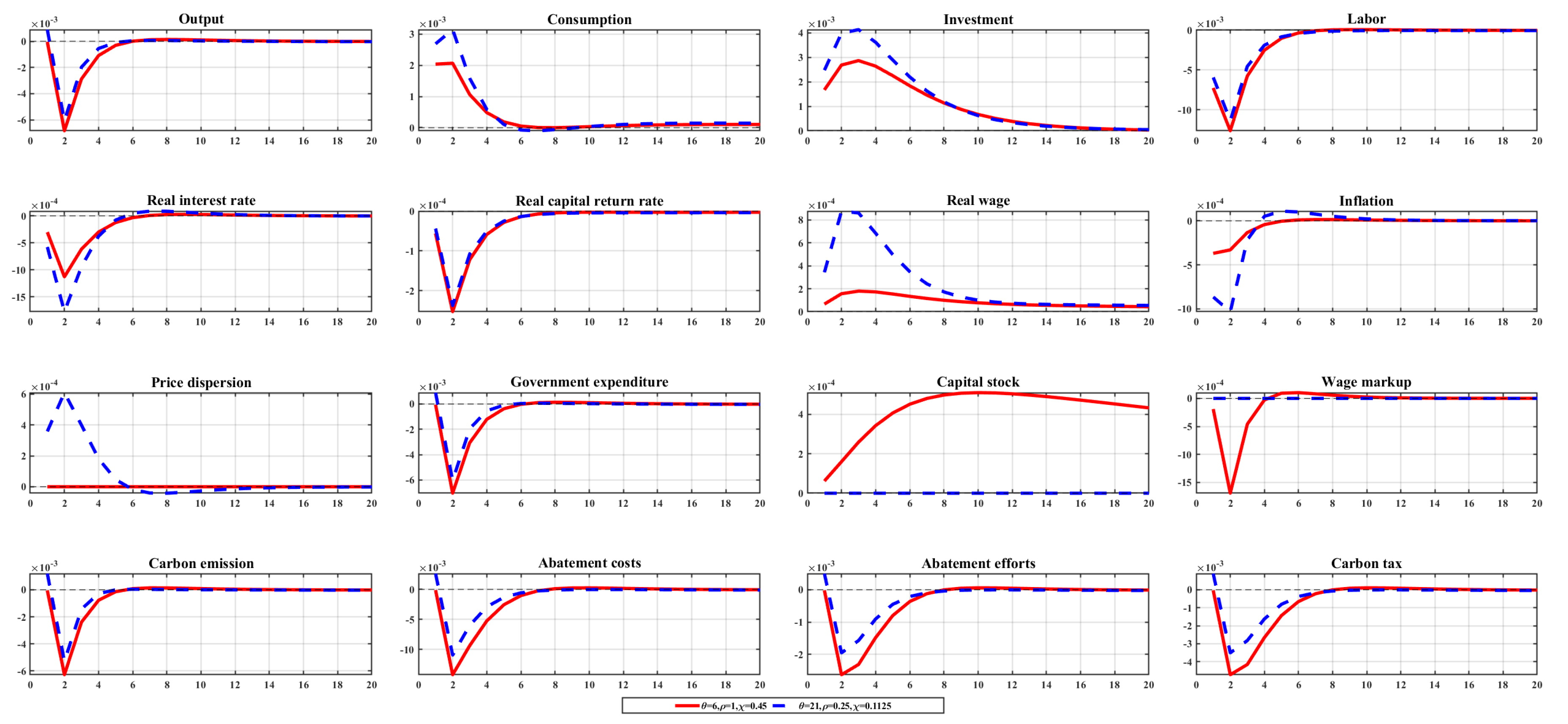
Figure 2 shows the impulse response functions of a positive carbon price policy shock on output, consumption, investment, labor, the nominal interest rate, the real rate of return on capital, the real wage, inflation, carbon emissions, the abatement cost, the abatement efforts and the carbon tax under non-homothetic preferences. The solid lines are obtained with a higher elasticity of substitution for energy products, non-homothetic preference and technological efficiency of abatement efforts, while the dashed lines are about the low situation. This paper analyze the policy’s long- and short-term dynamic impacts by treating the first four periods of post-shock changes as short-term impacts and the fifth to the twentieth periods as the long-term impacts of the shock.

5.1.1. Impact of Carbon Price Shocks

In terms of the magnitude of the impact, when an economy is hit by a positive carbon price policy shock, output, consumption, investment, labor, the real rate of return on capital, the real wage, inflation, government spending, the capital stock, the wage markup, the cost of abatement, the level of abatement efforts and the carbon tax will show an upward trend. In contrast, the nominal interest rate and carbon emissions show a downward trend.
On the production side, when a positive carbon price policy shock increases the carbon tax rate, producers will make more efforts to abate, as shown by the first-order condition of abatement efforts (Equation (24)). Government spending also rises with the rise in the carbon tax, as shown in Equation (44). In maintaining the same level of output, producers will face higher abatement costs (i.e., as shown in Equation (20)). Therefore, producers of energy consuming intermediate goods will tend to reduce carbon emissions in order to ensure cost minimization (Equation (21)). On the consumption side, representative households are more inclined to consume low-carbon new energy products due to the characteristic of non-homothetic preference. Low-carbon new energy products produced by producers in the process of carbon emission reduction will be favored by representative households. Meanwhile, the increase in producers’ abatement costs and investment adjustment costs will stimulate the demand for low-carbon intermediate and final products.
Thus, the final output increases due to the interaction between the low-carbon intermediate and final goods demand. The increase in low-carbon new energy products generates a positive consumption utility for non-homothetic representative households, leading to an increase in consumption in the household sector. Producers of low-carbon intermediate goods need to invest more in labor due to the increased supply capacity of their products, causing the labor and real wages and wage markups to rise. Under the interest burden, the increase in inflation is accompanied by a decrease in nominal interest rates, which will bring a fall in real interest rates. The decrease in real interest rates leads to a fall in the real cost of debt for producers, i.e., a rise in net worth, a fall in the risk premium on external financing, a rise in the real rate of return on capital and a corresponding rise in investment and the capital stock.

5.1.2. Impact Cycle of Carbon Price Shocks

In terms of the impact cycle, the impact of carbon price policy shocks on output, consumption, labor, the real interest rate, the rate of return on capital, inflation, government spending, wage markups, carbon emissions, the abatement costs, the abatement efforts and the carbon tax in an economy is basically within four periods. It gradually tends to a steady state after the fifth period. As is shown in the gross emissions function C E t = χ 1 e t Y t d t P , when the carbon emission intensity of a unit of output is given, the price dispersion core under the staggered pricing mechanism increases. Due to price stickiness, carbon emissions caused by reducing one unit of the final product will require more low-carbon intermediate inputs. Therefore, high abatement efforts are not needed in the long run, and abatement costs and carbon emissions tend to stabilize in the long term.
However, the carbon price policy has long-run effects on investment, capital stock and real wages, with investment converging to a steady state after the 15th period and real wages remaining above the steady state level for a long time. In the short run, investment, the real interest rate and real wages all peak around periods 2 and 3. Output rises when consumption increases, leading to increased producer profits, labor income and a slight price increase. Since investment takes time to adjust, and over the long term, non-homothetic will make consumption demand slightly above the steady state; investment will be higher than the steady state in the long run. The increase in investment brought about by the shock will cause an increase in capital available to producers and a sustained increase in the capital stock, which will raise factor production capacity. With the triple combination of the higher marginal output of labor, lower general price and sticky wages, finally, real wages continue to be higher than the steady-state level in the long run.

5.1.3. Impact of Carbon Price Shocks under Low Non-Homothetic Preferences

The impact of carbon price policies shows heterogeneity under different settings, that is, the effects of shocks are influenced by the elasticity of substitution between low-carbon new energy products and traditional energy products, non-homothetic parameters and the technological efficiency of abatement efforts. As the elasticity of substitution decreases, the non-homothetic parameter decreases and the technological efficiency of the abatement efforts diminishes, the effects of the shocks diminish for all economic variables except inflation. The reason is that the sticky parameter causes price dispersion in the economy. The larger the sticky parameter, the stronger the degree of price dispersion and, therefore, the higher the inflation. In the lower case, price dispersion shows a downward trend, indicating that the degree of price dispersion decreases and the level of inflation subsequently decreases. Increased elasticity of substitution amplifies cyclical fluctuations because the intertemporal substitution effect incentivizes households to anticipate high consumption and a more excellent labor supply during booms when prices are relatively low and wages are relatively high.
The new low-carbon energy products brought about by the carbon price policy shock are not effectively consumed at lower elasticity of substitution, non-homothetic, and technological efficiency of abatement efforts. Producers often have to pay the same abatement costs and abatement efforts as when the elasticity of substitution is high, which raises the cost of production and ultimately leads to higher cost-driven inflation at the beginning of the period. At the same time, the elasticity of demand resulting from the elasticity of substitution under a set of non-homothetic preferences varies with the level of consumption. It induces producers to change their desired price markup in response to the shock. Higher elasticity of substitution and non-homothetic preferences allow more and more producers to commit to desiring and innovating energy-efficient products in response to positive carbon tax shocks, thereby increasing the technological efficiency of abatement efforts and ultimately reducing carbon emissions. Although producers need to weigh the costs and benefits of shifting to cleaner production, when consumers have high preferences for low carbon, producers will move away from short-term interest to a sustainable business model [43]. Thus, the non-homothetic preferences of representative households for low-carbon new energy products are a crucial mechanism through which carbon pricing policies work and exacerbate the degree of responsiveness of non-production-side economic variables.

5.2. Analysis of the Transmission Path of COVID-19 Shocks

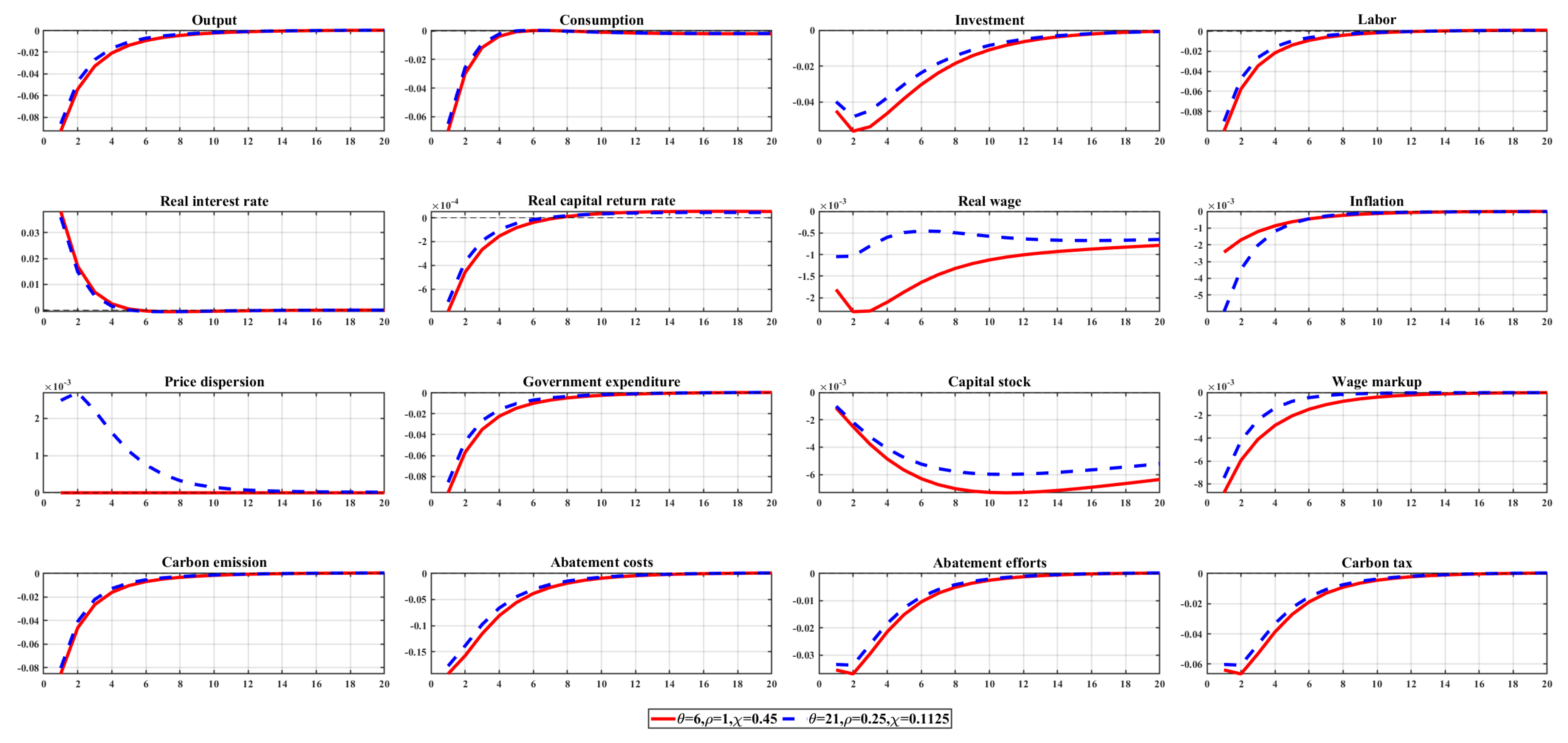
Figure 3 illustrates the economic impact of the COVID-19 shock. The positive COVID-19 impact led to a substantial drop in output. However, output is expected to return to its original level after six periods, reflecting that the occurrence of the disaster will indeed have a more lasting impact on normal economic production. At the same time, the labor supply will also be affected, showing a significant decline that will take a long period to recover. This indicates that the impact of COVID-19 will have a notable negative effect on the entire society. Regarding investment, reductions in employment and production will lower the marginal product of capital, thus decreasing total investment demand. However, due to factors such as the impact of rare disasters, the bankruptcy of old companies, the establishment of new companies and government bailouts, total investment will quickly surpass its original level, leading to a rise in real interest rates and capital prices after a brief decline. The reduction in production means that enterprise emissions will also decrease rapidly, reducing the intensity of emission-reduction efforts and alleviating the burden of emission-reduction costs. Consequently, the transaction volume in the carbon market decreases, leading to a lower level of carbon tax. However, since the COVID-19 shock is not the focus of this study, the impact of the COVID-19 shock is no longer considered in subsequent policy combinations and welfare analysis.

5.3. Analysis of the Transmission Path of Monetary Policy Shocks

Unlike carbon pricing, price-based monetary policy sets the current interest rate through the previous period’s nominal interest rate, inflation, output and carbon emissions level. The central bank becomes a “modified” Taylor rule by linking carbon emissions to the nominal interest rate.

5.3.1. The Impact and Cycle of Monetary Policy Shocks

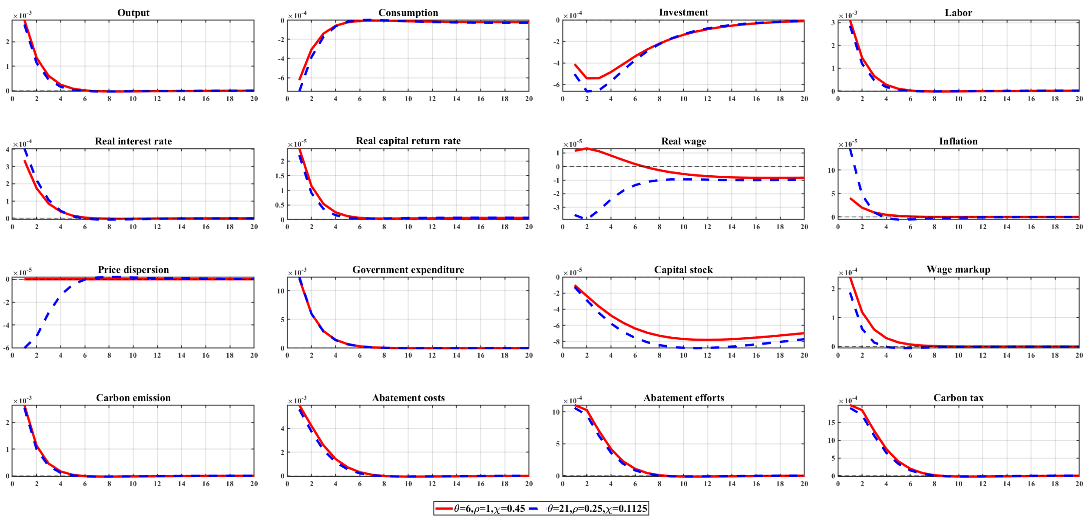
Figure 4 shows that in the short run, a positive monetary policy shock increases nominal interest rates and encourages household savings while discouraging household consumption, real investment and capital stock and increases the cost of external financing for producers, leading to lower output and carbon emissions levels. The abatement mechanism under monetary policy shocks differs from the carbon price policy in that the former has negative shocks to the carbon tax, the abatement efforts and the abatement cost. That is, monetary policy does not enable producers to autonomously increase their abatement efforts and thus increase the cost of abatement to reduce carbon emissions. Instead, demand is dampened by adjusting the nominal interest rate, which causes producers to hire less labor and rent less capital, leading to a decline in wages and the real rate of return on capital.
Policy shocks result in a decline in the carbon tax because the tax is pro-cyclical, and carbon tax policymakers tend to iron out the tightening effect of monetary policy on output by temporarily lowering the carbon tax. Since there is a positive relationship between the carbon tax and abatement efforts (Equation (24)), producers will find that adopting an outright reduction in output is a better response to monetary policy shocks than increasing abatement efforts, and the abatement costs borne by producers will fall as well. The decline in final demand also reduces the gross price level and inflation. In the long run, all significant economic variables plateau after period 5, except for investment, wage markups, abatement costs, abatement efforts and carbon taxes, which plateau in period 10, and real wages, which remain below steady-state levels for a long time.

5.3.2. Impact of Monetary Policy Shocks under Low Non-Homothetic Preferences

Non-homothetic preferences also play a role in monetary policy after considering different elasticities of substitution, non-homothetic parameters and technological efficiency of abatement efforts. Higher elasticity of substitution, non-homothetic parameters and technological efficiency of abatement efforts under monetary policy shocks lead to more significant declines in output, consumption, investment, labor, real capital gains, real wages, government expenditures, the capital stock, wage markups, the level of carbon emissions, the cost of abatement, the extent of abatement efforts and the carbon tax. At the same time, there is a more minor change in inflation. This paper argues that the mechanism by which non-homothetic preferences affect the transmission path of monetary policy is similar to a “financial accelerator”, which amplifies the effect of monetary policy shocks on the economy to a certain extent without changing the original transmission path of monetary policy.
The nominal interest rate faced by producers is the opportunity cost of production. With an unexpected rise in nominal interest rates as a result of monetary policy, the net worth of producers decreases. The external financing premium will rise, leading to an increase in the cost of financing and a decrease in investment, bringing about a fall in output. As noted earlier, higher nominal interest rates will also reduce real investment and consumption by households. During the shock, the higher low-carbon preference held by households with non-homothetic preferences further leads to reduced consumption of new low-carbon energy products, and a further rise in unemployment. The economy will be more contractionary, and net producer value will decrease further, which counteracts the level of asset prices. Policymakers continue to adopt pro-cyclical carbon tax policies, which amplifies and perpetuates the effects of monetary policy affecting investment to some degree, ultimately causing the economy to further deterioration.
However, households’ real wages and producers’ output are more affected when the elasticity of substitution and the technological efficiency of abatement efforts are high, so the change in the level of inflation is lower and smoother than in the low case. Thus, monetary policy incorporating emission-reduction targets can curb overheating and reduce inflation and carbon emissions in the short run. In the long run, it has a carry-over effect on investment, real wages and variables on the production side, including emissions abatement efforts and costs. Furthermore, non-homothetic preferences can cause the financial accelerator phenomenon of “small shocks, large fluctuations” in monetary policy.

5.4. Analysis of the Transmission Path of Fiscal Policy Shocks

5.4.1. The Impact and Cycle of Fiscal Policy Shocks

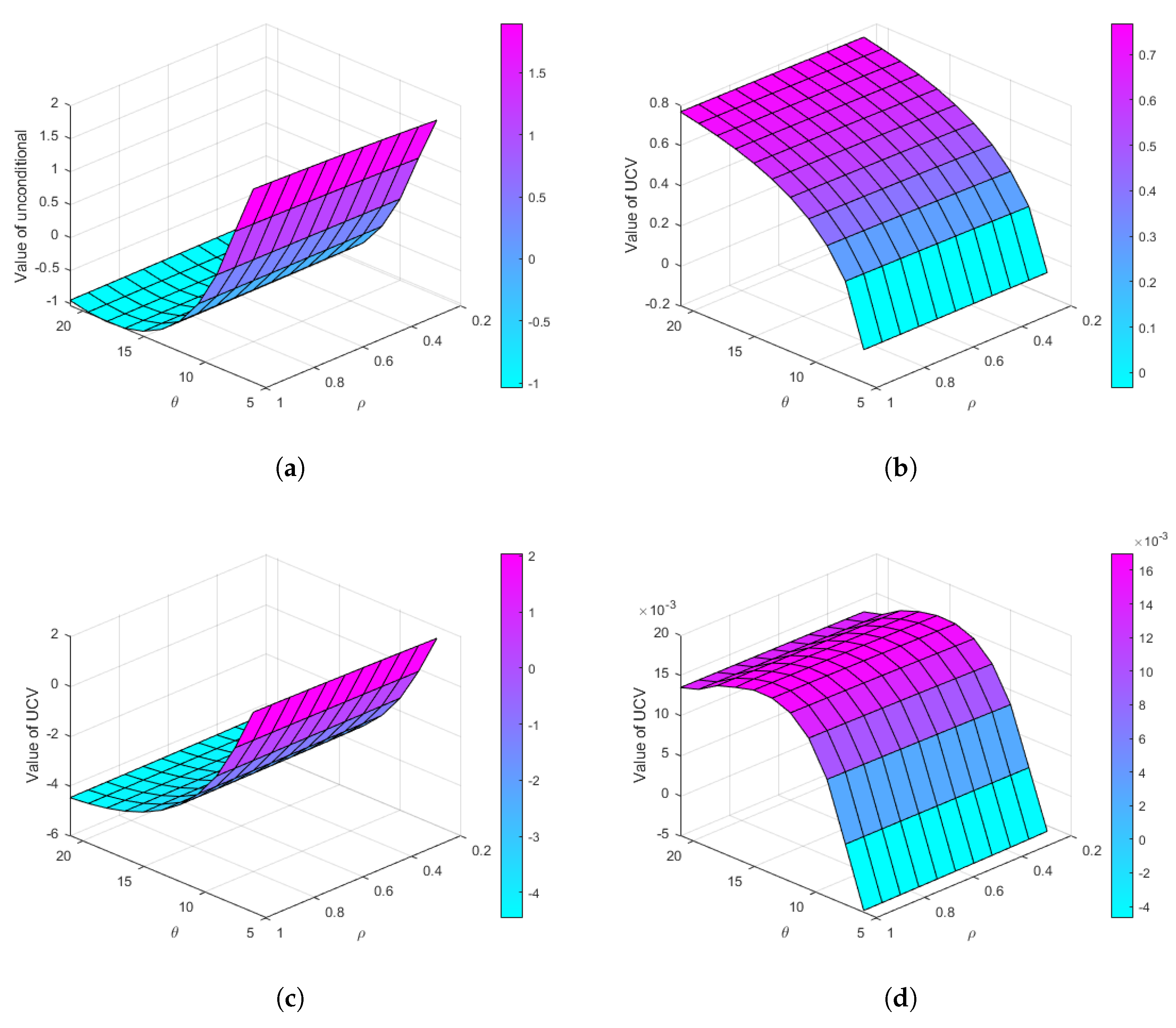
Based on the theory of insufficient effective demand, government fiscal policy is brought to the household utility function and the producer’s production function, thereby influencing household choices and production decisions. Figure 5 shows that when shocked by a positive fiscal spending policy, a sudden increase in government spending in the short run raises aggregate social demand but crowds out private consumption and investment, causing households to increase their labor supply to offset the negative wealth effect of falling consumption. Expansionary policies cause producers to expand production and lower the financing premium by raising inflation through the “Fisher effect”. Thus, producers will hire more labor and rent more capital, leading to higher real rates of return on capital and real wages.
At the same time, the level of carbon emissions increases with output. According to the equilibrium condition for government spending (Equation (44)), expansionary policies require higher carbon taxes as a revenue source, leading to more extraordinary abatement efforts and abatement costs for producers. In the long run, real wages show a positive-to-negative movement caused by the persistent wealth disutility of expansionary policies. On the one hand, while increased government spending can lead to a short-term increase in real wages and a further short-term recovery in household consumption, a prolonged decline in investment leads to the stock of private capital invested in production remaining below its steady-state level, ultimately adversely affecting the productive capacity of society in the long run. On the other hand, the short-run increase in the supply of labor by households may exceed the demand for labor by producers, leading to a downward trend in real wages in the long run due to price stickiness.

5.4.2. Impact of Fiscal Policy Shocks under Low Non-Homothetic Preferences

Non-homothetic preferences also play a financial accelerator in fiscal policy, while the direction remains consistent and the primary transmission mechanism is maintained. The most obvious is that lower elasticities of substitution, non-homothetic parameters and technological efficiency of abatement efforts amplify the impact of shocks on investment, real wages, inflation and price dispersion. Expansionary policies increase the demand for traditional energy products, which has a more significant crowding-out effect on the consumption and investment in traditional energy products by households with a lower preference for low-carbon new energy products.
Also, the shock causes a reallocation of capital and labor from the low-carbon new energy product sector to the traditional energy sector. The fact that the traditional energy sector has some accumulation of capital and labor has resulted in few changes in the real rate of return on capital and labor demand by producers. While the increase in labor supply drives down the marginal returns to labor, the overheating of the economy leads to a more significant increase in the level of inflation. The increase in the general price level leads to a significant decline in real wages, and monetary policy raises nominal interest rates a lot. Lower preferences make carbon tax changes more minor than high preferences, further slowing down producers’ abatement efforts and costs and making it more difficult for governments to achieve carbon emission targets.

5.5. Analysis of the Dynamic Impacts and Transmission Paths of the Mix of Policies

After analyzing the dynamic impact and transmission mechanism of the three major policy shocks, this paper will explores and compare the impacts of different potential mixes of different policies in promoting carbon emission reductions. Since technology shocks are the main driving factors of economic cycle changes, it is essential to study the impact of policy mixes on the economy under technology shocks. This paper argues that a mix of policies is needed to promote the low-carbon process for two reasons. First, in terms of policy targets, policies incorporating a carbon emissions element seek to achieve a certain amount of carbon emissions control at the lowest possible cost within a specific time and spatial horizon. Policies are aimed at receptors, not intermediate objects, and need solutions that make economic development and emission reduction a win–win situation, ensuring that equity and efficiency are achieved together.
However, as different types of policies have different emphases, only a mix of them can bring out their respective advantages so that the “stern hand” of command-and-control policies and the “gentle hand” of “voluntary” economic stimulus policies can be used together to offset the negative impacts and save implementation costs. Second, regarding historical experience and implementation conditions, existing carbon markets in various countries are at the start. At the same time, fiscal and monetary policies have long been utilized and must be coordinated. Thus, this paper sets out that there are two cases in the face of technological shocks. The first is the baseline case in which all three policies include carbon emissions in the policy objective function. The second is in which only two significant policies incorporate carbon emissions into the policy objective function. In contrast, the other policy does not take into account the impact of carbon emissions, resulting in the following three policy mixes, i.e., a mix of carbon price and monetary policy ψ g m = 0 , a mix of carbon price and fiscal policy ψ m = 0 , and a mix of monetary and fiscal policy ψ c e = 0 . This paper assumes that the degree of responsiveness to carbon emissions of the pairwise policy mixes varies year-on-year in response to technology shocks, which also facilitates comparative analysis.

5.5.1. The Impact and Cycle of the Mix of Policies

The results are shown in Figure 6. Under different policy mixes, the main macroeconomic variables move in more or less the same direction. In the baseline case, the supply attributes of the positive technology shock promote an increase in output and carbon emissions in the short run, and there is an increase in consumption and investment but a decline in labor. This results from price stickiness that prevents producers from immediately adjusting their prices in response to an expansion in demand. However, technology shocks allow producers to invest less in factors at a given output level, thus encouraging producers to reduce their labor demand in response to the shock. Rising levels of carbon emissions lead to three policies taking steps to slow the rise in carbon emissions. Carbon pricing policy procyclically increases the carbon tax rate, stimulating producers to increase their abatement efforts, resulting in higher abatement costs to slow the increase in carbon emissions. The primary mechanism by which monetary and fiscal policies reduce carbon emissions is to reduce output. Fiscal policymakers have found that reducing fiscal spending and temporarily reducing household labor supply can mitigate the resource mismatch problem caused by monopolistic competition in the energy products market, thereby reducing the expansion of carbon emissions. Influenced by labor supply and demand, the level of real wages rises.
While monetary policy can reduce the increase in carbon emissions in the long run by raising interest rates, the short-term decline in nominal interest rates and inflation suggests that policymakers have chosen to respond to shocks with accommodative monetary policy, i.e., it is optimal to reduce producer price markups and wage markups, thereby increasing the resources available for consumption and emission reductions in the short run. In the long run, output, the nominal interest rate, the real rate of return on capital, inflation, carbon emissions, abatement costs, abatement efforts and the carbon tax all show opposite responses. The effect of price stickiness will be ignored in the long run. More producers will be able to adjust their prices, and policymakers will no longer have to weigh the cost of abatement against the cost of price adjustment.
In periods 5 to 10, producers are guided by a low-carbon preference to shift to producing new low-carbon energy products. The economy overheats, and monetary policy raises nominal interest rates to curb mild inflation. Real interest rates fall over the period, the real rate of return on capital for producers rises and the carbon tax moves procyclically when paired with monetary policy. Fiscal policy reduces the share of government spending and requires a smaller carbon tax as a source of revenue. As a result, carbon tax changes are gradually reduced, thus causing a decrease in abatement efforts and abatement costs for producers in the long run. The low-carbon new energy products provided by producers in the long term gradually have a dominant market position, forming a locked low-carbon development path. Even if the negative charge of the carbon tax leads to the producers facing fewer abatement efforts and costs, carbon emissions are still reduced to solve the problem of “carbon lock-in”.
Here, this paper considers which policy mix is more effective in reducing carbon emissions when combining three policies in pairs. As can be seen from Figure 6, the mix of carbon price and fiscal policy will cause macroeconomic variables to react strongly when facing technology shocks. The impact of carbon price and monetary policy and the mix of monetary and fiscal policy are relatively the same. At the same time, the differences exist in carbon tax, abatement efforts and abatement costs. The above findings indicate that different policy combinations can have significantly different impacts.
For the carbon price-fiscal policy mix, after a positive technology shock, the carbon price policy raises the carbon tax in response to carbon emissions due to output expansion. Fiscal policy will reduce demand by lowering government spending, and the relevant transmission paths have been discussed above. However, monetary policy does not incorporate carbon emissions into the policy objective function and only needs to focus on inflation and output volatility. Thus, the magnitude of policy adjustment rises significantly. The sticky price leads to a lower real return on capital, and in order to reduce the volatility of credit spreads, monetary policy promptly lowers the nominal interest rate. This pushes the real return on capital back up in the short run, exacerbates capital substitution for labor and increases the dispersion of output and prices. Furthermore, the carbon tax and the capital stock are raised, and government expenditures are reduced, leading to increased volatility of macroeconomic variables relative to the baseline case.
The key to the interaction mechanism between monetary and fiscal policy is that carbon emissions become a common target for both. Governments control carbon emissions mainly by reducing spending, while monetary policy adjusts nominal interest rates to realize its impact on producer financing costs. Monetary policy’s adjustment of nominal interest rates in response to increased carbon emissions affects the effects of fiscal policy, with price stickiness at the beginning of the period leading to a decline in interest rates. Fiscal policy also reduces government spending to reduce carbon emissions, which weakens the extent monetary policy can regulate inflation.
However, the mix is mainly consistent with the impact of the carbon price-monetary policy mix, suggesting that carbon price policy and fiscal policy have some substitution effects when combined with monetary policy. This paper argues that this is because carbon tax revenues under the carbon price policy are a source of fiscal spending. Carbon price policy is no longer responsive to carbon emissions, so the carbon tax does not change in this case. There is no pressure to increase fiscal spending, and a similar carbon price mechanism on the production side of emission reduction is achieved from the aggregate demand side. Instead of the carbon price policy, fiscal policy coordinates with monetary policy to reduce the volatility of carbon emissions due to the increase in aggregate demand. Although the carbon tax does not affect the level of abatement efforts, producers still face positive fluctuations in abatement costs. This is because monetary policymakers use accommodative policies in the short run to lower interest rates and stimulate demand to accommodate output expansion. The opportunity cost of abatement rises for producers. In other words, the monetary-fiscal policy mix does not mitigate the rise in carbon emissions through an autonomous increase in producers’ abatement efforts.

5.5.2. Impact of the Mix of Policies under Low Non-Homothetic Preferences

Furthermore, this paper analyzes the effect of policy mixes when low energy product substitution elasticity and non-homothetic parameters are used to discover the differences caused by non-homothetic preferences. Since this paper wants to examine how economic decision-makers respond to positive technology shocks under lower non-homothetic preferences and given the technological efficiency of abatement efforts, the value assigned to it is not changed here. Figure 7 shows that, in terms of the impact, compared with Figure 6, the magnitude of changes in most economic variables increases under lower elasticity of substitution and non-homothetic parameters. In contrast, investment and labor fluctuations show a shrinking trend. In other words, higher non-homothetic preferences can reduce the impact of policies on macroeconomic variables when responding to positive technology shocks.
Regarding the impact cycle, a lower non-homothetic preference shortens the duration of the impact of technology shocks on economic variables. Regarding the impact of policy mixes, the four policy mixes show different performance from those with high non-homothetic preferences. The impact of the baseline case is no longer in the middle range. However, it substantially impacts output, consumption, nominal interest rates, real capital returns, government spending, carbon emissions, abatement costs, abatement efforts and carbon taxes. The second is the carbon price-monetary policy mix and the monetary-fiscal policy mix. The above three mixes have similar impulse responses when facing technology shocks. However, the carbon price-fiscal policy mix presents different impulse responses, but they are similar to the impulse responses in Figure 6.
Specifically, the lower elasticity of substitution and non-homothetic cases are characterized by insufficient demand for low-carbon energy products. Expansion due to technology shocks satisfy traditional energy demand, and traditional high-carbon production patterns are unconstrained, so the volatility of output and carbon emissions is much higher than in Figure 6. When all three policies target carbon emissions, carbon reduction can only rely on complex policy adjustments because expanding household income does not cause an increase in substitution between energy products. It leads to sharp fluctuations in the economic variables and rapid realization of the steady-state target.
Moreover, reducing non-homothetic preferences promotes households to respond to the impact of the shock with high consumption during the expansionary cycle (since low elasticities imply low price markups). However, the variables quickly converge to the steady state of consumption as the level of inflation returns to a steady state because of policy adjustments. The negative fluctuations in labor supply also return to a steady state in the short run. Technology shocks lead to products being produced at lower prices, and lower relative prices and procyclical changes in investment lead to a short-run increase in the producer’s real rate of return on capital.
When carbon prices are combined with monetary policy, low non-homothetic preferences lead to fiscal policy mitigating the upward pressure on the carbon tax less effectively than in the high-preference case. A decline in the volatility of the carbon tax brings about a decline in the volatility of the other variables. In contrast, in the monetary-fiscal policy mix, the carbon tax is no longer volatile, which brings about a further decline in the volatility of other variables. This suggests that the involvement of carbon price policy is a critical factor in the low-homothetic preference case. As mentioned earlier, a higher carbon tax pressures producers to reduce emissions. However, there is insufficient effective demand for low-carbon energy products, and producers prefer to respond to the pressure to abate through non-low-carbon methods (reducing labor demand and output). As can be seen from the fluctuation of carbon emissions in Figure 7, in the case of a slight difference in the fluctuation of carbon emissions, fluctuation of abatement efforts and abatement costs of producers also show a gradual decrease when the carbon price policy is used in conjunction with the two policies, when it is used in conjunction with the monetary policy and when it is not used, which also proves the above thesis.
Finally, the trend in the volatility of the carbon price-fiscal policy mix is only slightly lower at low preferences, suggesting that this policy mix is less affected by changes in preferences. This is because a rise in the carbon tax for the same change in output makes it necessary for producers to exert abatement efforts regardless of their preferences. In addition, monetary policy only needs to focus on the deviation from output and inflation. It reduces the producer price markup by lowering nominal interest rates and increases consumption in response to rising output. On the other hand, fiscal policy needs to reduce spending to mitigate carbon emissions. The combination of these three effects allows producers to take the same level of mitigation efforts at a high real rate of return on capital under low preferences as they would at a high preference and a low real rate of return on capital, which ultimately makes the impact of this policy mix independent of preferences. This result reflects that a more homogenous source of fiscal revenue in this policy mix can limit the effectiveness of fiscal funds.

6. Welfare Analysis

There are currently two ways of measuring welfare effects: compensating changes and welfare loss functions. Since the welfare loss function is derived from the variance of output and inflation conditional on a particular form of the utility function, it lacks general applicability. Therefore, this paper uses the compensating change in consumption to measure the change in welfare caused by policy implementation to households. It refers to adjustments consumers make in their consumption patterns to offset changes in income or prices, which helps them maintain their overall level of satisfaction or utility despite changes in economic conditions. In addition, ignoring the risk factor for welfare measurement generates large errors. This is because the risk factor included in the higher-order moments (variance measures, i.e., second-order moments) is not taken into account in the first-order approximation [64], the non-stochastic stable state is invariant to the variance of the exogenous shock process. In the second-order approximation, this deterministic equivalence no longer holds, and changes in shock volatility will affect welfare. This is why this paper applies a second-order approximation to the model in the welfare analysis. Finally, although the policy’s short-run impact requires attention, quantifying its long-run welfare effects is essential to policy sustainability. Unconditional consumption compensation is used to measure long-run welfare losses, while conditional consumption compensation assess short-term welfare loss. Considering that the policy’s transition and adjustment costs will disappear in the long run, this paper chooses unconditional consumption compensation to study and define the following unconditional welfare level:
E W e l i A i , K i = E j = 0 β j ln C i , t + j * μ L L i , t + j * 1 + ϕ 1 + ϕ κ ln C E i , t + j *
where i represents before and after policy implementation ( i = B , A ) , C i , t + j * , L i , t + j * , and C E i , t + j * denotes the optimal consumption, labor and carbon emission levels, respectively. According to the property that the effect function is additive and separable, it is defined:
E W e l i C A i , K i E j = 0 β j ln C i , t + j *
E W e l i L A i , K i E j = 0 β j μ L L i , t + j * 1 + ϕ 1 + ϕ
E W e l i C E A i , K i E j = 0 β j κ ln C E i , t + j *
E W e l i A i , K i = E W e l i C A i , K i + E W e l i L A i , K i + E W e l i C E A i , K i
Based on the above form of unconditional welfare, the unconditional consumption compensation change is defined as U C V . It is assumed that after the policy is implemented, U C V units of consumption need to be compensated in order for the welfare level to be the same as before the policy. That is, in order for households to have no difference in welfare before and after policy implementation, the following equation needs to be satisfied:
E W e l B A i , K i = E j = 0 β j ln ( 1 + U C V ) C A , t + j * μ L L A , t + j * 1 + ϕ 1 + ϕ κ ln C E A , t + j *
Substituting the non-homothetic preference utility function and further solving yields the analytic formula for U C V :
U C V = exp ( 1 β ) E W e l B A i , K i E W e l A A i , K i 1
A positive or negative U C V reflects the change in the level of household welfare before and after the implementation of the policy. A positive U C V indicates an increase in household welfare after the implementation of the policy, while a negative U C V indicates a decrease in welfare after the implementation of the policy. A zero U C V indicates no difference in the change in the level of welfare before and after the implementation of the policy.
Unlike other studies, this paper considers the percentage change in consumption compensability before and after the implementation of various cases and policy mixes for all shocks, only carbon price policy shocks, monetary policy shocks, fiscal policy shocks, technology shocks and investment efficiency shocks, respectively, and the results are presented in Table 3. Moreover, this paper shows the change in household welfare at all shocks with different policy mixes and parameter settings in Figure 8. The results in Table 3 show that, from a welfare improvement perspective, the short- and long-term welfare changes under different preferences, shocks and policy mixes do not present the usual DSGE result (i.e., shocks lead to welfare losses and unconditional consumption compensatory changes are always smaller than conditional consumption compensatory changes), but rather exhibit heterogeneous welfare changes. This difference proves that the effects of different carbon-reduction policy portfolios can differ due to different shocks and non-homothetic preferences in the real economic cycle.
For a given type of exogenous shock, the welfare effects resulting from implementing different policy mixes depend on the elasticity of substitution and non-homothetic. Relative to low non-homothetic preferences, at high non-homothetic preferences, the welfare effects of most policy portfolios show a change in direction. For example, implementing the baseline policy mix would shift long-run welfare from a loss of −0.9304% to an improvement of 1.8953% when the full range of shocks is considered, and other policy mixes exhibit the same shift. The same variation as in Table 3 is also shown in Figure 8, indicating that the results in Table 3 are robust. Table 3 shows that in the face of a carbon price policy shock, only the implementation effects of the carbon price-monetary policy mix exhibit a shift from welfare improvement to loss. In the case of a monetary policy shock, all policy mixes exhibit a shift in the direction of long-run welfare. In the case of a fiscal policy shock, the long-run welfare after implementing the policy mixes, except for the carbon price-monetary policy, exhibits a shift in direction. In the case of a technology shock, only the carbon price-monetary policy portfolios shift their long-run welfare effects. In the case of investment shocks, the welfare effects before and after the implementation of policy portfolios are not affected by non-homothetic preferences.
To summarize: (i) In the presence of positive fiscal and monetary policy shocks, higher non-non-homothetic preferences make it likely that the carbon price-fiscal policy mix will improve welfare when curbing carbon emissions. The reason is that the high non-homothetic preference setting reflects the household’s preference for low carbon and the positive utility-enhancing effect of emission reduction in the utility function. As discussed earlier, a fiscal shock requires a higher level of carbon tax as a source of revenue. The carbon tax is thus unexpectedly raised, and producers’ level of abatement efforts responds to this, gradually transmitting to an abatement behavior. Similarly, an unexpected rise in nominal interest rates reduces carbon emissions from production while discouraging consumption and investment. It is worth noting that policymakers need to respond to lower inflation regardless of whether the monetary policy function considers carbon emissions. The “Fisher effect” of expansionary fiscal policy indirectly restores inflation to its steady-state level from a fiscal perspective, reducing the efficiency loss in the policy implementation process. On the contrary, with low non-homothetic preferences, households are more reluctant to substitute consumption across periods. They cannot substitute consumption with periods of higher marginal utility of consumption and prefer traditional energy products. Positive fiscal and monetary policy shocks lead to a tighter carbon price, fiscal and monetary policy, resulting in negative utility from short-run increases in carbon emissions from reduced household consumption and expansionary shocks, ultimately resulting in a loss of long-run welfare. (ii) This paper also finds that under low preferences, monetary policy increases the level of welfare when paired with a carbon price and fiscal policy that includes an emission-reduction target, respectively. Any positive shock will raise the carbon tax and the nominal interest rate, thereby mitigating carbon emissions. The central bank lowers the nominal interest rate according to the monetary rule in response to the shocks. Since households’ low preferences will not lead them to substitute across time, this will encourage them to consume more, thus increasing the welfare level. In contrast, the pairing between a carbon price and fiscal policy is a powerful channel for abatement, inducing traditional energy consumption by households with low non-homothetic preferences, which results in a long-run welfare loss.
Table 3 shows that the relative magnitude of long- and short-run welfare effects before and after policy implementation is not perfectly uniform and still shifts with non-homothetic preferences. Specifically, the short-run welfare improvement of the carbon price-monetary policy mix and the monetary-fiscal policy mix at low preferences is higher than the long-run welfare improvement when there is only a monetary shock. Although welfare is lost when there is a high preference, the long-run welfare loss is lower than the short-run welfare loss. Similarly, the post-implementation welfare improvement (loss) of a policy mix that includes a carbon price under high preferences when faced with the carbon price and technology shocks is significantly higher (lower) than the welfare situation in the low-preference case. That is, the policy implementation is more attractive to high-preference households. This finding suggests that an increase in non-homothetic preferences may be the critical mechanism by which post-policy implementation shocks increase long-run welfare or dampen welfare loss in the long run. So, what is this crucial mechanism? According to the First Fundamental Theorem of Welfare Economics, every Walrasian equilibrium allocation is Pareto efficient, so it is natural to assume that fluctuations after policy implementation always reduce welfare. However, the increase in non-homothetic preferences increases the substitutability between low-carbon new and traditional energy products. Producers will respond to higher demand by increasing new, low-carbon energy products. The increase in the quantity of products produced also reduces the price of the relevant products in the long run. The decline in the price index tends to increase the real wage further, creating a mechanism of intertemporal substitution. Carbon price shocks, monetary policy shocks and technology shocks are exogenous fluctuations closely related to the production side of the equation. The unexpected positive shocks will induce households to provide more labor and take advantage of higher real wages and lower price expectations to consume more in the future. The shocks anticipate the long-term goal of the “dual carbon” policy, and the variables above change through the intertemporal substitution mechanism of high preferences. In this case, increasing non-homothetic preferences imparts an “option”-like property to low-carbon production. A mix including carbon price policies is used to face the three shocks. The greater the shock volatility, the more valuable the “option” will be, and household welfare will improve or lose less in the long run.
From the differences between unconditional and conditional consumption compensation in Table 3, the differences between the baseline case and the long and short run of the carbon price-fiscal policy mix decrease at high levels of preferences, while the differences between the other two policy mixes increase. This result suggests that high non-homothetic preferences make the former case have a minor impact on the average capital stock in the face of shocks compared to the latter. The reason is that the mix containing a carbon price and fiscal policy enhances the ability of high-preference households to utilize shocks for intertemporal substitution. In contrast, the remaining policy mixes do not. This paper introduces capital stock utilization into the model, which makes capital elastic in the short run, increases the overall factor supply elasticity and amplifies the change in welfare due to the shock. The former case works because of the coordination between policies. That is, carbon pricing policies affect monetary and fiscal policies while targeting producer carbon emissions, fiscal policy affects carbon prices and monetary policy while targeting aggregate social demand and monetary policy targets carbon emissions and inflation while influencing carbon price and fiscal policy. Among them, the match of carbon price and fiscal policy plays an important role. Carbon tax is the source of fiscal expenditure, and carbon price policy leads to synchronized changes in fiscal policy. Under the standard emission-reduction target, one can take action. At the same time, the other can choose a discretionary way, reducing the cost of proactive adjustments. At the same time, high-preference households are able to make quick intertemporal adjustments to reduce the average capital loss in the short-run policies. Finally, the average capital stock increases as shocks increase, and high preferences endow this policy mix with more capital in the face of shocks than in low preference cases.

7. Conclusions and Policy Implications

How can the carbon market, as a significant tool, facilitate the achievement of carbon emission-reduction targets in a twin-track way with economic development? Is there an interaction between macroeconomic policies and carbon markets? What is different from the past is that carbon pricing behavior caused by the carbon market will affect the implementation effect of policy mixes and changes in household welfare, and this impact will vary depending on non-homothetic preferences. Based on the above reality, this paper, based on the supply side and demand side, constructs an environmental dynamic stochastic general equilibrium model of six departments, including households, intermediate and final product producers, carbon market, central bank and government with non-homothetic consumption preferences. This paper analyzes economic effects, transmission mechanisms and welfare effects under different exogenous shocks, policy mixes and non-homothetic preferences. This paper draws the following main conclusions through policy simulation analysis.
First, coordinating carbon markets and macroeconomic policies can simultaneously achieve economic and environmental goals. When a positive carbon price shock impacts the policy, it reduces emissions. The existence of price stickiness means that abatement does not need to be maintained for a long time. Meanwhile, the supply capacity and output level will be improved due to the demand-pull of non-homothetic preferences, further increasing labor and real wages.
Second, when monetary policy incorporating carbon emission targets faces positive external shocks, it suppresses carbon emissions through the interest rate channel by suppressing demand and reducing output. Fiscal policy works similarly, which uses fiscal expenditures to affect total social demand and regulate carbon emission levels.
Third, when considering non-homothetic preferences, higher non-homothetic preferences will expand the economic cycle fluctuations caused by exogenous shocks and act as a “financial accelerator” for the transmission path of policies.
Fourth, it is further found that the mix of policies promoting carbon emission reduction will produce heterogeneous effects under the influence of non-homothetic preferences. Also, higher non-homothetic preferences can lead to a reduction in the magnitude and lengthening of the period of policy influence on macroeconomic variables compared to low non-homothetic preferences. Moreover, the “carbon lock-in” problem can be solved in the long run when the three policies are implemented together.
Fifth, welfare analysis suggests that differences in the relative size and variance of the welfare effects, long- and short-term effects, resulting from implementing different policy mixes, depend on the level of non-homothetic preferences. The intertemporal substitution mechanism with high non-homothetic preferences imparts an “option”-like character to low-carbon production. The findings of this paper are of great significance for expanding the field of carbon market research and comprehensively recognizing the emission-reduction effects of the government’s “macroeconomic policy package”. This paper obtains the following policy implications.
First, promote synergistic development of the carbon market and economy and society. Carbon markets can support productivity and innovation in low-carbon new energy products and sustainable industries through price signals, creating more jobs. Also, carbon markets can encourage financial investment in low-carbon, net-zero and net-negative technologies and support additional economic incentives and investment programs.
Second, clarify the monetary policy mix’s role in climate regulation. The pairing of monetary policy and carbon market construction can improve liquidity, promote capital accumulation and changes in the rate of return on capital and guide the transfer of capital elements to the new energy industry. However, it is necessary to guard against systemic financial risks.
Third, build a comprehensive, integrated and linked environmental fiscal policy system. Current green fiscal policies rely heavily on carbon tax revenues, but a single source of fiscal revenue for carbon emissions management can limit the regulatory effect of fiscal policy. Therefore, a sound-linked financial system should be constructed to recover quickly from shocks.
Fourth, advocate vigorously for green and low-carbon public consumption. In the face of technology shocks, increasing green consumption preferences can mitigate the magnitude of economic changes and reduce the costs of short-term policy adjustments. The government should stimulate a preference for more renewable energy, and ensure economic stability and decarbonization of development.
Fifth, enhance systemic thinking and risk prevention in carbon-reduction policies. In formulating these policies, the government must fully consider the spillover effects between them, strengthen their systemic and synergistic nature, and avoid conflicts and superposition of policies with the same goals.

Author Contributions

Conceptualization, X.D. and G.M.; methodology, X.D. and G.M.; software, X.D.; formal analysis, X.D. and G.M.; data curation, X.D. and G.M.; writing—original draft preparation, X.D. and G.M.; writing—review and editing, X.D., G.M. and J.C.; supervision, G.M. and J.C.; funding acquisition, G.M. and J.C.; Investigation, X.D. and J.C.; visualization, X.D., G.M. and J.C.; All authors have read and agreed to the published version of the manuscript.

Funding

This research was funded by Shanghai Social Science Planning Annual Project grant number 2021BJB003 and the Fundamental Research Funds for the Central Universities CXJJ-2023-430. The APC was funded by Shanghai Social Science Planning Annual Project.

Institutional Review Board Statement

Not applicable.

Informed Consent Statement

Not applicable.

Data Availability Statement

The original contributions presented in the study are included in the article, further inquiries can be directed to the corresponding author.

Acknowledgments

The authors sincerely thank the reviewers for their helpful comments and suggestions about our manuscript.

Conflicts of Interest

The authors declare no conflicts of interest.

References

  1. World Bank. State and Trends of Carbon Pricing 2021; The World Bank: Washington, DC, USA, 2021. [Google Scholar] [CrossRef]
  2. Lightfoot, S.; Burchell, J. Green hope or greenwash? The actions of the European Union at the World Summit on sustainable development. Glob. Environ. Chang. 2004, 14, 337–344. [Google Scholar] [CrossRef]
  3. Honma, S.; Ushifusa, Y.; Okamura, S.; Vandercamme, L. Measuring carbon emissions performance of Japan’s metal industry: Energy inputs, agglomeration, and the potential for green recovery reduction. Resour. Policy 2023, 82, 103519. [Google Scholar] [CrossRef]
  4. Yu, D.J.; Li, J. Evaluating the employment effect of China’s carbon emission trading policy: Based on the perspective of spatial spillover. J. Clean. Prod. 2021, 292, 126052. [Google Scholar] [CrossRef]
  5. Waleed, K.; Mirza, F.M. Examining behavioral patterns in household fuel consumption using two-stage-budgeting framework for energy and environmental policies: Evidence based on micro data from Pakistan. Energy Policy 2020, 147, 111835. [Google Scholar] [CrossRef]
  6. Li, R.; Leung, G.C. The relationship between energy prices, economic growth and renewable energy consumption: Evidence from Europe. Energy Rep. 2021, 7, 1712–1719. [Google Scholar] [CrossRef]
  7. Tovar Reaños, M.A.; Lynch, M.A. Measuring carbon tax incidence using a fully flexible demand system. Vertical and horizontal effects using Irish data. Energy Policy 2022, 160, 112682. [Google Scholar] [CrossRef]
  8. Cavallari, L.; Etro, F. Demand, markups and the business cycle. Eur. Econ. Rev. 2020, 127, 103471. [Google Scholar] [CrossRef]
  9. Liu, J.; Gong, N.; Qin, J. How would the carbon tax on energy commodities affect consumer welfare? Evidence from China’s household energy consumption system. J. Environ. Manag. 2022, 317, 115466. [Google Scholar] [CrossRef] [PubMed]
  10. Galeotti, M.; Lanza, A. Desperately seeking environmental Kuznets. Environ. Model. Softw. 2005, 20, 1379–1388. [Google Scholar] [CrossRef]
  11. Ma, G.; Qin, J.; Zhang, Y. Does the carbon emission trading system reduce carbon emissions by promoting two-way FDI in developing countries? Evidence from Chinese listed companies and cities. Energy Econ. 2023, 120, 106581. [Google Scholar] [CrossRef]
  12. Bartocci, A.; Notarpietro, A.; Pisani, M. “Green” fiscal policy measures and nonstandard monetary policy in the euro area. Econ. Model. 2024, 136, 106743. [Google Scholar] [CrossRef]
  13. Gelfer, S. Examining business cycles and optimal monetary policy in a regional DSGE model. Econ. Model. 2024, 136, 106750. [Google Scholar] [CrossRef]
  14. Annicchiarico, B.; Dio, F.D. GHG Emissions Control and Monetary Policy. Environ. Resour. Econ. 2017, 67, 823–851. [Google Scholar] [CrossRef]
  15. Borenstein, S.; Bushnell, J.; Wolak, F.A.; Zaragoza-Watkins, M. Expecting the Unexpected: Emissions Uncertainty and Environmental Market Design. Am. Econ. Rev. 2019, 109, 3953–3977. [Google Scholar] [CrossRef]
  16. Rozenberg, J.; Vogt-Schilb, A.; Hallegatte, S. Instrument choice and stranded assets in the transition to clean capital. J. Environ. Econ. Manag. 2020, 100, 102183. [Google Scholar] [CrossRef]
  17. Sun, J.; Wang, F.; Yin, H.; Zhang, B. Money Talks: The Environmental Impact of China’s Green Credit Policy. J. Policy Anal. Manag. 2019, 38, 653–680. [Google Scholar] [CrossRef]
  18. Blazquez, J.; Galeotti, M.; Manzano, B.; Pierru, A.; Pradhan, S. Effects of Saudi Arabia’s economic reforms: Insights from a DSGE model. Econ. Model. 2021, 95, 145–169. [Google Scholar] [CrossRef]
  19. Hou, R.; Lei, L.; Jin, K.; Lin, X.; Xiao, L. Introducing electric vehicles? Impact of network effect on profits and social welfare. Energy 2022, 243, 123002. [Google Scholar] [CrossRef]
  20. Matsumura, K.; Naka, T.; Sudo, N. Analysis of the transmission of carbon taxes using a multi-sector DSGE. Energy Econ. 2024, 136, 107642. [Google Scholar] [CrossRef]
  21. Garcia-Villegas, S.; Martorell, E. Climate transition risk and the role of bank capital requirements. Econ. Model. 2024, 135, 106724. [Google Scholar] [CrossRef]
  22. Crocker, T. The Structuring of Atmospheric Pollution Control Systems. Econ. Air Pollut. 1966, 61, 81–84. [Google Scholar] [CrossRef]
  23. Bel, G.; Joseph, S. Emission abatement: Untangling the impacts of the EU ETS and the economic crisis. Energy Econ. 2015, 49, 531–539. [Google Scholar] [CrossRef]
  24. Schäfer, S. Decoupling the EU ETS from subsidized renewables and other demand side effects: Lessons from the impact of the EU ETS on CO2 emissions in the German electricity sector. Energy Policy 2019, 133, 110858. [Google Scholar] [CrossRef]
  25. Liu, Y.; Tan, X.J.; Yu, Y.; Qi, S.Z. Assessment of impacts of Hubei Pilot emission trading schemes in China—A CGE-analysis using TermCO2 model. Appl. Energy 2017, 189, 762–769. [Google Scholar] [CrossRef]
  26. Yu, Y.; Zhang, W.; Zhang, N. The Potential Gains from Carbon Emission Trading in China’s Industrial Sectors. Comput. Econ. 2018, 52, 1175–1194. [Google Scholar] [CrossRef]
  27. Zhang, Y.; Li, S.; Luo, T.; Gao, J. The effect of emission trading policy on carbon emission reduction: Evidence from an integrated study of pilot regions in China. J. Clean. Prod. 2020, 265, 121843. [Google Scholar] [CrossRef]
  28. Li, R.; Ramanathan, R. Exploring the relationships between different types of environmental regulations and environmental performance: Evidence from China. J. Clean. Prod. 2018, 196, 1329–1340. [Google Scholar] [CrossRef]
  29. Zhao, J.; Jiang, Q.; Dong, X.; Dong, K. Would environmental regulation improve the greenhouse gas benefits of natural gas use? A Chinese case study. Energy Econ. 2020, 87, 104712. [Google Scholar] [CrossRef]
  30. Du, Z.; Xu, C.; Lin, B. Does the Emission Trading Scheme achieve the dual dividend of reducing pollution and improving energy efficiency? Micro evidence from China. J. Environ. Manag. 2022, 323, 116202. [Google Scholar] [CrossRef]
  31. Tan, X.; Liu, Y.; Cui, J.; Su, B. Assessment of carbon leakage by channels: An approach combining CGE model and decomposition analysis. Energy Econ. 2018, 74, 535–545. [Google Scholar] [CrossRef]
  32. Wen, F.; Wu, N.; Gong, X. China’s carbon emission trading and stock returns. Energy Econ. 2020, 86, 104627. [Google Scholar] [CrossRef]
  33. Cui, L.B.; Fan, Y.; Zhu, L.; Bi, Q.H. How will the emission trading scheme save cost for achieving China’s 2020 carbon intensity reduction target? Appl. Energy 2014, 136, 1043–1052. [Google Scholar] [CrossRef]
  34. Wesseh, P.K.; Lin, B. Optimal carbon taxes for China and implications for power generation, welfare, and the environment. Energy Policy 2018, 118, 1–8. [Google Scholar] [CrossRef]
  35. Geng, W.; Fan, Y. Emission trading in an imperfectly competitive product market: A comparison of social welfare under mass- and rate-based schemes. Comput. Ind. Eng. 2021, 162, 107761. [Google Scholar] [CrossRef]
  36. Mayer, J.; Dugan, A.; Bachner, G.; Steininger, K.W. Is carbon pricing regressive? Insights from a recursive-dynamic CGE analysis with heterogeneous households for Austria. Energy Econ. 2021, 104, 105661. [Google Scholar] [CrossRef]
  37. Heutel, G. How should environmental policy respond to business cycles? Optimal policy under persistent productivity shocks. Rev. Econ. Dyn. 2012, 15, 244–264. [Google Scholar] [CrossRef]
  38. Fischer, C.; Springborn, M. Emissions targets and the real business cycle: Intensity targets versus caps or taxes. J. Environ. Econ. Manag. 2011, 62, 352–366. [Google Scholar] [CrossRef]
  39. Annicchiarico, B.; Di Dio, F. Environmental policy and macroeconomic dynamics in a new Keynesian model. J. Environ. Econ. Manag. 2015, 69, 1–21. [Google Scholar] [CrossRef]
  40. Dissou, Y.; Karnizova, L. Emissions cap or emissions tax? A multi-sector business cycle analysis. J. Environ. Econ. Manag. 2016, 79, 169–188. [Google Scholar] [CrossRef]
  41. Katircioglu, S.; Katircioglu, S. Testing the role of fiscal policy in the environmental degradation: The case of Turkey. Environ. Sci. Pollut. Res. 2018, 25, 5616–5630. [Google Scholar] [CrossRef]
  42. Economides, G.; Xepapadeas, A. Monetary Policy under Climate Change; CESifo Working Paper 7021; Munich Society for the Promotion of Economic Research-CESifo GmbH: Munich, Germany, 2018. [Google Scholar]
  43. Jacobs, B.W.; Singhal, V.R.; Subramanian, R. An empirical investigation of environmental performance and the market value of the firm. J. Oper. Manag. 2010, 28, 430–441. [Google Scholar] [CrossRef]
  44. Kumar, A.; Jain, V.; Kumar, S. A comprehensive environment friendly approach for supplier selection. Omega 2014, 42, 109–123. [Google Scholar] [CrossRef]
  45. Ji, J.; Zhang, Z.; Yang, L. Carbon emission reduction decisions in the retail-/dual-channel supply chain with consumers’ preference. J. Clean. Prod. 2017, 141, 852–867. [Google Scholar] [CrossRef]
  46. Xia, L.; Hao, W.; Qin, J.; Ji, F.; Yue, X. Carbon emission reduction and promotion policies considering social preferences and consumers’ low-carbon awareness in the cap-and-trade system. J. Clean. Prod. 2018, 195, 1105–1124. [Google Scholar] [CrossRef]
  47. Wang, Y.; Wang, F. Production and emission reduction decisions considering the differentiated carbon tax regulation across new and remanufactured products and consumer preference. Urban Clim. 2021, 40, 100992. [Google Scholar] [CrossRef]
  48. Dogan, E.; Muhammad, I. Willingness to pay for renewable electricity: A contingent valuation study in Turkey. Electr. J. 2019, 32, 106677. [Google Scholar] [CrossRef]
  49. Ndebele, T. Assessing the potential for consumer-driven renewable energy development in deregulated electricity markets dominated by renewables. Energy Policy 2020, 136, 111057. [Google Scholar] [CrossRef]
  50. Liobikienė, G.; Dagiliūtė, R. Do positive aspects of renewable energy contribute to the willingness to pay more for green energy? Energy 2021, 231, 120817. [Google Scholar] [CrossRef]
  51. Cardella, E.; Ewing, B.T.; Williams, R.B. Green is Good—The Impact of Information Nudges on the Selection of Voluntary Green-Power Plans. Energy J. 2022, 43, 1–42. [Google Scholar] [CrossRef]
  52. Sun, C.; Wang, Y.; Zhu, Z.; Qiu, L. Decoupling carbon emissions from the economy and low-carbon ecological city construction-based on 196 cities in China. Sustain. Cities Soc. 2024, 107, 105458. [Google Scholar] [CrossRef]
  53. Bertoletti, P.; Etro, F. Monopolistic Competition when Income Matters. Econ. J. 2017, 127, 1217–1243. [Google Scholar] [CrossRef]
  54. Erceg, C.; Henderson, D.; Levin, A. Optimal Monetary Policy With Staggered Wage and Price Contracts. J. Monet. Econ. 2000, 46, 281–313. [Google Scholar] [CrossRef]
  55. Calvo, G.A. Staggered prices in a utility-maximizing framework. J. Monet. Econ. 1983, 12, 383–398. [Google Scholar] [CrossRef]
  56. Gourio, F. Disaster Risk and Business Cycles. Am. Econ. Rev. 2012, 102, 2734–2766. [Google Scholar] [CrossRef]
  57. Christiano, L.J.; Trabandt, M.; Walentin, K. Chapter 7–DSGE Models for Monetary Policy Analysis. In Handbook of Monetary Economics; Elsvier: Amsterdam, The Netherlands, 2010; Volume 3, pp. 285–367. [Google Scholar] [CrossRef]
  58. Zhang, J.; Zhang, Y. Examining the economic and environmental effects of emissions policies in China: A Bayesian DSGE model. J. Clean. Prod. 2020, 266, 122026. [Google Scholar] [CrossRef]
  59. Annicchiarico, B.; Diluiso, F. International transmission of the business cycle and environmental policy. Resour. Energy Econ. 2019, 58, 101112. [Google Scholar] [CrossRef]
  60. Pan, X.; Xu, H.; Li, M.; Zong, T.; Lee, C.T.; Lu, Y. Environmental expenditure spillovers: Evidence from an estimated multi-area DSGE model. Energy Econ. 2020, 86, 104645. [Google Scholar] [CrossRef]
  61. Xiao, B.; Fan, Y.; Guo, X.; Voigt, S.; Cui, L. Effects of linking national carbon markets on international macroeconomics: An open-economy E-DSGE model. Comput. Ind. Eng. 2022, 169, 108166. [Google Scholar] [CrossRef]
  62. Chan, Y.T. Are macroeconomic policies better in curbing air pollution than environmental policies? A DSGE approach with carbon-dependent fiscal and monetary policies. Energy Policy 2020, 141, 111454. [Google Scholar] [CrossRef]
  63. Noureen, S.; Iqbal, J.; Chishti, M. Exploring the dynamic effects of shocks in monetary and fiscal policies on the environment of developing economies: Evidence from the CS-ARDL approach. Environ. Sci. Pollut. Res. 2022, 29, 45665–45682. [Google Scholar] [CrossRef]
  64. Schmitt-Grohé, S.; Uribe, M. Solving dynamic general equilibrium models using a second-order approximation to the policy function. J. Econ. Dyn. Control. 2004, 28, 755–775. [Google Scholar] [CrossRef]
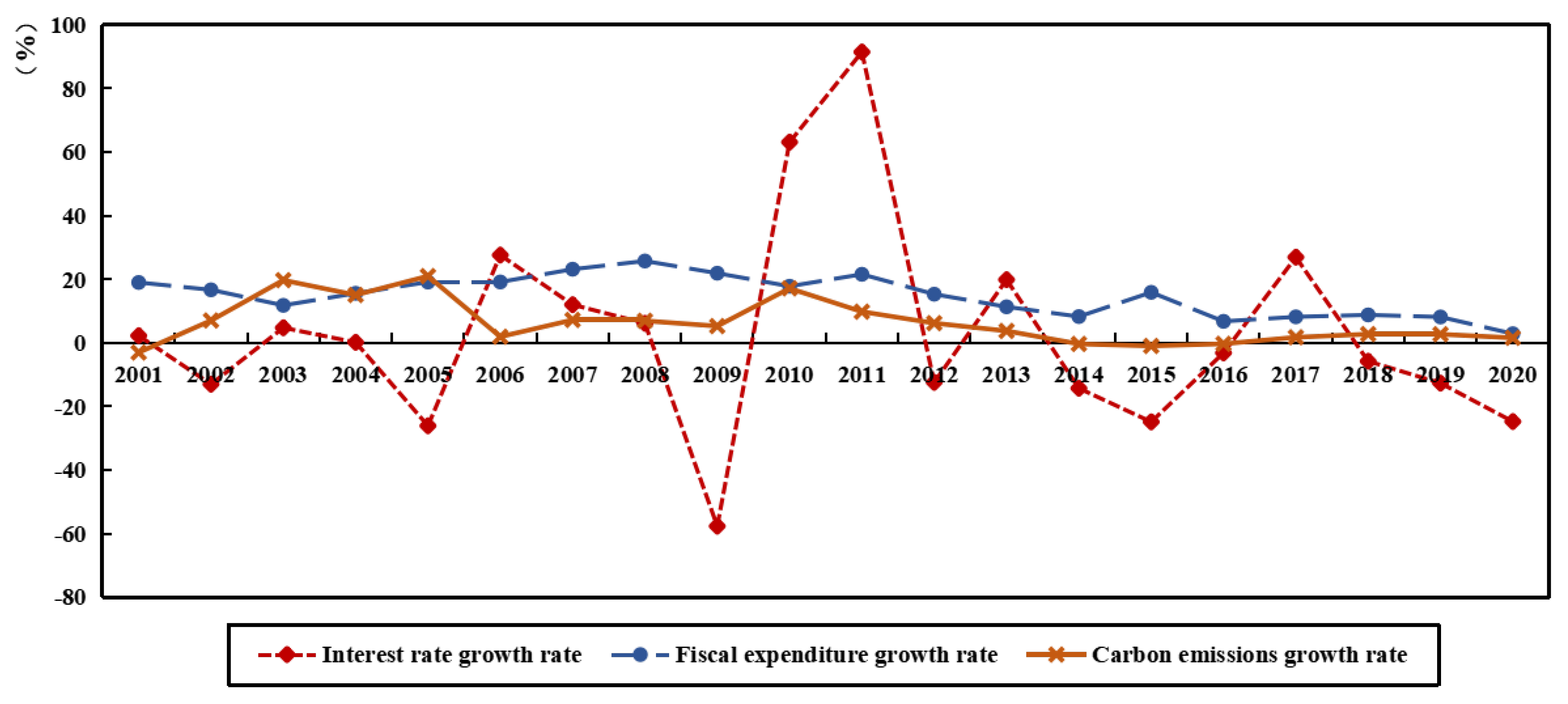
Figure 1. China’s interest rate, fiscal expenditure and carbon emission growth rate from 2001 to 2020.
Sustainability 16 06741 g001
Figure 2. Impulse responses of carbon price policy shocks to major economic variables.
Sustainability 16 06741 g002
Figure 3. Impulse responses of COVID-19 shocks to major economic variables.
Sustainability 16 06741 g003
Figure 4. Impulse responses of monetary policy shocks to major economic variables.
Sustainability 16 06741 g004
Figure 5. Impulse responses of fiscal policy shocks to major economic variables.
Sustainability 16 06741 g005
Figure 6. Impulse responses of technology shocks to major economic variables in different policy mixes.
Sustainability 16 06741 g006
Figure 7. Impulse responses of technology shocks to major economic variables in different policy mixes with low elasticity of substitution and non-homothetic.
Sustainability 16 06741 g007
Figure 8. Changes in household welfare under full shocks with different policy mixes and parameter settings. (a) Unconditional consumption compensation for households in the baseline case. (b) Unconditional consumption compensation for households with carbon price policy & monetary policy. (c) Unconditional consumption compensation for households with carbon price policy & fiscal policy. (d) Unconditional consumption compensation for households with monetary policy & fiscal policy.
Sustainability 16 06741 g008
Table 1. The result of calibration.
ParameterDescriptionValueLiterature Backed
β Discount factor0.9904Chan [62]
μ L Parameter of labor disutilityCalculated by steady-state
ϕ Inverse of Frisch elasticity1.0000Christiano et al. [57]
κ Parameter of emissions disutility0.2000Zhang and Zhang [58]
δ K Depreciation rate of capital0.0250Chan [62]
γ I Parameter of price adjustment cost2.0000Pan et al. [60], Xiao et al. [61]
λ 1 Parameter of capital utilization costCalculated by steady-state
λ 2 Parameter of capital utilization cost0.0100Christiano et al. [57]
θ Elasticity of substitution of energy products6.0000Annicchiarico and Diluiso [59]
ρ Parameter of non-homothetic1.0000Bertoletti and Etro [53]
Φ w Parameter of wage stickiness0.7500Calvo [55]
ε Elasticity of substitution of labor supply6.0000Chan [62]
α Share of capital in production 1 / 3 Annicchiarico and Diluiso [59]
γ ( C E ) Damage parameter of carbon emissions0.0026Heutel [37]
χ Technological efficiency parameter of abatement efforts0.4500Annicchiarico and Dio [14]
ϕ 1 Scale parameter of controlling abatement costs0.1850Annicchiarico and Dio [14]
ϕ 2 Elasticity of abatement costs to abatement efforts2.8000Annicchiarico and Dio [14]
τ p ¯ Steady-state carbon price in carbon markets0.0500Chan [62]
G E ¯ Steady-state share of government expenditures0.2000Chan [62]
Φ p Parameter of price stickiness0.7500Calvo [55]
Table 2. The Bayes estimation of parameters.
ParameterPrior DistributionPosterior Distribution
Prior DistPrior MeanPrior SDPosterior Mean90% Confidence Interval
ψ τ Beta0.50000.10000.4032 [ 0.3969 , 0.4096 ]
ψ c e Normal1.50000.10001.7460 [ 1.7439 , 1.7481 ]
ψ r Beta0.50000.20000.1458 [ 0.1414 , 0.1501 ]
ψ π Normal1.60000.10001.5643 [ 1.5642 , 1.5645 ]
ψ Y Normal0.10000.05000.4088 [ 0.4075 , 0.4101 ]
ψ m Normal0.12000.20000.0851 [ 0.0849 , 0.0854 ]
ψ g Beta0.50000.20000.9569 [ 0.9547 , 0.9590 ]
ψ g m Normal0.05000.02000.0443 [ 0.0434 , 0.0452 ]
ρ Z Beta0.70000.20000.7721 [ 0.7707 , 0.7735 ]
ρ A Beta0.70000.20000.9883 [ 0.9775 , 0.9991 ]
ρ C O V Beta0.50000.02000.5328 [ 0.5326 , 0.5331 ]
Table 3. Welfare analysis of policies under different circumstances.
ShockNon-Homotheticity
θ = 6 , ρ = 1 θ = 21 , ρ = 0 . 25
Policy MixPolicy Mix
BaselineC + FC + MM + FBaselineC + FC + MM + F
All Shocks1.8952.046−0.034−0.004−0.930−4.3890.7570.013
(3.597)(4.502)(−0.090)(−0.012)(0.894)(−1.486)(0.711)(0.003)
Carbon price−0.246−0.036−0.1790.364−3.757−7.3140.7740.014
(−0.593)(−0.160)(−0.360)(0.867)(−3.757)(−7.314)(0.774)(0.014)
Monetary2.1592.346−0.031−0.015−0.922−4.3780.7460.004
(3.672)(4.527)(−0.074)(−0.029)(0.560)(−1.984)(0.715)(−0.005)
Fiscal0.0020.0080.006−0.053−3.755−7.3140.7740.014
(0.009)(0.001)(0.001)(−0.116)(−3.752)(−7.314)(0.775)(0.014)
Technology−0.026−0.016−0.0080.001−3.696−7.2410.7710.014
(−0.050)(−0.028)(−0.017)(0.002)(−3.663)(−7.191)(0.768)(0.014)
Investment−0.234−0.2770.0050.010−3.828−7.3980.7860.022
(−0.025)(0.004)(0.005)(0.014)(−3.536)(−6.967)(0.774)(0.022)
Disclaimer/Publisher’s Note: The statements, opinions and data contained in all publications are solely those of the individual author(s) and contributor(s) and not of MDPI and/or the editor(s). MDPI and/or the editor(s) disclaim responsibility for any injury to people or property resulting from any ideas, methods, instructions or products referred to in the content.