The Impacts of Regulatory Approaches to Carbon Quotas on Third-Party Logistics Low-Carbon Financing Strategies and Emission Reduction Effects

Abstract

Carbon emission reduction is an important issue for sustainable development. The logistics industry is a key area for carbon emission reduction. The modern logistics supply chain includes logistics parks (fourth-party logistics, 4PL) and small, medium and micro logistics enterprises settled in the parks (third-party logistics, 3PL). Facing the pressure of the need for sustainable development, 3PL enterprises need to invest a lot of money in green transformation. However, 3PL enterprises are subject to serious financial constraints. In order to break the capital constraints, 3PL enterprises can raise funds from banks or from 4PL financing. Under the carbon quota policy, the government can regulate the 4PL or the 3PL. Therefore, this paper uses the Stackelberg game model to build a green financing strategy model of small and medium-sized logistics enterprises considering different supervision methods under carbon quotas, explores the optimal emission reduction decision-making process of small and medium-sized logistics enterprises, and provides solutions to the financing problems of small and medium-sized logistics enterprises in realizing sustainable development. The study found that the decisions of enterprises under different governmental supervision methods are affected by carbon quotas, and the government’s supervision of 3PL is more conducive to carbon emission reduction; in this scenario, the 4PL financing strategy is more likely to be adopted compared with bank financing, because 4PL charge lower service fees, thus encouraging 3PL to increase their low-carbon investment. Finally, this paper puts forward two different carbon emission supervision methods and considers the green financing services of 4PL; this provides references for government supervision and the sustainable development strategies of logistics enterprises.

1. Introduction

With the increasingly serious global climate problem, carbon emissions have become a stumbling block to environmentally sustainable development; people are deeply aware that reducing greenhouse gas emissions and curbing climate change is the only way to achieve sustainable development. Therefore, governments of all countries are actively responding to the theme of “green and low-carbon”, taking measures to control and reduce greenhouse gas emissions, among which the control and supervision of carbon emissions of enterprises has become one of the effective measures to reduce greenhouse gas emissions. With the proposal of China’s “dual carbo goals”, new requirements have been put forward for carbon emissions of various industries. At present, China is gradually establishing a carbon market and promoting the idea that enterprises should reduce carbon emissions through the formulation of carbon emission standards, the implementation of a carbon tax and carbon trading. Seven provinces and cities, including Beijing, Shanghai, Hubei and Shenzhen, have been piloting carbon trading to encourage enterprises to reduce carbon emissions by limiting their carbon emissions in the form of quantitative carbon emission allowances allocated by the government. At the same time, some pilot areas, such as Beijing, have issued “The Management Measures of Beijing Carbon Emission Trading (Trial)” to fine and disqualify enterprises that exceed carbon emissions. For example, an environmental protection company in Beijing was fined CNY 2,454,550 for “discharging beyond the scope of quota and failing to fulfill the carbon emission contract within the specified time.” The improvement of various policies not only reflects the government’s firm determination to promote green development, but also makes all walks of life realize the importance of carbon emission reduction for their own sustainable development. With the rapid development of e-commerce, the scale of logistics and logistics activities, the carbon emissions of the logistics industry occupy a large proportion of the total carbon emissions of the whole society. Data show that from 2017 to 2022, the carbon emissions of China’s express delivery industry alone increased rapidly from 18.37 million tons to 55.65 million tons, an increase of more than 200% [1]. The growing carbon emissions of the logistics industry not only bring great pressure to the environment, but also restrict its own sustainable development. At the same time, “logistics”, as an indispensable part of the supply chain, will also have an impact on the green and sustainable development of the entire supply chain. Therefore, the green and sustainable development of the logistics industry should be attended to. In 2022, the “14th Five-Year Plan for Modern Logistics Development” issued by the General Office of The State Council proposed to develop green logistics, promoted the green and low-carbon development of logistics enterprises, and required the strengthening of carbon emission management. It clearly stated that the concept of green environmental protection should run through the whole chain of modern logistics development and improve the sustainable development capacity of the logistics industry. At present, some regions in China have incorporated logistics enterprises into the carbon emission trading system to supervise the carbon emissions of logistics enterprises. Theoretically, the logistics supply chain includes third-party logistics enterprises (3PL) and fourth-party logistics enterprises (4PL). 3PL enterprises are mainly small and medium-sized enterprises that provide logistics services, while 4PL enterprises are integrators of supply chain services, providing logistics infrastructure services, logistics information services and supply chain coordination services for the supply chain. In reality, 4PL are generally represented as logistics parks, and 3PL are the small and medium-sized logistics enterprises stationed in the logistics parks. Therefore, in terms of carbon emission supervision, the government can supervise logistics parks or logistics enterprises. The former is called overall supervision; the latter is called separate supervision. For overall supervision, the government treats each logistics park as a whole and supervises the carbon emissions of the whole park in the form of issuing carbon quotas. In this supervision mode, the logistics parks have an incentive to provide green loans to logistics companies. For separate supervision, the government regards each logistics enterprise as an independent individual and regulates the carbon emissions of each logistics enterprise by issuing carbon quotas to the logistics enterprises. In this supervision mode, logistics companies have an incentive to seek green loans. At present, some logistics enterprises have begun to carry out green logistics construction, especially the leading listed logistics enterprises. For example, in transport links that have large carbon emissions, large logistics enterprises have increased their use of new energy vehicles. In their warehousing links, SF Express and Jingdong Logistics upgraded the green infrastructure of the storage park and optimized the photovoltaic power generation system of the park. In their packaging links, YTO and ZTO have carried out “intelligent” upgrades and now use low-carbon packaging. It can be seen that people’s carbon emission reduction work in the logistics industry mainly focuses on listed logistics enterprises or large logistics enterprises, thus ignoring the green development of small and medium-sized logistics enterprises. However, it is usually difficult for small and medium-sized logistics enterprises to obtain sufficient financing through traditional financing channels, so they lack funds for green and low-carbon upgrading and transformation.

Therefore, how to solve the problem of capital constraint in the process of the green transformation of small and medium-sized logistics enterprises has become the key to the carbon emission reduction of the logistics industry. As people pay more and more attention to the green development of enterprises, the development of new financial products such as green credit and green supply chain finance provides a solution to the financial constraint problem in the green upgrading of small and medium-sized enterprises. Green credit is a green financial service in which commercial banks incline their services toward green and environmental protection industries in terms of capital investment and include environmental indicators of loan objects in credit assessments [2]. Therefore, 3PL enterprises can obtain financing through green credit from banks. Developed on the basis of supply chain finance, green supply chain finance is a new financial service that strengthens the green supply chain management of SMEs after receiving capital through more favorable financial instruments, and it takes environmental protection achievements as the evaluation reference for enterprises’ refinancing, so as to achieve the sustainable development of enterprises [3]. Therefore, 3PL enterprises can also use the means of green supply chain finance to solve their financing difficulties in green transformation and upgrading. In the logistics supply chain composed of 4PL and 3PL, the 4PL enterprise, as a supply chain service integrator, is generally a large logistics enterprise with strong capital, so it can provide commercial financing for small and medium-sized logistics enterprises. Therefore, when seeking low-carbon financing, 3PL can choose green credit from banks or commercial financing from 4PL enterprises. And, because of the regulatory pressure of the government, 4PL enterprises also have the incentive to provide financing facilities for 3PL enterprises. Therefore, this paper will study the selection of the financing strategies of 3PL enterprises in need of green financing as it is influenced by different government supervision methods (overall supervision and separate supervision) under the carbon quota policy and the impacts of their different choices on the carbon emission reduction effect of enterprises.

The arrangement of the contents of this paper is as follows: Section 2 reviews the relevant literature. Section 3 provides an overview of the research problems, and gives the relevant symbolic definitions and hypotheses. Section 4 constructs the problem model, deduces the equilibrium solution under bank loan and 4PL financing strategies, and puts forward propositions and inferences. Section 5 verifies the model’s conclusion by setting parameters. Section 6 summarizes the research findings and puts forward relevant suggestions, research limitations and the overall perspective of this paper.

2. Literature Review

This paper mainly studies the 3PL green supply chain financing strategy and carbon emission reduction effects under the government’s carbon quota policy. Therefore, this paper briefly reviews the relevant literature from two aspects: green supply chain finance, that is, the provision of the financial means to promote enterprises’ carbon emission reduction, and green development.

2.1. Green Supply Chain Finance

As an important means for SMEs to solve the problem of capital constraints, supply chain finance can effectively improve financing efficiency, optimize cash flow, and reduce enterprise financing costs, and a good supply chain finance model can also promote the sustainable development of the real economy [4,5]. With the increasingly serious environmental problems, the sustainable development of the supply chain has become the focus of attention. Song [6] and Li [7] et al. proposed that the concept of sustainability should be integrated into supply chain finance, and that it is the obligation of the developers of supply chain finance to assume sustainable social responsibility. Especially in the green transformation and upgrading of enterprises, a large amount of capital investment is required, so the problem of green capital constraints often becomes the key issue restricting the sustainable development of small and medium-sized enterprises. Therefore, based on the feature that “supply chain finance” can effectively solve the financing difficulties of small and medium-sized enterprises, it integrates the concept of sustainable development to form a green supply chain finance model that provides green funds for the sustainable development of enterprises. At present, China’s green supply chain financial industry is still in the initial stage of development, and domestic and foreign scholars’ research on green supply chain finance mainly focuses on the exploration of a supply chain financing equilibrium. For example, Fang et al. [8] adopted the Stackelberg game model to study the green supply chain, including the balance of green credit financing for manufacturers with limited capital and hybrid financing (the integration of advance payments and green credit). Cheng et al. [9] studied the retailer financing problem, considering the risk of disruption under the three conditions of no financing, bank credit financing and trade credit financing, and analyzed the green investment levels of enterprises. Lai et al. [10] discussed the role of suppliers in green supply chain financial schemes from the perspectives of internal and external financing coordination, that is, suppliers considered as guarantors or creditors, and the choices of financing strategies of manufacturers. Zhang et al. [11] studied two-channel green supply chain decision-making, considering risk-averse manufacturers, and analyzed the effects of risk aversion, consumer green preference and channel preference on the optimal decision-making of supply chain members. The research results show that trade credit financing is superior to bank loan financing in the two-channel green supply chain. Previous studies have shown that green supply chain financing can not only effectively solve the problem of capital constraints in the green supply chain, but also promote enterprises’ investment in green capital, which plays a positive role in the sustainable development of the supply chain. However, in the current research on the financing equilibrium, the focus is on financing objects for manufacturers or retailers that are subject to financial constraints, and there are few studies on the financing constraints of logistics enterprises. As indispensable participants in the supply chain, logistics enterprises’ green transformation will not only affect their own sustainable development, but also the construction of a green and sustainable supply chain. This paper takes small and medium-sized logistics enterprises that are constrained by the need for green funds as its research object, which is different from the approach of the previous literature. In addition, in previous studies, financing models were concentrated on green credit, advance payment, deferred payment, etc., situations in which manufacturers or retailers from upstream and downstream of the financing objects are often the core enterprises. Therefore, this paper considers the 4PL financing model, in which 4PL play the role of core enterprises, and we hope to provide references for the diversified development of financing models.

2.2. Financial Means That Promote the Carbon Emission Reduction of Enterprises

Greenhouse gas emissions, as one of the factors affecting environmentally sustainable development, have led many scholars to take carbon emissions into consideration in their research, as they hope to promote the carbon emission reduction activities of enterprises through financial means. At present, most scholars have studied green financing strategies to determine which has the best emission reduction effect on enterprises under the carbon quota and carbon trading policies. On this basis, some scholars have considered the impact of government subsidies and punishment measures on enterprises’ green financing strategies.

First of all, in their study of the low-carbon financing strategies of enterprises considering carbon quotas and carbon trading, An et al. [12] applied hard constraints on carbon emissions and adopted the newsboy model to analyze the financing strategies of manufacturers with financial constraints. Zhou et al. [13] and Zhang et al. [14] studied the green financing decisions of enterprises subject to financial constraints under carbon trading and carbon quota policies. Lin et al. [15] performed an analysis to determine the optimal decision-making strategy for financing cooperative emission reduction and a technical cooperation approach to emission reduction of supply chain members under carbon trading and carbon quota policies by constructing a decision model of cooperative emission reduction including manufacturers and retailers subject to financial constraints. Through the study, it was found that when the government restricts the carbon emissions of enterprises to a certain extent, the carbon emissions in the supply chain can be effectively reduced. The adoption of a green financing strategy can not only effectively improve the performance of the supply chain, but also effectively reduce the carbon emissions of enterprises.

Secondly, in their study considering the impact of government subsidies and penalties on corporate financing strategies, through their analysis of the evolutionary game of supply chain financing strategy selection composed of the government, financial institutions, core enterprises and SMEs, Qin et al. [16] found that the participation of the government can effectively promote the sustainable development of the supply chain. Kang et al. [17] studied the impact of green credit policy on the pollution reduction of the supply chain by adopting the optimal control model in consideration of government incentives and penalties. Ma et al. [18] established three game models, of a partial centralization system, government subsidies and two-part tariff contracts, to discuss green R&D financing. The results show that when the amount of a government subsidy exceeds a certain threshold, the government subsidy can effectively encourage green manufacturers to improve the greenness of their products. Meng et al. [19] used the Stackelberg game model to determine the optimal scheme of the green supply chain under two conditions, with or without government subsidies. Huang et al. [20] and Wang et al. [21] studied the differences in the decision-making processes of enterprises in low-carbon supply chains with different government subsidy models under the carbon quota policy, and found that different carbon subsidy strategies adopted by the government according to the differences in different supply chains can effectively encourage supply chains to reduce carbon emissions.

Finally, in the research on financial means to promote the carbon emission reduction and green development of logistics enterprises, most of the current research is theoretical, and it has been found that financial means can promote the development of the logistics industry. For example, Long et al. [22] proved through research that green finance can promote the sustainable development of logistics enterprises, so it is necessary to continue to promote the development of green finance, accelerate financial innovation, and promote the effective integration of green finance and the carbon emission reduction of logistics enterprises. Zhu et al. [23] studied the comprehensive index system of green finance and green logistics, proving that green finance and the green transformation of logistics can mutually promote development.

By reviewing past studies, it is found that, first of all, the current research on green supply chain decision-making involving the government mainly focuses on government subsidies. With the establishment of the carbon trading market, the government limits the carbon emissions of enterprises through the carbon quota settlement mode, and penalizes enterprises with excessive carbon emissions. Therefore, this paper studies the impact of the government’s carbon quota policy on green supply chain decision-making. Secondly, most of the existing studies on the use of financial means to promote the green transformation and carbon emission reduction of the logistics industry focus on green finance, and its role in promoting the development of green logistics is analyzed from a theoretical point of view, while the specific implementation strategies and methods are rarely studied. Therefore, this paper studies the choice of an optimal financing strategy for small and medium-sized logistics enterprises under different governmental supervision methods, focusing on the following problems: (1) the choice of a financing strategy for 3PL under different regulatory methods; (2) the carbon emission reduction effects on the supply chain under different regulatory approaches and financing strategies.

3. Problem Description and Hypothesis

This paper considers a two-level logistics supply chain system composed of a single 3PL firm and a single 4PL firm. Due to the government’s carbon quota requirement ($T$) and consumers’ green preference ($\theta$), 3PL enterprises face the pressure of green transformation and upgrading. However, because most 3PL companies are small and medium-sized enterprises, they lack the funds to carry out emission reduction activities. At this time, 3PL enterprises can choose to seek bank green credit or choose to seek supply chain financing from 4PL enterprises. The government can adopt the overall supervision method of formulating total carbon emission quotas for logistics parks, or adopt the separate supervision method of formulating carbon quota standards for the 3PL enterprises settled in the parks. Therefore, the Stackelberg game will be constructed in this paper to study the choices of different 3PL financing strategies under different government supervision methods and the impacts of different choices on carbon emission reduction.

The order of the game is as follows: First, after the government determines the regulation mode, the 3PL enterprise decides whether to borrow from the bank or to borrow from the 4PL enterprise. Second, the 4PL enterprise determines the unit service fee level to charge 3PL enterprises when 3PL enterprises choose between bank loans or 4PL financing. Finally, the 3PL enterprise determines its own carbon emission reduction input level. The process is shown in Figure 1.

At the same time, the government will limit the carbon emissions of enterprises, and when the carbon emissions fail to meet the carbon quota requirements, the government will punish the enterprises under supervision.

In this paper, “I” stands for overall government supervision, “R” stands for separate government supervision, “B” stands for 3PL choosing bank loans, and “S” stands for 3PL choosing 4PL financing. Therefore, a total of four sub-games {IB, IS, RB, RS} are established. For the convenience of analysis, this paper makes the following hypotheses:

Hypothesis 1.

There is a quadratic relationship between carbon emission reduction investment and total carbon emission reduction, which is $m={\displaystyle \frac{1}{2}}k{e}^2$ [14], where $m$ is the total amount of green investment, $e$ is the total amount of carbon emission reduction, and $k$ is the investment coefficient of the carbon emission reduction.

Hypothesis 2.

The market business demand of a 3PL enterprise is related to the carbon emission reduction level of the enterprise, and the inverse demand function is $p=a-q+\theta e_G$, where $a(a>0)$ is the market potential; $\theta$ is the level of consumers’ green preference; $e_G$ is the total carbon emission reduction of the 3PL enterprise [24].

Hypothesis 3.

The loan interest rate is the same whether the 3PL enterprise chooses a bank loan or 4PL financing.

The symbol definitions used in this article are shown in

Table 1. Related parameters and their meanings.

Argument	Implicature
$m_G$	$\mathrm{Carbon} \mathrm{emission} \mathrm{reduction} \mathrm{investment} \mathrm{of} 3\mathrm{PL} \mathrm{enterprises} \mathrm{in} \mathrm{game}, G$$, G\in \{IB,IS,RB,RS\}$
$e_G$	$\mathrm{Total} \mathrm{carbon} \mathrm{emission} \mathrm{reduction} \mathrm{of} 3\mathrm{PL} \mathrm{enterprises} \mathrm{in} \mathrm{game}, G$$, G\in \{IB,IS,RB,RS\}$
${\pi }_G^i$	$i$$\mathrm{firm}’\mathrm{s} \mathrm{profit} \mathrm{in} \mathrm{game} G$$, i\in \left\{3PL,\hspace{0.25em}4PL\right\}$, $G\in \{\mathrm{I}\mathrm{B},\hspace{0.25em}\mathrm{I}\mathrm{S},\hspace{0.25em}\mathrm{R}\mathrm{B},\hspace{0.25em}\mathrm{R}\mathrm{S}\}$
$k$	3PL’s carbon emission reduction-related fixed investment cost coefficient
$w_G$	$4\mathrm{PL}’\mathrm{s} \mathrm{unit} \mathrm{service} \mathrm{charge} \mathrm{based} \mathrm{on} 3\mathrm{PL} \mathrm{traffic} \mathrm{volume}, G\in \{\mathrm{I}\mathrm{B},\hspace{0.25em}\mathrm{I}\mathrm{S},\hspace{0.25em}\mathrm{R}\mathrm{B},\hspace{0.25em}\mathrm{R}\mathrm{S}\}$
$p$	3PL’s business price
$p_{\mathrm{c}}$	Carbon market price
$q_G$	$3\mathrm{PL}’\mathrm{s} \mathrm{business} \mathrm{volume} \mathrm{in} \mathrm{game} G$$, G\in \{\mathrm{I}\mathrm{B},\hspace{0.25em}\mathrm{I}\mathrm{S},\hspace{0.25em}\mathrm{R}\mathrm{B},\hspace{0.25em}\mathrm{R}\mathrm{S}\}$
$e_0$	3PL’s initial carbon emission per unit
$c_l$	4PL’s business fixed costs
$T$	Carbon emission allowances required by the government for businesses
$T_G$	$\mathrm{A} \mathrm{threshold} \mathrm{that} \mathrm{the} \mathrm{government} \mathrm{sets} \mathrm{where} \mathrm{companies} \mathrm{are} \mathrm{required} \mathrm{to} \mathrm{cap} \mathrm{their} \mathrm{carbon} \mathrm{emissions}, G\in \{\mathrm{I}\mathrm{B},\hspace{0.25em}\mathrm{I}\mathrm{S},\hspace{0.25em}\mathrm{R}\mathrm{B},\hspace{0.25em}\mathrm{R}\mathrm{S}\}$

.

4. Model Construction

Sub-game IB: Due to the government’s carbon quota, 4PL needs to rely on 3PL to reduce the total carbon emissions in the park. Meanwhile, due to the green preference of consumers, 3PL tries to reduce carbon emissions through green investment to gain more consumers, but its own funds are insufficient. At this time, 3PL selects the bank loan, 4PL gives the service price charged, and 3PL determines its own green investment. Suppose that the investment amount of 3PL is $m_{IB}$, and given hypothesis 1, $e_{IB}=\sqrt{2m_{IB}/k}$.

At this point, 4PL’s profit is

$${\pi }_{IB}^{4PL}=\left(w_{IB}-c_l\right)q_{IB}+\left(T+e_{IB}-e_0{q}_{IB}\right)p_c$$

(1)

3PL’s profit is

$${\pi }_{IB}^{3PL}=(p_{IB}-w_{IB})q_{IB}-m_{IB}\left(1+r\right)$$

(2)

According to the game order, the maximum profit of 3PL is solved under the constraint of the carbon emission quota. The model of the optimization problem is

$$\underset{q_{\mathit{IB}},e_{\mathit{IB}}}{\max }\left[\right(p_{IB}-w_{IB})q_{IB}-m_{IB}\left(1+r\right)] st. e_0{q}_{IB}-e_{IB}\le T$$

(3)

By backward induction, we can find the optimal solution of 3PL’s selection of bank loans when the government conducts overall supervision; see Proposition 1. See Appendix A for proof.

Proposition 1.

In the sub-game IB, there exist the optimal business volume $q_{IB}^{*}$, the optimal carbon reduction ${e_{IB}}^{*}$, and the optimal unit service price ${\omega }_{IB}^{*}$, which maximize the incomes of 3PL and 4PL. (1) If $T\ge T_{IB}$, the optimal business volume $q_{IB}^{*}={\displaystyle \frac{\left(1+r\right)k\left(a-c_l\right)-p_c[e_0\left(1+r\right)k-\theta ]}{2\left[2\left(1+r\right)k-{\theta }^2\right]}}$, the optimal carbon reduction ${e_{IB}}^{*}={\displaystyle \frac{\left(1+r\right)k\theta \left(a-c_l-e_0{p}_c\right)+p_c{\theta }^2}{2\left(1+r\right)k\left[2\left(1+r\right)k-{\theta }^2\right]}}$, the optimal unit service price ${\omega }_{IB}^{*}={\displaystyle \frac{\left(1+r\right)k\left(a+c_l+e_0{p}_c\right)-p_c\theta }{2(1+r)k}}$. (2) If $T<T_{IB}$, the optimal business volume $q_{IB}^{*}={\displaystyle \frac{\left(1+r\right)k\left(a-c_l\right)-{[p}_c-Tk\left(1+r\right)]\left[e_{0}k\left(1+r\right)-\theta \right]}{{e_0}^2{{\left(1+r\right)}^{2}k}^2-2e_0\theta \left(1+r\right)k+4\left(1+r\right)k-{\theta }^2}}$, the optimal carbon reduction ${e_{IB}}^{*}={\displaystyle \frac{e_0\left\{\left(1+r\right)k\left(a-c_l\right)-p_c\left[e_{0}k\left(1+r\right)-\theta \right]\right\}+T[e_0\theta \left(1+r\right)k-4\left(1+r\right)k+{\theta }^2]}{{e_0}^2{{\left(1+r\right)}^{2}k}^2-2e_0\theta \left(1+r\right)k+4\left(1+r\right)k-{\theta }^2}}$, the optimal unit service price ${\omega }_{IB}^{*}={\displaystyle \frac{a\left[2\left(1+r\right)k{-\theta }^2\right]+\left\{c_l\left(1+r\right)k+p_c\left[e_{0}k\left(1+r\right)-\theta \right]\right\}\left[{e_0}^2\left(1+r\right)k-2e_0\theta +2\right]+T\left[2\left(1+r\right)k-{\theta }^2\right][e_{0}k\left(1+r\right)-\theta ]}{{e_0}^2{{\left(1+r\right)}^{2}k}^2-2e_0\theta \left(1+r\right)k+4\left(1+r\right)k-{\theta }^2}}$, where $T_{IB}={\displaystyle \frac{\left(1+r\right)k\left(a-c_l\right)\left[e_0\left(1+r\right)k-\theta \right]-p_c{[e_0\left(1+r\right)k-\theta ]}^2}{2\left(1+r\right)k\left[2\left(1+r\right)k-{\theta }^2\right]}}$.

Sub-game $IS$: This sub-game means that when the government conducts overall supervision, 3PL chooses 4PL financing, and 3PL decides its own green investment amount after 4PL gives the service price charged at this time. Suppose that the investment amount of 3PL is $m_{IS}$, and $e_{IS}=\sqrt{2m_{IS}/k}$ is based on hypothesis 1.

At this point, 4PL’s profit is

$${\pi }_{IS}^{4PL}=\left(w_{IS}-c_l\right)q_{IS}+\left(T+e_{IS}-e_0{q}_{IS}\right)p_c+m_{IS}r$$

(4)

3PL’s profit is

$${\pi }_{IS}^{3PL}=({p_{IS}-w_{IS})q}_{IS}-m_{IS}\left(1+r\right)$$

(5)

According to the game order, the maximum profit of 3PL is solved first under the constraint of the carbon emission quota. The model of the optimization problem is

$$\underset{q_{\mathit{IS}},e_{\mathit{IS}}}{\max }\left[\right({p_{IS}-w_{IS})q}_{IS}-m_{IS}\left(1+r\right)] st.e_0{q}_{IS}-e_{IS}\le T$$

(6)

By backward induction, we can find the optimal solution that 3PL adopts 4PL financing when the government conducts overall supervision; see Proposition 2. See Appendix A for proof.

Proposition 2.

In sub-game $IS$, there exist the optimal business volume $q_{Is}^{*}$, the optimal carbon reduction ${e_{Is}}^{*}$, and the optimal unit service price ${\omega }_{Is}^{*}$, which maximize the incomes of 3PL and 4PL. (1) If $T\ge T_{IS}$, the optimal business volume $q_{IS}^{*}={\displaystyle \frac{{\left[\left(1+r\right)k\right]}^2\left(a-c_l\right)-p_c\left(1+r\right)k\left[e_{0}k\left(1+r\right)-\theta \right]}{4{\left[\left(1+r\right)k\right]}^2-(2+3r)k{\theta }^2}}$, the optimal carbon reduction ${e_{IS}}^{*}={\displaystyle \frac{\theta \left(a-c_l\right)\left(1+r\right)k-\theta p_c\left[e_{0}k\left(1+r\right)-\theta \right]}{4{\left[\left(1+r\right)k\right]}^2-(2+3r)k{\theta }^2}}$, the optimal unit service price ${\omega }_{IS}^{*}={\displaystyle \frac{\left[2\left(1+r\right)k-{\theta }^2\right]\left\{\left(1+r\right)k\left(a+c_l\right)+p_c\left[e_{0}k\left(1+r\right)-\theta \right]\right\}-ark{\theta }^2}{4{\left[\left(1+r\right)k\right]}^2-(2+3r)k{\theta }^2}}$. (2) If $T<T_{IS}$, the optimal business volume $q_{IS}^{*}={\displaystyle \frac{{k\left(1+r\right)\left(a-c_l\right)-p}_c\left[e_{0}k\left(1+r\right)-\theta \right]+Tk[e_0{\left(1+r\right)}^{2}k-\theta \left(1+2r\right)]}{{e_0}^2{\left[\left(1+r\right)k\right]}^2-\left(2+3r\right)k{e}_0\theta +4\left(1+r\right)k-{\theta }^2}}$, the optimal carbon reduction ${e_{IS}}^{*}={\displaystyle \frac{e_0\left\{{k\left(1+r\right)\left(a-c_l\right)-p}_c\left[e_{0}k\left(1+r\right)-\theta \right]\right\}+T[e_0\left(1+r\right)k\theta -4\left(1+r\right)k+{\theta }^2]}{{e_0}^2{\left[\left(1+r\right)k\right]}^2-\left(2+3r\right)k{e}_0\theta +4\left(1+r\right)k-{\theta }^2}}$, the optimal unit service price ${\omega }_{IS}^{*}={\displaystyle \frac{a\left[2\left(1+r\right)k-{\theta }^2-e_{0}k\theta r\right]+{\{p}_c\left[e_{0}k\left(1+r\right)-\theta \right]+\left(1+r\right)k{c}_l\}\left[{e_0}^2\left(1+r\right)k-2e_0\theta +2\right]+T\left[2e_0{\left(1+r\right)}^2{k}^2+{\theta }^3-e_0{\theta }^{2}k\left(1+2r\right)-2k\theta \right]}{{e_0}^2{\left[\left(1+r\right)k\right]}^2-\left(2+3r\right)k{e}_0\theta +4\left(1+r\right)k-{\theta }^2}}$, where $T_{IS}={\displaystyle \frac{\left(1+r\right)k\left(a-c_l\right)\left[e_0\left(1+r\right)k-\theta \right]-p_c{\left[e_0\left(1+r\right)k-\theta \right]}^2}{4{\left[\left(1+r\right)k\right]}^2-(2+3r)k{\theta }^2}}$.

Corollary 1.

Under the overall supervision of the government, there is a carbon quota threshold, below which the optimal decision of enterprises is affected by the carbon quota, and above which the optimal decision of enterprises is not affected by the carbon quota.

Proof of Corollary 1.

Corollary 1 is clearly true according to Proposition 1 and Proposition 2. □

Definition 1.

Carbon allowances below this threshold are called strict carbon allowances.

Definition 2.

Carbon allowances above this threshold are called loose carbon allowances.

Corollaries 2 and 3 can be derived from Proposition 1 and Proposition 2 (see Appendix A for proof):

Corollary 2.

Under strict carbon quotas, ${\displaystyle \frac{\partial {\omega }_{IB}^{*}}{\partial T}}>0$, ${\displaystyle \frac{\partial q_{IB}^{*}}{\partial T}}>0$; if $e_0<{\displaystyle \frac{4\left(1+r\right)k-{\theta }^2}{\left(1+r\right)k\theta }}$, ${\displaystyle \frac{\partial {e_{IB}}^{*}}{\partial T}}<0$, if $e_0>{\displaystyle \frac{4\left(1+r\right)k-{\theta }^2}{\left(1+r\right)k\theta }}$, ${\displaystyle \frac{\partial {e_{IB}}^{*}}{\partial T}}>0$; ${\displaystyle \frac{\partial {\omega }_{IS}^{*}}{\partial T}}>0$, ${\displaystyle \frac{\partial q_{IS}^{*}}{\partial T}}>0$; if $e_0<{\displaystyle \frac{4\left(1+r\right)k-{\theta }^2}{\left(1+r\right)k\theta }}$, ${\displaystyle \frac{\partial {e_{IS}}^{*}}{\partial T}}<0$, if $e_0>{\displaystyle \frac{4\left(1+r\right)k-{\theta }^2}{\left(1+r\right)k\theta }}$, ${\displaystyle \frac{\partial {e_{IS}}^{*}}{\partial T}}>0$.

Corollary 2 shows that when the government carries out overall supervision, 3PL will increase its business volume with the relaxation of the carbon quota policy when the carbon emission per unit of business volume is small. Since the carbon emission per unit of business volume is small and the total carbon emission increment is smaller than the carbon quota increments of the government, 3PL can appropriately reduce its carbon emission reduction. When the carbon emission per unit of business volume is large, 3PL will increase its business volume with the relaxation of the carbon quota policy. Since the carbon emission per unit of business volume is large, the total emissions are larger than the government’s carbon quota increment, and 3PL must increase its carbon emission reduction.

Corollary 3.

By comparing the two financing methods available, we find the following: ${\omega }_{IB}^{*}>{\omega }_{IS}^{*}$, $q_{IB}^{*}<q_{IS}^{*}$, ${e_{IB}}^{*}<{e_{IS}}^{*}$, ${\pi }_{IB}^{3PL}<{\pi }_{IS}^{3PL}$, ${\pi }_{IS}^{4PL}{>\pi }_{IB}^{4PL}$.

Corollary 3 shows that when the government conducts overall supervision, 3PL’s choice of 4PL financing is more conducive to carbon emission reduction, and it can obtain higher profits at the same time, because 4PL will charge lower service fees when it chooses 4PL financing, thereby reducing the cost incurred by 3PL.

Sub-game $RB$: Due to the government’s carbon quota and consumers’ green preference, 3PL tries to reduce carbon emissions through green investment, but its own funds are insufficient. At this time, 3PL selects the bank loan, 4PL gives the service price charged, and 3PL determines its own green investment. Suppose that the investment amount of 3PL is $m_{RB}$, and given hypothesis 1, $e_{RB}=\sqrt{2m_{RB}/k}$.

At this point, 4PL’s profit is

$${\pi }_{RB}^{4PL}=\left(w_{RB}-c_l\right)q_{RB}$$

(7)

The 3PL’s profit is

$${\pi }_{RB}^{3PL}=({p_{RB}-w_{RB})q}_{RB}-m_{RB}\left(1+r\right)+\left(T+e_{RB}-e_0{q}_{RB}\right)p_c$$

(8)

According to the game order, the maximum profit of 3PL is solved first under the constraint of the carbon emission quota. The model of the optimization problem is

$$\begin{gathered} \underset{q_{\mathit{RB}},e_{\mathit{RB}}}{\max }[({p_{RB}-w_{RB})q}_{RB}-m_{RB}\left(1+r\right)+\left(T+e_{RB}-{ e}_0{q}_{RB}\right)p_c] \\ st. e_0{q}_{RB}-e_{RB}\le T \end{gathered}$$

(9)

By backward induction, we can find the optimal solution of 3PL utilizing bank financing when the government carries out separate supervision; see Proposition 3. See Appendix A for proof.

Proposition 3.

In sub-game $RB$, there exist the optimal business volume $q_{RB}^{*}$, the optimal carbon reduction ${e_{RB}}^{*}$, and the optimal unit service price ${\omega }_{RB}^{*}$, which maximize the incomes of 3PL and 4PL. (1) If $T\ge T_{RB}$, the optimal business volume $q_{RB}^{*}={\displaystyle \frac{\left(1+r\right)k\left(a-c_l-e_0{p}_c\right)+p_c\theta }{2\left[2\left(1+r\right)k-{\theta }^2\right]}}$, the optimal carbon reduction ${e_{RB}}^{*}={\displaystyle \frac{\left(1+r\right)k\theta \left(a-c_l-e_0{p}_c\right)+4p_c\left(1+r\right)k-p_c{\theta }^2}{2\left(1+r\right)k\left[2\left(1+r\right)k-{\theta }^2\right]}}$, the optimal unit service price ${\omega }_{RB}^{*}={\displaystyle \frac{p_c\theta +(1+r)k(a+c_l-e_0{p}_c)}{2(1+r)k}}$. (2) If $T<T_{RB}$, the optimal business volume $q_{RB}^{*}={\displaystyle \frac{\left(1+r\right)k[\left(a-c_l\right)+T\left[e_{0}k\left(1+r\right)-\theta \right]]}{{e_0}^2{{\left(1+r\right)}^{2}k}^2-2e_0\theta \left(1+r\right)k+4\left(1+r\right)k-{\theta }^2}}$, the optimal carbon reduction ${e_{RB}}^{*}={\displaystyle \frac{e_0\left(1+r\right)k\left(a-c_l\right)+T\left[e_{0}k\left(1+r\right)\theta -4\left(1+r\right)k+{\theta }^2\right]}{{e_0}^2{{\left(1+r\right)}^{2}k}^2-2e_0\theta \left(1+r\right)k+4\left(1+r\right)k-{\theta }^2}}$, the optimal unit service price ${\omega }_{RB}^{*}={\displaystyle \frac{a\left[2\left(1+r\right)k{-\theta }^2\right]+c_l\left(1+r\right)k\left[{e_0}^2\left(1+r\right)k-2e_0\theta +2\right]+T\left[2\left(1+r\right)k-{\theta }^2\right][e_{0}k\left(1+r\right)-\theta ]}{{e_0}^2{{\left(1+r\right)}^{2}k}^2-2e_0\theta \left(1+r\right)k+4\left(1+r\right)k-{\theta }^2}}$, where $T_{RB}={\displaystyle \frac{\left(1+r\right)k\left(a-c_l\right)\left[e_0\left(1+r\right)k-\theta \right]-p_c{{[e}_0}^2{{\left(1+r\right)}^{2}k}^2-2e_0\theta \left(1+r\right)k+4\left(1+r\right)k-{\theta }^2]}{2\left(1+r\right)k\left[2\left(1+r\right)k-{\theta }^2\right]}}$.

Sub-game RS: When the government conducts separate supervision, 3PL chooses 4PL financing, and 3PL decides its own green investment amount after 4PL gives the service price charged at this time. Suppose that the investment amount of 3PL is $m_{RS}$; based on hypothesis 1, $e_{RS}=\sqrt{2m_{RS}/k}$.

At this point, 4PL’s profit is

$${\pi }_{RS}^{3PL}=\left(w_{RS}-c_l\right)q_{RS}+m_{RS}{r}_S$$

(10)

3PL’s profit is

$${\pi }_{RS}^{3PL}=({p_{RS}-w_{RS})q}_{RS}-m_{RS}\left(1+r\right)+\left(T+e_{RS}-e_0{q}_{RS}\right)p_c$$

(11)

According to the game order, the maximum profit of 3PL is solved first under the constraint of the carbon emission quota. The model of the optimization problem is

$$\begin{gathered} \underset{q_{\mathit{RS}},e_{\mathit{RS}}}{\max }\left[\right({p_{RS}-w_{RS})q}_{RS}-m_{RS}\left(1+r\right)+\left(T+e_{RS}-e_0{q}_{RS}\right)p_c] \\ st. e_0{q}_{RS}-e_{RS}\le T \end{gathered}$$

(12)

By backward induction, we can find the optimal solution of 3PL adopting 4PL financing when the government conducts separate supervision; see Proposition 4.

Proposition 4.

In the sub-game $RS$, there exist the optimal business volume $q_{RS}^{*}$, the optimal carbon emission reduction ${e_{RS}}^{*}$, and the optimal unit service price ${\omega }_{RS}^{*}$, which maximize the incomes of 3PL and 4PL. (1) If $T\ge T_{RS}$, the optimal business volume $q_{RS}^{*}={\displaystyle \frac{{\left[\left(1+r\right)k\right]}^2\left(a-c_l\right)-p_c\left(1+r\right)k\left[e_{0}k\left(1+r\right)-\theta \right]}{4{\left[\left(1+r\right)k\right]}^2-(2+3r)k{\theta }^2}}$, the optimal carbon emission reduction ${e_{RS}}^{*}={\displaystyle \frac{\theta \left(a-c_l\right)\left(1+r\right)k-p_c\left[e_{0}k\left(1+r\right)\theta -4\left(1+r\right)k+{\theta }^2\right]}{4{\left[\left(1+r\right)k\right]}^2-(2+3r)k{\theta }^2}}$, the optimal unit service price ${\omega }_{RS}^{*}={\displaystyle \frac{\left[2\left(1+r\right)k-{\theta }^2\right]\left(1+r\right)k\left(a+c_l\right)-p_c\left[2e_0{\left(1+r\right)}^2{k}^2+{\theta }^3-e_0{\theta }^{2}k\left(1+2r\right)-2k\theta \right]-ark{\theta }^2}{4{\left[\left(1+r\right)k\right]}^2-(2+3r)k{\theta }^2}}$. (2) If $T<T_{RS}$, the optimal business volume $q_{RS}^{*}={\displaystyle \frac{k\left(1+r\right)\left(a-c_l\right)+Tk[e_0{\left(1+r\right)}^{2}k-\theta \left(1+2r\right)]}{{e_0}^2{\left[\left(1+r\right)k\right]}^2-\left(2+3r\right)k{e}_0\theta +4\left(1+r\right)k-{\theta }^2}}$, the optimal carbon emission reduction ${e_{RS}}^{*}={\displaystyle \frac{e_{0}k\left(1+r\right)\left(a-c_l\right)+T[e_0\left(1+r\right)k\theta -4\left(1+r\right)k+{\theta }^2]}{{e_0}^2{\left[\left(1+r\right)k\right]}^2-\left(2+3r\right)k{e}_0\theta +4\left(1+r\right)k-{\theta }^2}}$, the optimal unit service price ${\omega }_{RS}^{*}={\displaystyle \frac{a\left[2\left(1+r\right)k-{\theta }^2-e_{0}k\theta r\right]+\left(1+r\right)k{c}_l\left[{e_0}^2\left(1+r\right)k-2e_0\theta +2\right]+T\left[2e_0{\left(1+r\right)}^2{k}^2+{\theta }^3-e_0{\theta }^{2}k\left(1+2r\right)-2k\theta \right]}{{e_0}^2{\left[\left(1+r\right)k\right]}^2-\left(2+3r\right)k{e}_0\theta +4\left(1+r\right)k-{\theta }^2}}$, where $T_{RS}={\displaystyle \frac{\left(1+r\right)k\left(a-c_l\right)\left[e_0\left(1+r\right)k-\theta \right]-p_c{{[e}_0}^2{{\left(1+r\right)}^{2}k}^2-2e_0\theta \left(1+r\right)k+4\left(1+r\right)k-{\theta }^2]}{4{\left[\left(1+r\right)k\right]}^2-(2+3r)k{\theta }^2}}$.

According to Propositions 3 and 4, Corollaries 4 and 5 are obtained:

Corollary 4.

Under strict carbon quotas, ${\displaystyle \frac{\partial {\omega }_{RB}^{*}}{\partial T}}>0$, ${\displaystyle \frac{\partial q_{RB}^{*}}{\partial T}}>0$; if $e_0<{\displaystyle \frac{4\left(1+r\right)k-{\theta }^2}{\left(1+r\right)k\theta }}$, ${\displaystyle \frac{\partial {e_{RB}}^{*}}{\partial T}}<0$, if $e_0>{\displaystyle \frac{4\left(1+r\right)k-{\theta }^2}{\left(1+r\right)k\theta }}$, ${\displaystyle \frac{\partial {e_{RB}}^{*}}{\partial T}}>0$; ${\displaystyle \frac{\partial {\omega }_{RS}^{*}}{\partial T}}>0$, ${\displaystyle \frac{\partial q_{RS}^{*}}{\partial T}}>0$; if $e_0<{\displaystyle \frac{4\left(1+r\right)k-{\theta }^2}{\left(1+r\right)k\theta }}$, ${\displaystyle \frac{\partial {e_{RS}}^{*}}{\partial T}}<0$, if $e_0>{\displaystyle \frac{4\left(1+r\right)k-{\theta }^2}{\left(1+r\right)k\theta }}$, ${\displaystyle \frac{\partial {e_{RS}}^{*}}{\partial T}}>0$.

Corollary 4 shows that when the government carries out separate supervision, 3PL will increase its business volume with the relaxation of the carbon quota policy when the carbon emission per unit of business volume is small. Since the carbon emission per unit of business volume is small and the total carbon emission increment is smaller than the government’s carbon quota increment, 3PL can appropriately reduce its carbon emission reduction. When the carbon emission per unit of business volume is large, 3PL will increase its business volume with the relaxation of the carbon quota policy. Since the carbon emission per unit of business volume is large, the total emissions are larger than the government’s carbon quota increment, and 3PL must increase its carbon emission reduction.

By comparing the two financing models, Corollary 5 can be drawn (see Appendix A for proof):

Corollary 5.

${\omega }_{RB}^{*}>{\omega }_{RS}^{*}$, $q_{RS}^{*}>q_{RB}^{*}$, ${e_{RS}}^{*}>{e_{RB}}^{*}$, ${\pi }_{RS}^{3PL}>{\pi }_{RB}^{3PL}$, ${\pi }_{RB}^{4PL}>{\pi }_{RS}^{4PL}$.

Corollary 5 shows that under the model of the government supervision of 3PL, 3PL chooses the form of 4PL financing, which is more conducive to carbon reduction and can obtain higher profits.

Through the comparative analysis of the two supervision methods, Corollary 6 can be drawn:

Corollary 6.

${\omega }_{\mathrm{I}\mathrm{B}}^{\mathrm{*}}>{\omega }_{\mathrm{R}\mathrm{B}}^{\mathrm{*}},{\omega }_{\mathrm{I}\mathrm{S}}^{\mathrm{*}}>{\omega }_{\mathrm{R}\mathrm{S}}^{\mathrm{*}}$, $q_{\mathrm{R}\mathrm{S}}^{\mathrm{*}}>q_{\mathrm{I}\mathrm{S}}^{\mathrm{*}},q_{\mathrm{R}\mathrm{B}}^{\mathrm{*}}>q_{\mathrm{I}\mathrm{B}}^{\mathrm{*}}$, ${e_{\mathrm{R}\mathrm{S}}}^{\mathrm{*}}>{e_{\mathrm{I}\mathrm{S}}}^{\mathrm{*}},{{ e}_{\mathrm{R}\mathrm{B}}}^{\mathrm{*}}>{e_{\mathrm{I}\mathrm{B}}}^{\mathrm{*}}$, ${\pi }_{RS}^{3PL}>{\pi }_{IS}^{3PL},{\pi }_{RB}^{3PL}>{\pi }_{IB}^{3PL}$, ${\pi }_{IS}^{4PL}>{\pi }_{RS}^{4PL},{\pi }_{IB}^{4PL}>{\pi }_{RB}^{4PL}$.

Corollary 6 shows that government supervision of 3PL is more conducive to carbon emission reduction, and from the perspective of 4PL, government supervision of the whole system can cause 4PL to obtain higher profits.

5. Numerical Simulation

In order to verify the conclusion of the model, the influences of parameters $T$, $\theta$ and $e_0$ on the optimal decision and profit are analyzed. The simulations are carried out with MATLAB (R2018a).

(1) The impact of the carbon quota ($T$) on the optimal decision-making and profits of enterprises.

We set relevant parameters according to previous studies: $c_l=10$, $a=100$, $k=10$, $p_c=0.7$, $r=0.05$, $e_0=3$ [14,20]. According to Corollary 1, when the carbon quota standard set by the government is higher than $T_{\mathrm{G}}$, the amount of the carbon quota has no influence on the optimal decision of the enterprise, and the enterprise can only consider its own profit maximization. In the above setting, let $\theta =1$; it can be concluded that $T_{\mathrm{I}\mathrm{B}}=67.0746$, $T_{\mathrm{I}\mathrm{S}}=67.1545$, $T_{\mathrm{R}\mathrm{B}}=67.0079$, $T_{\mathrm{R}\mathrm{S}}=67.0903$. It can be seen from Figure 2a, Figure 3a, Figure 4a, Figure 5a and Figure 6a that when $T$ is greater than these values, the optimal decision of the enterprise is no longer affected by $T$.

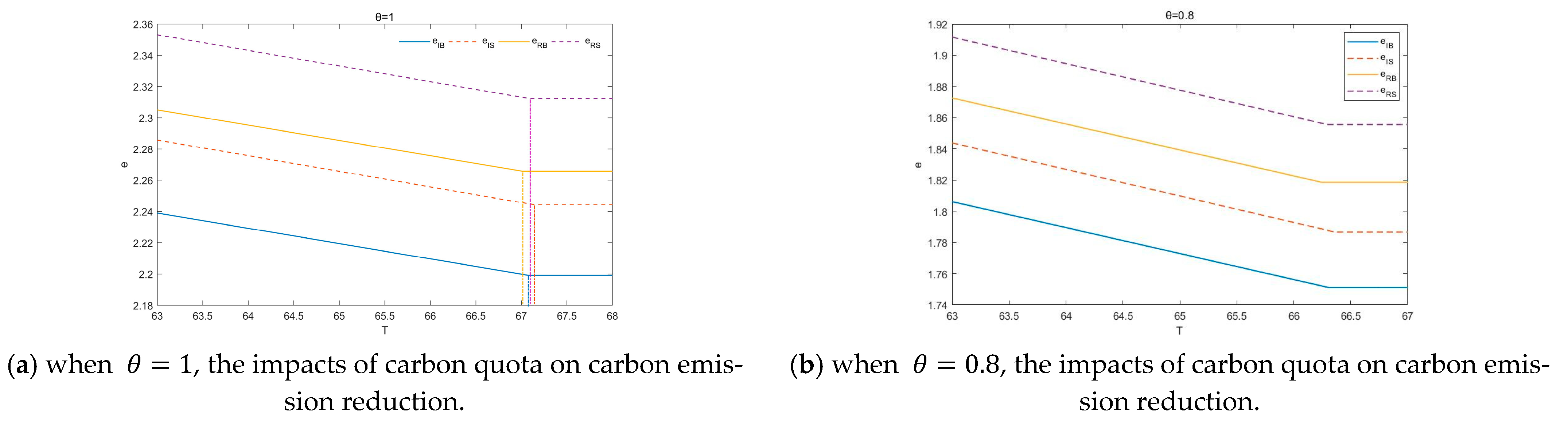
Let $\theta$ equal 0.3, 0.5, 0.8 and 1, respectively, according to the parameter settings. The effects of the carbon quota on the optimal service fee, emission reduction and business volume are shown in the figures. As can be seen from Figure 2, with the relaxation of the carbon quota policy, the carbon emission reduction decreases, indicating that when the carbon quota policy formulated by the government is relatively loose, 3PL can more easily meet the carbon emission standard, so 3PL will reduce its carbon emission reduction investment in order to obtain more profits. Among the effects, the carbon emission reduction when the government conducts overall supervision is significantly smaller than the carbon emission reduction when the government conducts separate supervision of 3PL. This is because, with overall supervision, the responsibility for emission reductions and the pressure regarding carbon emissions lie with 4PL. For 3PL, there is no risk of direct punishment for a decrease in emission reduction, so 3PL will neglect carbon emission reduction. When separate supervision is carried out, the pressure to reduce emissions is directly placed on 3PL. Therefore, compared with the overall supervision situation, 3PL will take more initiative in emission reduction during separate supervision.

As can be seen from Figure 3, with the relaxation of carbon quota policy, the optimal business volume of 3PL increases. Among the factors, the overall regulation or separate regulation by the government has little impact on the optimal business volume of 3PL. The optimal business volume under separate regulation by the government is slightly larger than that under overall regulation, while the choice of 3PL’s financing strategy has a greater impact on its business volume. As can be seen from the figure, the optimal business volume when 3PL chooses 4PL financing is greater than it is when bank loans are made.

As can be seen from Figure 4, with the relaxation of the carbon quota policy, the unit service fee charged by 4PL to 3PL increases, and the unit service fee in the overall supervision scenario is greater than that in the separate supervision scenario. This is because 4PL undertakes the risk of being punished for excess carbon emissions when the carbon quota policy is tightened during the scenario of overall supervision by the government. Therefore, 3PL is encouraged to carry out carbon emission reduction activities by reducing its service price. When the government separately regulates 3PL, it may reduce carbon emissions by reducing its business volume to avoid being punished. When 3PL reduces its business volume, 4PL’s profits will also decrease, so 4PL will reduce its service price. This represents a side incentive for 3PL to carry out carbon reduction activities. It can be seen that the more stringent the carbon quota policy is, the stronger is the awareness of the carbon emission reduction of enterprises. 3PL will increase its carbon emission reduction investment and reduce its business volume to reach the carbon quota standard; 4PL will encourage 3PL to reduce its carbon emissions using service fees.

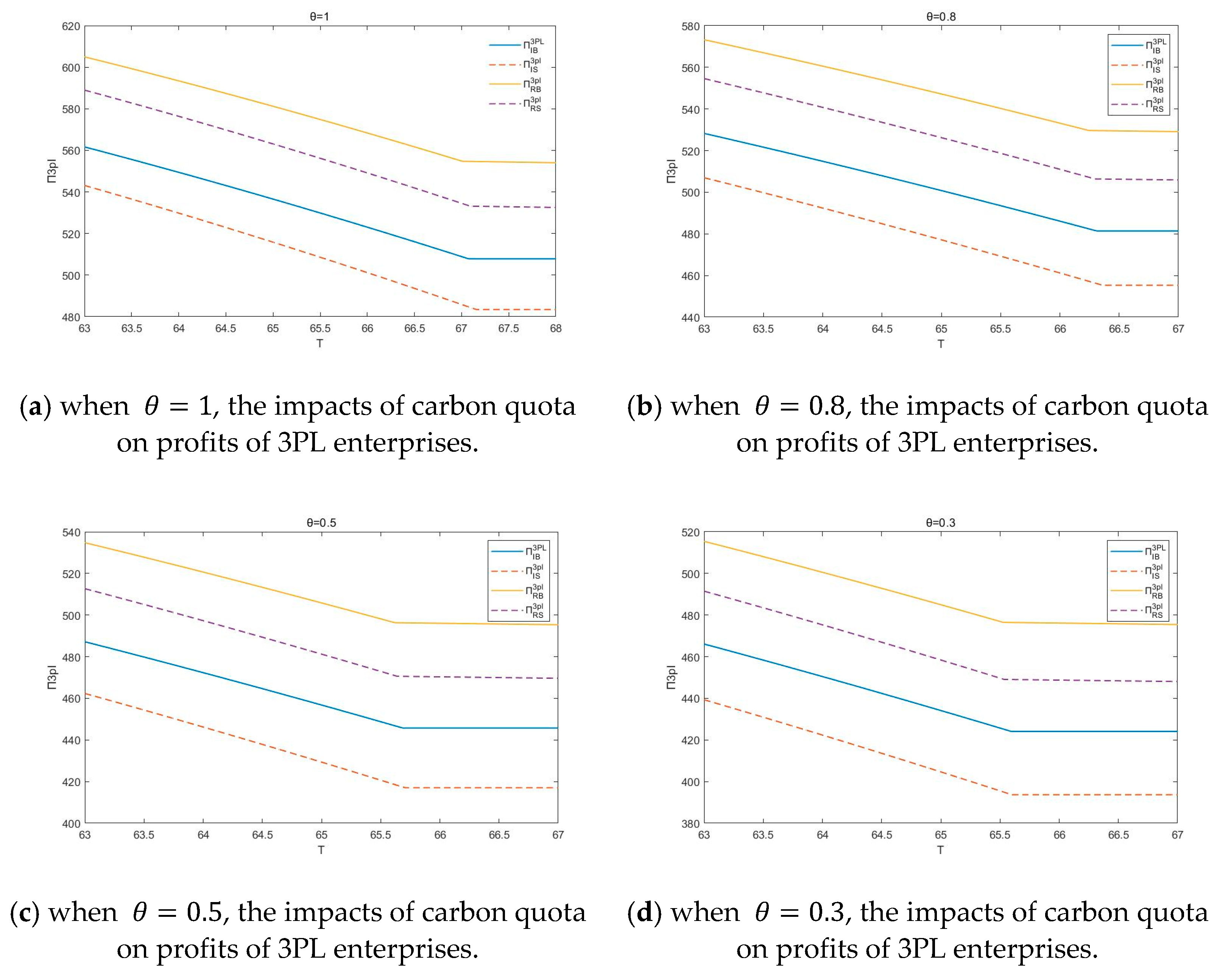
The impact of a carbon emission cap on 3PL’s and 4PL’s profits is shown in Figure 5 and Figure 6. As can be seen from Figure 5 and Figure 6, 3PL obtains higher profits when the government separately supervises 3PL, while 4PL obtains higher profits when the government chooses overall supervision. With the relaxation of the carbon quota policy, 3PL’s profits decrease, which is due to the increase in the cost incurred by 3PL due to the increase in the service price. Regardless of whether the government conducts overall supervision or separate supervision, for 3PL and 4PL, both enterprises can obtain higher profits when 3PL chooses 4PL financing.

(2) The influence of consumers’ green preference ($\theta$) on the optimal decision and profit of enterprises.

We set the following parameters: $c_l=10$, $a=160$, $k=6$, $p_c=0.7$, $r=0.05$, $T=55$, $e_0=3$. The influence of consumers’ green preference on 4PL’s unit service fee and 3PL’s carbon emission reduction and business volume are shown in Figure 4. As can be seen from Figure 7, the higher the consumers’ green preference level, the higher the carbon emission reduction of 3PL and the smaller its business volume. With the increasing green awareness of consumers, there are higher requirements for “green products”; when the “green” requirements of consumers cannot be met, the business volume of enterprises will decline, so 3PL will increase its investment in green emission reduction in order to obtain more consumers. 4PL also hopes to obtain more consumers, so it will encourage 3PL to increase its carbon emission reduction investment in the form of reduced service fees.

As can be seen from Figure 8, as the consumers’ green preference level increases, the profits of 3PL increase, while the profits of 4PL decrease. This indicates that with the increase in consumers’ green preference, 3PL’s business volume decreases, but it can obtain more profits through higher pricing. For 4PL, the decrease in business volume will lead to a decrease in corporate profits.

(3) The influence of consumers’ green preference ($e_0$) on the optimal decision and profit of enterprises.

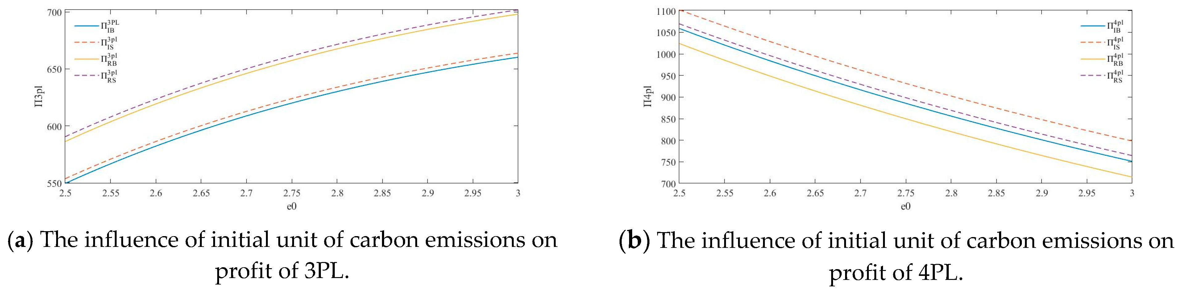
We set the following parameters: $c_l=10$, $a=100$, $k=6$, $p_c=0.7$, $r=0.05$, $\theta =1$, $T=55$. The impacts of the initial unit of carbon emissions on service price, carbon emission reduction and business volume are shown in Figure 9. It can be seen from Figure 6 that with the increase in the initial unit of carbon emissions, the carbon emission reduction of 3PL first increases and then decreases, and the optimal business volume decreases. This shows that when the initial unit of the carbon emissions of an enterprise is small, the enterprise can easily reach the carbon quota standard, and the enterprise can reduce carbon emissions by reducing business volume.

As can be seen from Figure 10, as the initial unit of carbon emissions of 3PL increases, the profit of 3PL increases, first rapidly and then slowly, and the profit of 4PL decreases accordingly. This is because when the initial unit of carbon emissions is small, the enterprise can easily reach the carbon quota limit, so the carbon emission reduction investment is less. Enterprises need to invest a lot of money in carbon emission reduction, and in order to meet the carbon quota standard, some business volumes will be reduced, resulting in a decline in corporate profits.

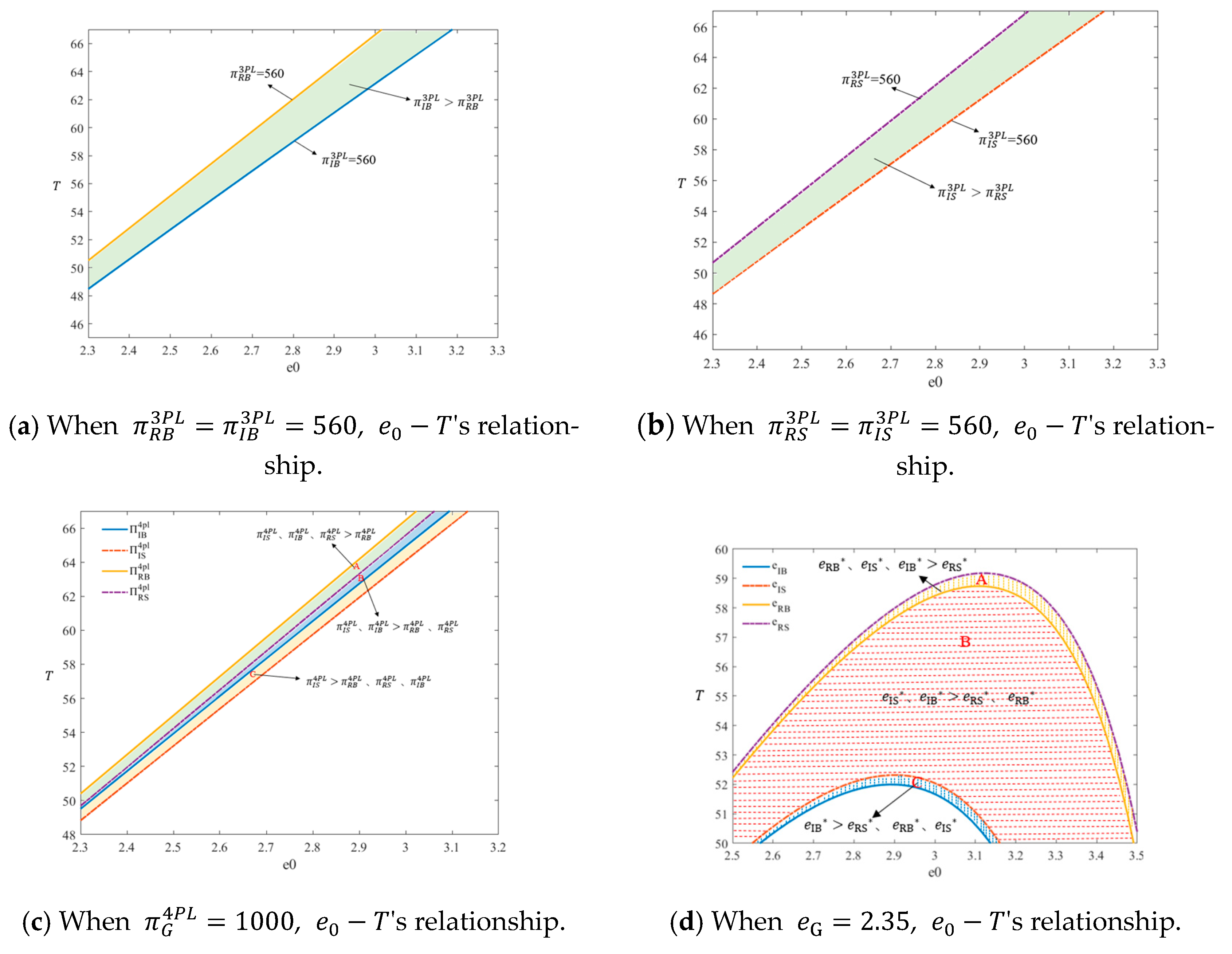
If ${\pi }_G^{3PL}=560$, ${\pi }_G^{4PL}=1000$, and $e_{\mathrm{G}}=2.35$, the relationship $e_0-T$ is shown in Figure 11. Figure 11a,b show the relationship between the two financing strategies of $e_0-T$ under different supervision modes when the profit value of 3PL is 560, that is, ${\pi }_G^{3PL}=560$. It can be seen from the figure that when the value of $e_0-T$ is in the shaded area, ${\pi }_{IB}^{3PL}{>\pi }_{RB}^{3PL}$, ${\pi }_{IS}^{3PL}{>\pi }_{RS}^{3PL}$. Figure 11c shows the relationship between the four sub-games of $e_0-T$ when the profit of 4PL is 1000, that is, ${\pi }_G^{4PL}=1000$. It can be seen from the figure that when the value of $e_0-T$ is in region A, ${\pi }_{IS}^{4PL}, {\pi }_{IB}^{4PL}, {\pi }_{RS}^{4PL}>{\pi }_{RB}^{4PL}$. When $e_0-T$ is in region B, ${\pi }_{IS}^{4PL}, {\pi }_{IB}^{4PL}>{\pi }_{RB}^{4PL}, {\pi }_{RS}^{4PL}$. When the value of $e_0-T$ is in the C region, ${\pi }_{IS}^{4PL}>{\pi }_{RB}^{4PL}$, ${\pi }_{RS}^{4PL}$, ${\pi }_{IB}^{4PL}$. Figure 11d shows the relationship $e_0-T$ when the carbon emission reduction values of the four sub-games are all 2.35; that is, when $e_{\mathrm{G}}=2.35$, it can be seen from the figure that when $e_0-T$ values are in region A, ${e_{\mathrm{R}\mathrm{B}}}^{\mathrm{*}}, {e_{\mathrm{I}\mathrm{S}}}^{\mathrm{*}}, {e_{\mathrm{I}\mathrm{B}}}^{\mathrm{*}}>$ ${e_{\mathrm{R}\mathrm{S}}}^{\mathrm{*}}$. When $e_0-T$ is in the B region, ${e_{\mathrm{I}\mathrm{S}}}^{\mathrm{*}}, {e_{\mathrm{I}\mathrm{B}}}^{\mathrm{*}}>$ ${e_{\mathrm{R}\mathrm{S}}}^{\mathrm{*}}$, ${e_{\mathrm{R}\mathrm{B}}}^{\mathrm{*}}$. When $e_0-T$ is in the C region, ${e_{\mathrm{I}\mathrm{B}}}^{\mathrm{*}}>$ ${e_{\mathrm{R}\mathrm{S}}}^{\mathrm{*}}$, ${e_{\mathrm{R}\mathrm{B}}}^{\mathrm{*}}, { e_{\mathrm{I}\mathrm{S}}}^{\mathrm{*}}$.

6. Discussion

This paper mainly explores the problem of capital constraint in the process of the sustainable development of enterprises. In the process of sustainable development, small and medium-sized logistics enterprises face serious financing constraints. However, there is little research on this in the literature of green finance. This paper takes small and medium-sized logistics enterprises that need to transform their processes to sustainable development processes as the research object, and considers the scenario wherein 4PL provide financing. This paper constructs a Stackelberg game to study the green financing strategy of small and medium-sized logistics enterprises. In the model, small and medium-sized logistics enterprises have two strategies: bank financing or 4PL financing. The government has two strategies: overall supervision or separate supervision. By solving the above model, this paper finds the following:

(1) Under the two supervision methods, the separate supervision method is more conducive to carbon emission reduction, and the optimal decision of enterprises is related to the amount of the carbon quota. When the carbon emission policy set by the government is loose, the optimal decisions of 3PL enterprises are not affected by the carbon quota, so enterprises can make decisions on the basis of maximizing their profits. When the government’s carbon emission policy is strict, 3PL enterprises must maximize their profits according to the carbon emission cap.

(2) Under the two financing strategies, 3PL enterprises’ choice of 4PL financing is more conducive to carbon emission reductions. When 3PL enterprises choose 4PL financing, compared with bank financing, 4PL enterprises will offer lower service prices, which reduces the cost incurred by 3PL enterprises.

(3) When the government chooses “separate supervise”, 3PL enterprises can obtain lower unit service fees, reduce their costs and expenditures and obtain higher profits; at the same time, this scenario is more conducive to carbon emission reductions. When the government chooses “overall supervise”, because 4PL enterprises bear the risk of being penalized for exceeding carbon emissions, the carbon quota policy cannot effectively encourage 3PL enterprises to carry out emission reduction activities, resulting in a lower carbon emission reduction effect than that produced by the direct supervision of 3PL enterprises. From a comprehensive point of view, the strategy combination of “separate supervise” and “4PL financing” is the most conducive to carbon emission reduction.

The contribution of this paper is its consideration of the influence of different governmental supervision methods on the financing decisions of enterprises. Government policies have a guiding effect on the sustainable development of enterprises. Therefore, this paper puts forward two different supervision methods, hoping to provide some references for the governmental supervision model. At the same time, 4PL financing is considered in this paper. These contributions not only provide a reference for breaking the financial constraints present in the sustainable transformation of logistics enterprises but also for the diversification of the development of financing methods of the green supply chain in the future. However, this paper still has some limitations. The Stackelberg game model only considers a supply chain system composed of a single 4PL enterprise and a single 3PL enterprise, and the market demand is assumed to be certain. It also assumes that the interest rate of 4PL financing is the same as that of bank financing.

7. Conclusions

This paper explores the financing strategy selection of logistics enterprises facing green capital constraints in the process of sustainable development, analyzes the optimal decision of enterprises, and finds that the government’s carbon quota policy and supervision mode will affect the optimal decisions of enterprises. This paper can provide some suggestions for reference: First of all, for the allocation of carbon allowances, it is necessary to consider the current carbon emission levels of enterprises to formulate appropriate carbon quota policies, so as to play a restrictive role in the carbon emissions of enterprises. Secondly, from the perspective of the choice of regulatory methods, it is intuitive to see that the overall regulatory approach has fewer regulatory objects and is more convenient for management, but the carbon emission reduction effect under overall supervision is smaller than that under separate supervision. Because 4PL enterprises bear the risk of being punished in the overall supervision scenario, in order to balance the risk, 4PL enterprises will charge more service fees. This is harmful to the ability of 3PL enterprises to undertake the project of carbon emission reduction. Therefore, the government and 4PL enterprises should take some measures to encourage 3PL enterprises to carry out carbon emission reduction activities. For example, the government and 4PL enterprises can incentivize 3PL enterprises according to the amount of 3PL emission reduction and reduce service fees, so as to strengthen the cooperation between upstream and downstream enterprises and promote the sustainable development of the supply chain.

This paper only considers the situation in which logistics parks need to rely on 3PL emission reductions to reduce their carbon emissions. However, due to the different management methods of logistics parks, some logistics parks can also independently reduce their emissions in some transport links. Therefore, more diverse types of logistics parks and 3PL emission reduction forms can be considered in the future, and different financing strategies can be explored to promote the overall sustainable development of the supply chain. In addition, only 4PL financing, a green supply chain financing method, is considered in this paper, and more diversified financing services can be further studied and innovated in future studies. At the same time, 4PL, as an integrator of supply chain services, has great advantages in resource integration. Therefore, in the future, we can conduct more in-depth research on the impact of 4PL’s financial services on the sustainable development of the supply chain.

References

1. Available online: https://www.greenpeace.org.cn/wp-content/uploads/2023/06/express-industry-emissions.pdf (accessed on 1 February 2024).
2. Xue, C.H.; Wei, P. Research on green credit strategy of Chinese commercial banks based on game model. Financ. Theory Pract. 2020, 5, 75–81. [Google Scholar]
3. Xu, R.Z.; Wang, S.; He, T.T. Research on dynamic mechanism of sustainable development of small and medium-sized enterprises from the perspective of green supply chain finance. Financ. Theory Pract. 2022, 1, 76–86. [Google Scholar]
4. Chen, S.; Du, J.; He, W.; Siponen, M. Supply chain finance platform evaluation based on acceptability analysis. Int. J. Prod. Econ. 2022, 243, 108350. [Google Scholar] [CrossRef]
5. Dong, J.; Zhang, Q. Sustainable Development of the Real Economy: Supply Chain Finance and Enterprise Financialization. Sustainability 2024, 16, 3574. [Google Scholar] [CrossRef]
6. Song, H. The Development Trend of Supply Chain Finance in China. China Bus. Mark. 2019, 33, 3–9. [Google Scholar]
7. Li, J.; Wang, Y.; Feng, G.; Wang, S.; Song, Y. Supply chain finance review: Current situation and future trend. Syst. Eng. Theory Pract. 2020, 40, 1977–1995. [Google Scholar]
8. Fang, L.; Xu, S. Financing equilibrium in a green supply chain with capital constraint. Comput. Ind. Eng. 2020, 143, 106390. [Google Scholar] [CrossRef]
9. Cheng, J.; Hong, W.; Cheng, J. Optimal Green Input Level for a Capital-Constrained Supply Chain Considering Disruption Risk. Sustainability 2023, 15, 12095. [Google Scholar] [CrossRef]
10. Lai, Z.X.; Lou, G.X.; Ma, H.C.; Chung, S.H.; Wen, X.; Fan, T. Optimal green supply chain financing strategy: Internal collaborative financing and external investments. Int. J. Prod. Econ. 2022, 253, 108598. [Google Scholar] [CrossRef]
11. Zhang, M.; Li, J.; Liu, F.; Nan, J.; Jiang, J. Pricing and Financing Strategies of Dual-Channel Green Supply Chain with Risk Aversion and Consumer Preferences. Sustainability 2024, 16, 5602. [Google Scholar] [CrossRef]
12. An, S.M.; Li, B.; Song, D.P.; Chen, X. Green credit financing versus trade credit financing in a supply chain with carbon emission limits. Eur. J. Oper. Res. 2020, 292, 125–142. [Google Scholar] [CrossRef]
13. Zhou, T.; Tao, M.; Meng, X.Q. Research on low-carbon financing strategies of manufacturers considering capital constraints under carbon trading regulations. Financ. Theory Pract. 2022, 9, 44–56. [Google Scholar]
14. Zhang, Y.L.; Hu, X.Q. Research on supply chain decision-making considering manufacturers’ financial constraints under carbon quota policy. J. Hefei Univ. Tech. (Nat. Sci. Edit.) 2022, 45, 1413–1421. [Google Scholar]
15. Lin, Q.; Zhao, Z.Z.; Huo, B.F.; Lin, X.G.; Li, W.Z. Cooperative emission reduction strategies of retailers considering carbon trading policies: Financing emission reduction or technology emission reduction. Syst. Eng. Theory Pract. 2024, 44, 986–1005. [Google Scholar]
16. Qin, C.; Hong, Y.-T. Quadripartite Evolutionary Game of Sustainable Development of Supply Chain Finance with Government Participation. Sustainability 2023, 15, 3788. [Google Scholar] [CrossRef]
17. Kang, H.; Jung, S.Y.; Lee, H. The Impact of Green Credit Policy on Manufacturers’ Efforts to Reduce Suppliers’ Pollution. J. Clean. Prod. 2019, 248, 119271. [Google Scholar] [CrossRef]
18. Ma, W.M.; Zhang, R.R.; Cheng, Z.R. Analysis of Internal and External Funding Mechanisms Considering Green Consumer Loyalty: A Game-Theoretic Approach. IEEE Access 2019, 8, 2931–2947. [Google Scholar] [CrossRef]
19. Meng, Q.F.; Li, M.W.; Liu, W.Y.; Li, Z.; Zhang, J. Pricing policies of dual-channel green supply chain: Considering government subsidies and consumers’ dual preferences. Sustain. Prod. Consum. 2021, 26, 1021–1030. [Google Scholar] [CrossRef]
20. Huang, S.; Fan, Z.P.; Wang, N.N. Green subsidy modes and pricing strategy in a capital-constrained supply chain. Transport Res. E-Log. 2020, 136, 101885. [Google Scholar] [CrossRef]
21. Wang, H.; Gan, W.; Wang, X.; Liu, D. A low carbon supply chain subsidy strategy for SMEs that considers both manufacturers and retailers under carbon cap-and-trade. Sci. Tech. Manag. Res. 2023, 43, 193–202. [Google Scholar]
22. Long, J.R.; Zhong, C.B.; Bilal, A.; Irfan, M.; Nazir, R. How do green financing and green logistics affect the circular economy in the pandemic situation: Key mediating role of sustainable production. Eco. Res. Ekon. Istraz. 2022, 35, 3836–3856. [Google Scholar]
23. Zhu, X.W.; Du, J.G.; Ali, K.; Kirikkaleli, D. Do green logistics and green finance matter for achieving the carbon neutrality goal? Environ. Sci. Pollut. Res. 2023, 30, 115571–115584. [Google Scholar] [CrossRef] [PubMed]
24. Yang, H.X.; Duan, W.Y. Research on financing strategies of green supply chain for manufacturers’ capital constraints. Oper. Res. Manag. 2019, 28, 126–133. [Google Scholar]
Figure 1. Game event sequence diagram.
Sustainability 16 06432 g001
Figure 2. Impacts of carbon quota on carbon emission reduction.
Sustainability 16 06432 g002aSustainability 16 06432 g002b
Figure 3. Impacts of carbon quota on business volume.
Sustainability 16 06432 g003
Figure 4. Impacts of carbon quota on service price.
Sustainability 16 06432 g004
Figure 5. Impacts of carbon quota on profits of 3PL enterprises.
Sustainability 16 06432 g005
Figure 6. Impacts of carbon quota on profits of 4PL enterprises.
Sustainability 16 06432 g006
Figure 7. Influence of consumers’ green preference on carbon emission reduction, business volume and service price.
Sustainability 16 06432 g007
Figure 8. Influence of consumers’ green preference on profits of 3PL and 4PL enterprises.
Sustainability 16 06432 g008
Figure 9. Influence of initial unit of carbon emissions on carbon reduction, business volume and service price.
Sustainability 16 06432 g009
Figure 10. Influence of initial unit of carbon emissions on profits of 3PL and 4PL enterprises.
Sustainability 16 06432 g010
Figure 11. e 0 T ’s relationship.
Sustainability 16 06432 g011