1. Introduction
Interchange mainline accidents are more frequent than ramp accidents [
1], and about 40% of mainline traffic accidents are caused by various types of mandatory lane changes (MLCs). Due to the driver’s concern about missing an exit, continuous lane changes and emergency lane changes often occur in front of the interchange diversion area. Continuous lane changing usually involves interruptions in the lane changing process [
2], and emergency lane changing, such as the driver starting to change lanes only after approaching the exit, usually involves a drastic change in speed [
3].These are defined as invalid lane changes, which typically expose vehicles to prolonged vehicle interactions and generate traffic oscillations, leading to an increased risk of collision [
4]. For heavy-duty trucks, they not only have a high accident rate and mortality rate on interchange sections but also easily lead to regional traffic paralysis and may cause secondary traffic accidents and major safety accidents. This means that highway interchanges pose a serious threat to the safety of heavy trucks while changing lanes and have become a pain point that restricts the improvement of highway safety and the healthy development of freight logistics.
The collision risk of MLCs is essentially caused by the instability of vehicle driving caused by the geometric design [
5], and the main characteristic of geometric design factors is their long-term stability. Scholars have studied geometric factors related to MLCs through simulation driving or simulation techniques, such as curve radius and curve bending direction [
6], as they affect the psychological workload of drivers when changing lanes to the right. In addition, the geometric design differences of the main upstream and downstream road sections can also affect the driving difficulty for drivers [
7]. According to the investigation, if sudden changes in road characteristics violate the driver’s expectations, road accidents tend to be more frequent, which can be described by the consistency index of geometric design [
8]. The evaluation method for design consistency can be measured by the difference between continuous operating speed and design speed [
7,
8], and the degree of coordination with the overall alignment of the highway section can also be quantified by the curve length and slope change rate. Inconsistent designs lead to frequent and rapid deceleration of vehicles, and similar influencing factors include daily traffic flow [
9]. However, the existing lane changing analysis is based on simplified rigid body models and assumed trajectories, ignoring the heterogeneity of heavy-duty trucks in terms of vehicle dynamics and driving trajectories. For heavy-duty trucks, the safety of MLCs in interchange areas is not yet clear about which interchange design elements affect the degree of safety and how they affect it, resulting in difficulty in accurately controlling the safety margin of design indicators. In recent years, the density of highway networks has gradually increased, and the complexity of the geometric design between interchanges has also increased. The geometric design of interchange areas not only includes horizontal and vertical lines but also involves functional sections such as transition sections, acceleration and deceleration lanes, and weaving areas. The adjustment of one design element often affects the entire interchange design. Therefore, it is necessary to focus on analyzing the impact of geometric design on the exposure time and validity of heavy-duty truck MLCs and analyzing other design elements from a global safety perspective to further improve the traffic safety of interchange areas.
The existing research is mostly based on simulated driving or simulation techniques or on investigating the influencing factors of lane changing over a certain length of area. The emergence of full time-domain trajectory big data in the digital era provides unprecedented opportunities to solve this problem. Among numerous driving characteristic data collection technologies, the high-precision coordinate positioning data obtained through heavy-duty freight floating vehicles in the full time domain and all road sections has a series of significant advantages. Compared with general data, these data have multiple characteristics, such as full time-domain, large range, and high accuracy, which are conducive to comprehensively and accurately grasping the lane changing characteristics of heavy-duty trucks in day and night environments, various interchanges, and different road sections. In addition, analyzing the MLC behavior of heavy trucks can represent the most adverse effects of behavior during the lane changing process in the interchange diversion area, which will guide the refined design of various elements of interchanges in the existing design guidelines. The survival analysis methods applied in the medical field have also achieved similar goals, such as using the Cox survival analysis to study the influencing factors of survival time after discharge in advanced cancer patients [
10]. The Cox proportional risk model is a commonly used survival analysis model used to study time-to-event data. Then, scholars in the field of transportation applied the traditional Cox model to conduct a similar analysis of lane change (LC) duration, used to model the relationship between the duration of LC occurrences and related features. But in the Cox model, it is assumed that the impact of covariates on survival time is linear and does not change over time. However, when there is a nonlinear relationship between covariates and survival time, it can lead to autocorrelation patterns in the residual of the model, affecting the estimation of model parameters and the reliability of confidence intervals [
10]. Fortunately, the baseline risk function in the Cox model allows for modeling the survival time of events as a combination function of time and covariates. In addition, a generalized additive model (GAM) can be represented by replacing the linear effects of the predicted variables with the sum of smooth functions. Therefore, combining a GAM with Cox proportional risk models can effectively handle the nonlinear relationship between the geometric design and lane changing survival time. The survey object of this study is the duration of ineffective MLCs before the interchange diversion area. We combine the standard model with the GAM [
11]. The GAM can use parameter smoothers to model geometric design covariates as nonlinear functions of mandatory lane change duration (MLCD). At the same time, time components are added to the model to consider the differences in covariates between day and night [
12].
The purpose of this article is to analyze the geometric design impact of MLCD of heavy trucks in the interchange diversion area based on the full time-domain trajectory big data of the interchange area, providing theoretical and methodological references for the fine design of interchanges. The main contributions of this study include the following:
(1) By introducing full time-domain, large-scale, and high-precision trajectory big data, this study explores the differences in MLC characteristics of heavy-duty trucks under different geometric elements of interchanges and day and night conditions. In addition, considering the influence of different combinations of geometric elements on different road sections, the impact mechanism of the geometric elements of interchanges on the exposure time of heavy truck MLCs was elucidated, providing an important theoretical basis for truly reflecting the lateral, dangerous behavior of heavy trucks on various road sections of interchanges.
(2) A duration model for MLCs in interchange areas has been established. On the basis of the standard Cox model, combined with the GAM, time-dependent function, and shared fragility parameters, the nonlinear impact of geometric design on MLCs, time-varying effects, and heterogeneity of driver lane changing are considered separately. This provides a more practical and feasible analysis method for analyzing the safety of interchanges and uses actual operating trajectory modes instead of traditional ideal trajectory radii.
The rest of this article is organized as follows.
Section 2 provides a review of the literature,
Section 3 proposes our improvement methods,
Section 4 introduces data preparation and experimental results,
Section 5 discusses the results, and
Section 6 presents our conclusions and suggestions for future work.
3. Methods
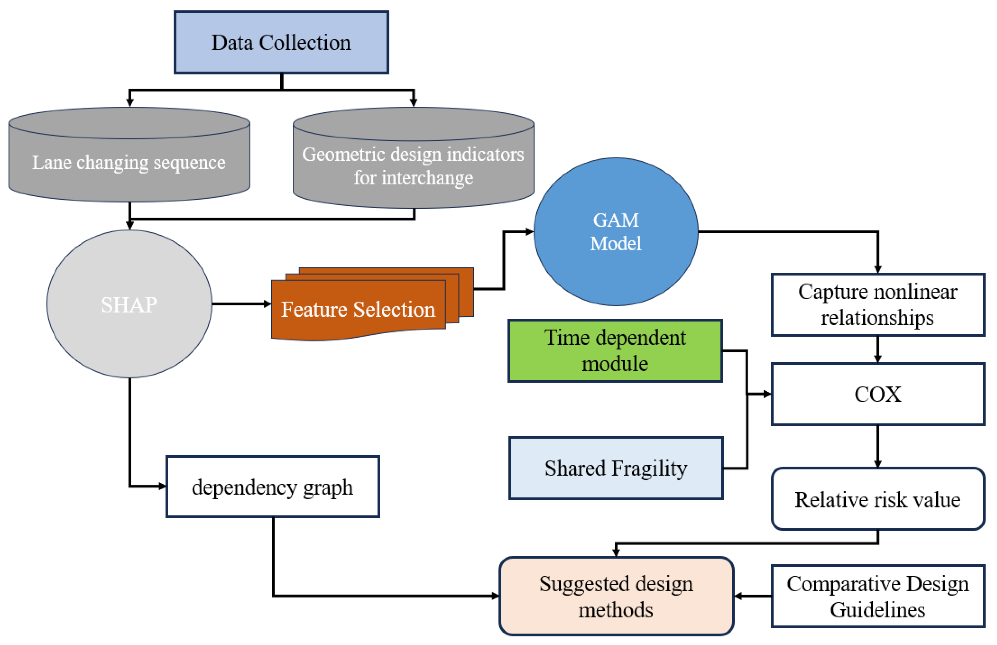
Our method steps are shown in
Figure 1. First, heavy truck trajectory data were collected from 38 interchange areas, which included more than 50 attributes per driver. Then, the data were cleaned and matched with the map to obtain MLC sequences, and the feature selection was carried out through the SHapley Additive exPlanations (SHAP) algorithm. The final data set included 18 variables for each record. Then, the GAM was used to nonlinearize the characteristics, and the time-dependent module was introduced to consider the circadian conditions, as well as the shared fragility to modify the model to obtain the relative risk value of geometric characteristics. Finally, compared with the guidelines of interchange, suggestions for design improvement were put forward.
3.1. Feature Selection
The SHAP model is commonly used to explain the importance of complex model features, such as deep-learning models [
10]. Due to its powerful parsing and visualization capabilities, some scholars have gradually applied it to traffic safety research in recent years. The calculation of SHAP values is based on iterating the combinations of all possible feature subsets, thus comprehensively considering the impact of each feature under different combinations.
In this study, we used the Scikit Learn Wrapper interface provided by XGBoost (version 1.4.0) to train a random forest model and selected features based on two target variables (MLCD and MLC validity). Then, the SHAP library in Python (version 3.9.5) generated SHAP values for each sample. The SHAP value represents the degree to which each feature affects the model output. The SHAP value is displayed in the decision graph, which provides a detailed view of the internal workings of the model and demonstrates a large number of feature effects that are clearly visualized through multi output prediction [
31]. This process used 30 features, ranked in descending order of their impact on the model. A total of 18 features were rated as having the greatest impact by both algorithms and were therefore selected for survival analysis. Finally, we used Pearson correlation coefficient to test the correlation between these variables and discarded three highly correlated variables, as shown in
Table 1. Therefore, this method identifies the variables for survival analysis modeling.
3.2. Generalized Additive Models (GAMs)
With the emergence of nonlinear effects in covariates, linear regression models cannot give promising results, so it is necessary to introduce nonlinear descriptions, such as GAM, which enables us to fit the model with nonlinear smoothers without specifying specific shapes in advance. GAM solves this difficulty by allowing smoothing functions or smoothers in the linear prediction components of the regression model, as well as “unsmoothed” covariates. Therefore, the general equation of GAM can be written as:
where
is the predictor,
is the smoothing term associated with these predictors,
is the intercept,
is the residual error term,
is the dependent variable,
is the expected value, and
is the link function.
The smoothing term selects a parameter smoother, such as a multinomial, a fraction multinomial, a piecewise multinomial, or a B-sample. The penalty smoother is used to find the best value for the smoothing parameter, which controls the amount of smoothing, that is, how well the smoothing term fits the original predictor. The geometric design variables of the overpass area are fitted to the nonlinear function of the research target using the GAM method.
3.3. Survival Analysis
Survival analysis is widely used in the medical field to determine the factors influencing the survival time of cancer patients [
30]. In recent years, its analysis method has been used to analyze the survival period of lane changing. It can be used to estimate the end time of lane changing and the most relevant factors to risk in lane changing when the vehicle begins to shift lanes.
According to the concept of survival analysis, the elements of MLCD for truck survival analysis are defined as follows:
(1) Event and event duration: The starting point of the event is the moment when the vehicle begins to deviate from the lane. The endpoint is the moment when the lane changes to the target lane and returns to the positive direction. The time difference between the starting and ending points of an event is the duration of the event.
(2) Event result: Event result indicates whether the MLCs of vehicles on the exit ramp are effective. When the vehicle is unable to complete a lane change in the designated area, ; otherwise, .
3.3.1. Risk Models in Survival Analysis
The survival function
defines the survival outcome, where
is the time when the event occurred or was reviewed and
represents whether the event occurred (yes/no). Therefore, the survival function indicates how much time will pass before event
occurs. The formal survival function is given by the following equation:
The equation is the probability that the survival time
exceeds the time
. The danger function
represents the probability that the driver who is making a LC at time
will end the lane change before “time
”. The danger function is given by:
A similar question of interest is the relative risk (hazard ratio (
)) between LCs obtained by calculating proportional risk.
Provided the hazards of LC exposed to risk factor () compared to LC not exposed to risk factor () are not equal.
3.3.2. Time-Varying Cox Proportional Risk Model (T-Cox-PH)
Cox-PH regression determined the relationship between the risk function and the predictor, but Cox believes that the relationship between the risk function and the predictor is linear, which means that variables have a constant impact over time. Since violating this assumption may compromise the effectiveness of the model, we modeled the time-varying effects through interactions with time to compensate for the shortcomings of the standard Cox model.
We used the Time-Varying Cox Proportional Risk model to estimate the geometric impact of covariates on the validness of LC after lane departure. LC that is invalid during this period is considered the subject of review. We estimated the danger function
, which measures the probability of driver
ending a lane change after the time
measured from MLC
, as follows:
Among them, is the time when the exit ramp lane deviates, is the unique baseline risk for all drivers in the LC library, and is a function of the GAM that converts covariates into nonlinear relationships. is used to introduce some variables into time effects. It is assumed that the influence of is constant, while the influence of allows for variation with a certain function of the analysis time. If the model is a discrete duration model, such as a time-dependent Logit or Probit model, non-proportional hazards can be constructed through similar interactions with time.
3.3.3. Shared Frailty of Cox-PH
The frailty model is an extension of the Cox-PH model, in which potential heterogeneity is included as the random multiplication effect known as fragility. In our study, frailty corresponds to repeated LCs by the same driver. These LCs are grouped, and the observed results may be correlated within a group. This correlation is believed to be caused by potential covariates or omitted covariates (“frailty”) that are common when the same driver is admitted to the hospital. These potential covariates trigger an unobserved heterogeneity.
We focus on multivariate shared frailty model. The multivariate frailty model extends the Cox-PH model by multiplying it by the baseline hazard function
, so that the risk of LC also depends on the potential random variable, namely the frailty random variable
. Different frailty distributions represent different ways of expressing unobserved heterogeneity and affect observed covariates in different ways. Therefore, the weak distribution will reduce or increase the risk for each driver, depending on
< 1 or
> 1. The weak danger function
of driver
’s
th LC is represented as:
Over time, the fragility value remains constant and is shared among each driver’s LCs. Therefore, assuming the sub-condition, it is assumed that the survival duration of the driver
’s LC is independent [
32]. For driver
of LC
, the conversion between the hazard function
and survival function
at the driver’s level is given by the following equation:
The survival function
S of the total driver is given by the following equation:
We tested two distributions of the frailty random variable
—with a mean of 1 and a variance of θ unknown gamma and Gaussian distributions. We reported the results of the Gaussian distribution and indicated that these results are very similar to those obtained using the gamma distribution. We used the penalty partial likelihood method running on the R “survival” and lifeline packages in Python to estimate the shared frailty model [
29].
4. Experiment Results
4.1. Data Preparation
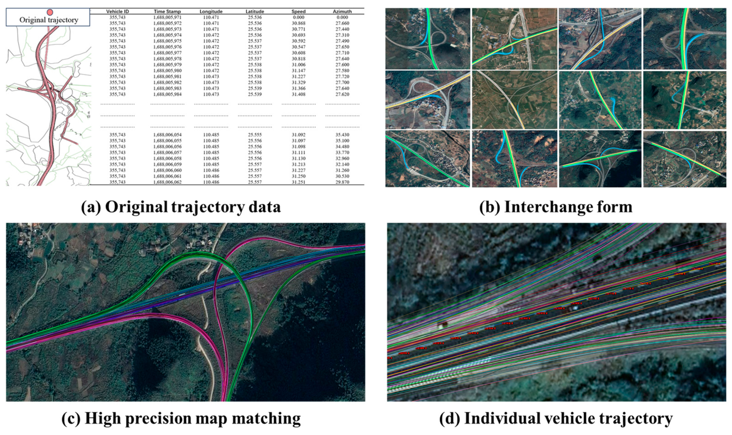
The data in this article are the floating vehicle trajectory data of heavy vehicles, collected from 1 June 2023 to 1 September 2023, with a sampling frequency of 1 Hz, positioning accuracy <1 m, and speed measurement accuracy of 0.2 m/s. The trajectory covers over 140 km of highways and is obtained by the onboard GPS of heavy trucks. As shown in
Figure 2a, our data include basic information such as longitude and latitude, vehicle ID, vehicle speed, heading angle, etc. The positions of these trajectories can match the road geometry design data, weather, accidents, and traffic volume information provided by the road section management company. Compared to the HighD [
21] and NGSIM [
33] datasets, the floating vehicle trajectory data cover a longer road segment, have a complete time range, and come with rich spatial information. This provides the possibility to study the impact of different spatial position attributes on the trajectory, which is the advantage of our data. As shown in
Figure 2b, our data include complex forms of interchanges, covering 38 interchanges (68 exit ramps) (only a few are listed). In addition, we use the “Pyautocad” library in Python to display all trajectories on CAD maps and then import them into Ovi Maps. As shown in
Figure 2d, each interchange was passed by an average of 10,000 different heavy trucks within a month, and we used data from a total of 3 months. Finally, we use map matching technology to divide the trajectory into different paths as shown in
Figure 2c.
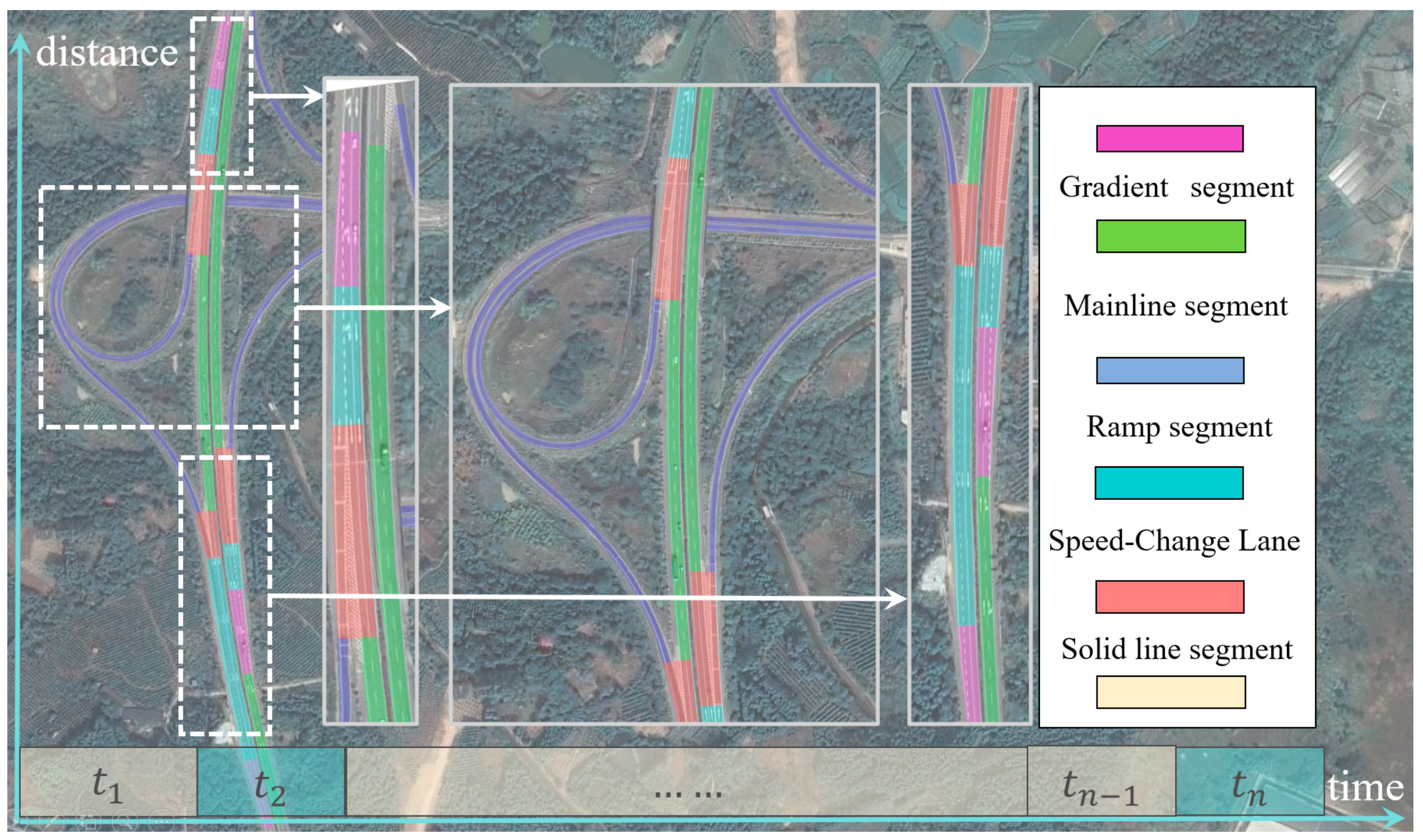
As shown in
Figure 3, the geometric elements in front of each interchange diversion area include the mainline section, gradient section, deceleration lane section, and solid line section (where lane changing is prohibited). In addition, based on the data of the road centerline, a road center stake system is established every 10 m. The purpose of establishing a pile system is to determine the lane changes of vehicles and their lateral positions relative to the road centerline and convert these points into a Frenet coordinate system with the road centerline as the reference line. To minimize lane change (LC) recognition errors, we have established multiple rules for LC detection, as shown below:
Step 1: Calculate the lateral offset of the continuous trajectory from the road centerline per second. Defines that the outward offset is negative, and the inward offset is positive.
Step 2: Sum the lateral continuous offsets and extract the travel data of these trajectories when the cumulative lateral deviation exceeds the width of the vehicle.
Step 3: For travel processes in Step 2 where the cumulative lateral offset reaches the vehicle’s width, determine the lane number at the starting point and the lane number at the ending point. If these two lane numbers are different, classify it as a lane change (LC).
Step 4: For the collected LC data, the right lane change of vehicles approaching the exit ramp before passing through the exit ramp sign and before the diversion nose is defined as a mandatory lane change.
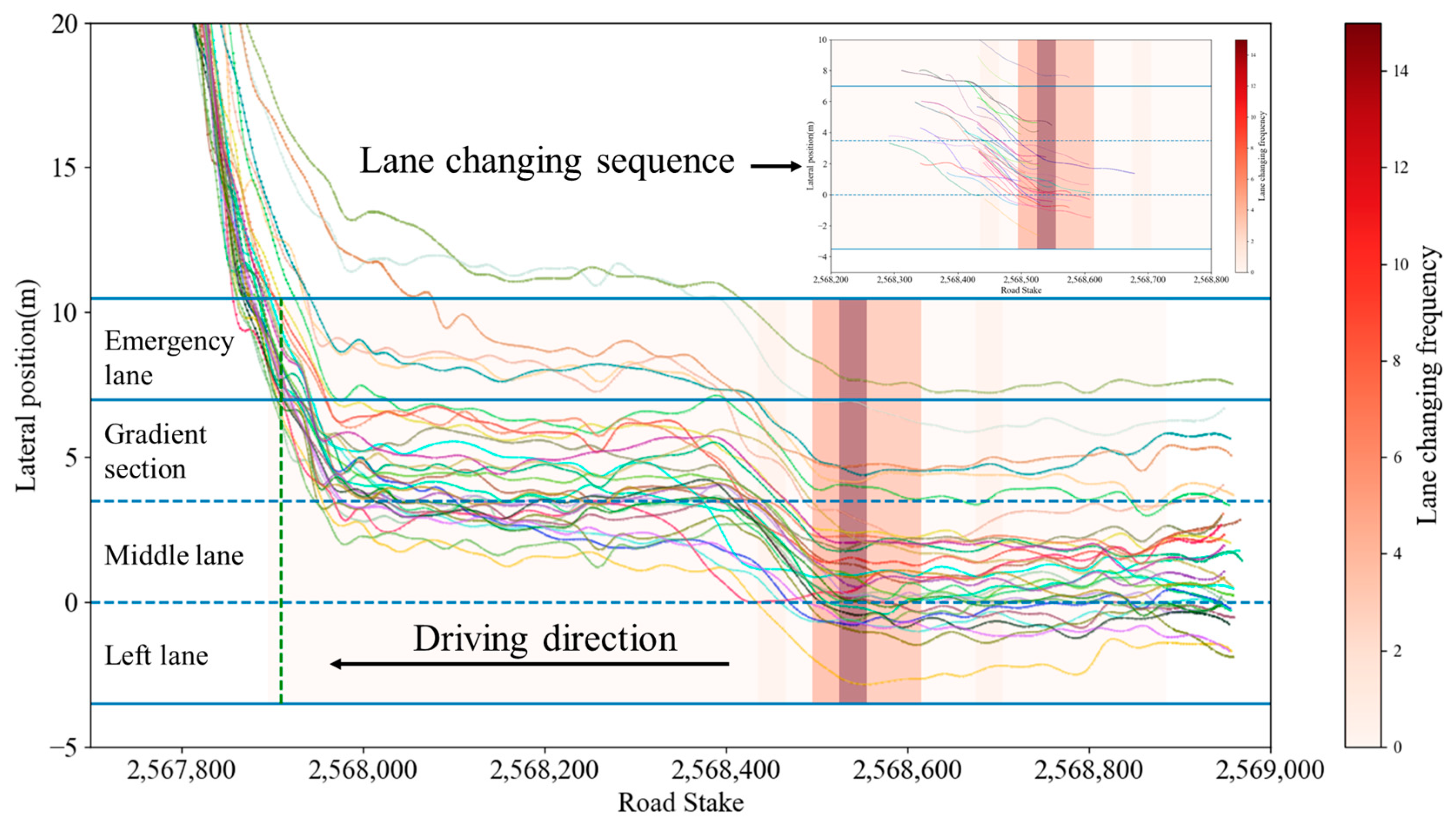
As shown in
Figure 4, we present an example of extracting the forced lane change behavior in front of the interchange diversion area. This figure contains the complete trajectory of the floating truck in the diversion area and the lane change offset sequence extracted through rules. Each region displays the frequency of the starting position of lane change through a heatmap. Through this method, the lane changing trajectories of all interchanges can be extracted.
4.2. Descriptive Statistics
This study extracted a total of 5845 cases of mandatory and FLC of heavy-duty trucks in different interchange diversion areas. Considering the differences in left and right lane changing types [
34], this study focuses on comparing the duration of free right lane changing and mandatory lane changing.
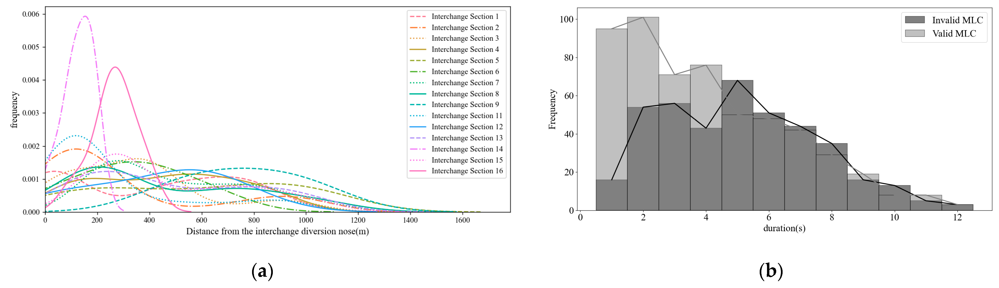
Figure 5 shows that the duration of MLCs for heavy-duty trucks is 0.5~1 s shorter than FLC, and the coefficient of variation for MLCD is higher. From the location of LC,
Figure 6a shows that the MLC in front of the interchange diversion area is mainly distributed around 170 m~800 m.
Figure 6b shows that the invalid lane change duration is concentrated at 5 s, which is about 3 s longer than the valid MLCD. In addition, compared to the MLCD of small cars that have been studied [
24], the MLCD of the heavy-duty trucks is about 0.6 s longer than small cars.
4.3. Feature Selection
Figure 7a,c show the SHAP summary of the duration and validity of MLCs, respectively. The results in the figures indicate the importance of the variables.
Figure 7b,d represent decision graphs. In the “decision_plot” function of the SHAP library, the link parameter is used to specify the link function to be displayed. The LC duration uses the “identity” link function, and the MLC validity uses the “logit” binary classification function. Specifically, each horizontal line in the decision graph represents the influence of a feature. The position of the line represents the impact of a given feature value on the model output. If the line is biased to the left, it indicates that the feature value has a negative impact on the output of the model; if the line is biased to the right, it indicates a positive impact. In addition, decision graphs can intuitively display the explanatory information of individual samples or predictions. By observing decision graphs, it can be understood that the model is based on nonlinear relationships of various features. Firstly, consider the impact of MLCD, where the acceleration before changing lanes in the vehicle’s own state dimension has the greatest impact on the duration. The consistency of geometric design dimensions has a secondary impact on geometric design consistency; the spatial location dimension and external environmental traffic flow are significant influencing factors. In addition, speed, curve direction, and radius also have a significant impact, while others have a weaker impact. Secondly, considering the impact of MLCs’ valid ratio, spatial location plays a decisive role. That is to say, the closer the vehicle is to the diversion nose when a MLC has not yet been carried out, the greater the probability of an invalid MLC occurring. In addition, the geometric inconsistency of geometric design dimensions and the length of deceleration lanes are significant factors affecting the validity of MLCs, while all other factors have a relatively small impact. The nonlinear relationship and feature importance that affect MLC behavior were demonstrated through decision graphs and summary graphs, respectively, in order to select covariates from a large number of features, as shown in
Table 1.
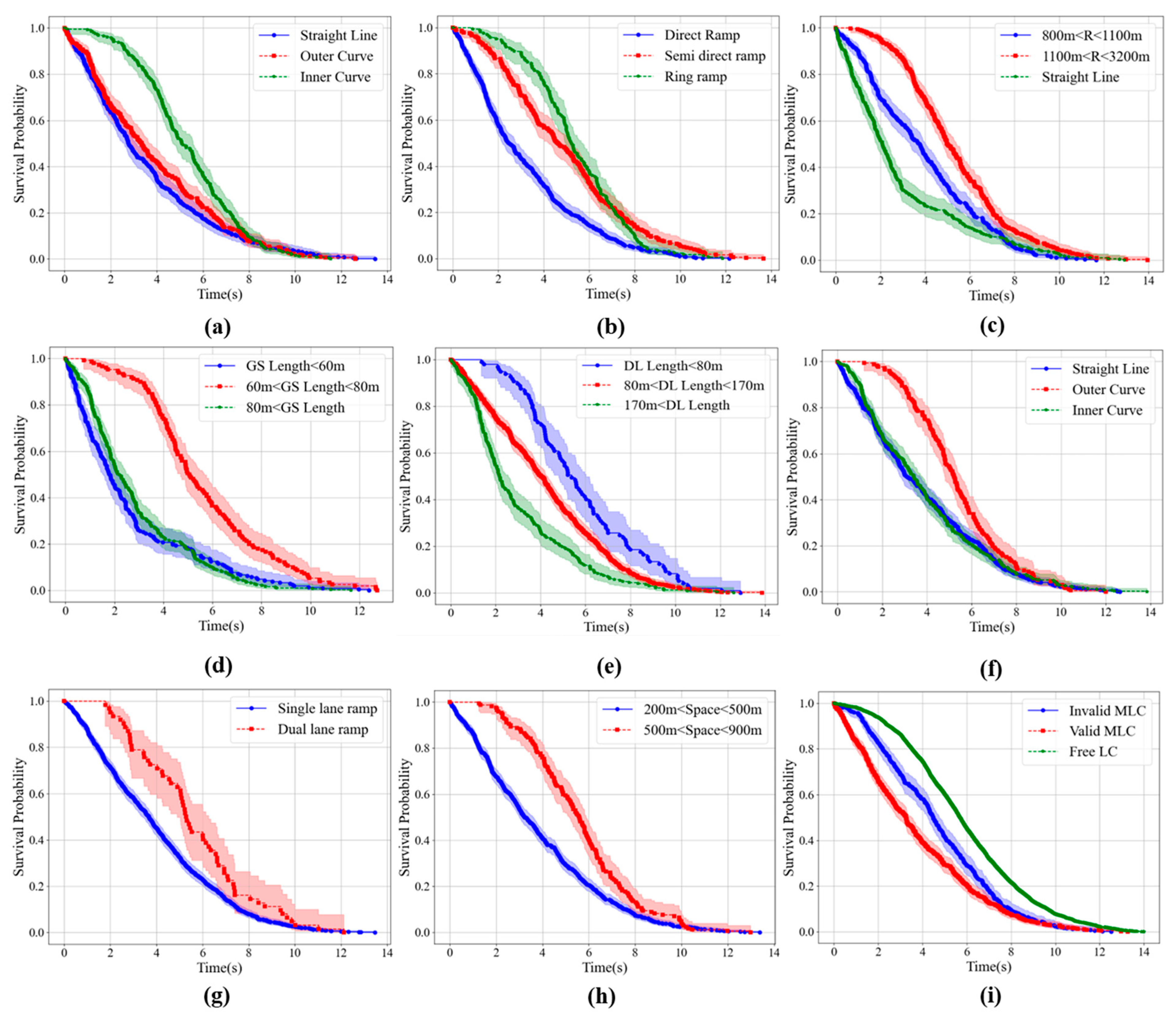
In order to analyze the key influencing factors of MLCs in heavy-duty trucks, after selecting features, we used the Kaplan–Meier non-parametric survival analysis to establish their survival and hazard functions and quantitatively analyzed the distribution characteristics of MLCs under a certain influencing factor (
Figure 8). As shown in the figure, the x-axis represents the duration of lane changing in seconds, and the y-axis represents the cumulative probability curve of MLCs ending within time
. The survival probability at the beginning (0 s) is 1.0, indicating that the lane is starting to shift. However, as time increases, the probability of survival decreases, indicating an increase in the number of events ending (the end of lane changes).
Figure 8i shows that the survival function rapidly decreases within the first 4 s. A sharp decline means that most MLCs are completed in a short period of time. In fact, this period accounted for almost 80% of the total lane change cases. After 8 s, the probability gradually decreases, indicating that over time, MLCs are still surviving less and less. About 20% of lane changes are still active after 8 s, and only 8% of lane changes last for more than 10 s.
The Kaplan–Meier (K–M) method is a statistical method used to estimate the probability of an event occurring within a given time period. We compared different groups by calculating the survival rate at each time point through a curve, as shown in
Figure 8. The survival duration of FLCs is longer than that of MLCs, indicating that MLCs are more urgent and aggressive, while invalid lane changes last longer than valid LCs, indicating that invalid lane changes are exposed to danger for a longer period of time.
Figure 8a shows that the inner side of the curve increases the duration of a LC, but there is no significant difference between the outer side of the curve and the straight line. Compared to direct ramps, semi-direct ramps will increase the LC duration, as shown in
Figure 8b, and the LC duration under circular ramps is the longest, exacerbating the risk.
Figure 8c shows that a small radius can also improve MLCD; for the length of the gradient section,
Figure 8d indicates that an increase in its length will increase the duration, while a decrease in the length of the deceleration lane will exacerbate the unsafe increase in duration, as shown in
Figure 8e. The dual-lane ramp will increase the duration (
Figure 8f).
Figure 8g indicates that an increase in the distance between the merging and diverging nose ends of different interchanges will also increase the MLCD.
Figure 8h shows the effect of the curve direction within the range of 0–800 m before the diversion zone on MLCD, similar to the results in
Figure 8a. Through K–M analysis, it can be found that, for some geometric design indicators, such as the length of the deceleration lane changing within a certain range, it will not have a significant impact on the MLCD. Therefore, it is necessary to apply nonlinear techniques to the extension of the MLC risk function.
4.4. Feature Nonlinear Modeling
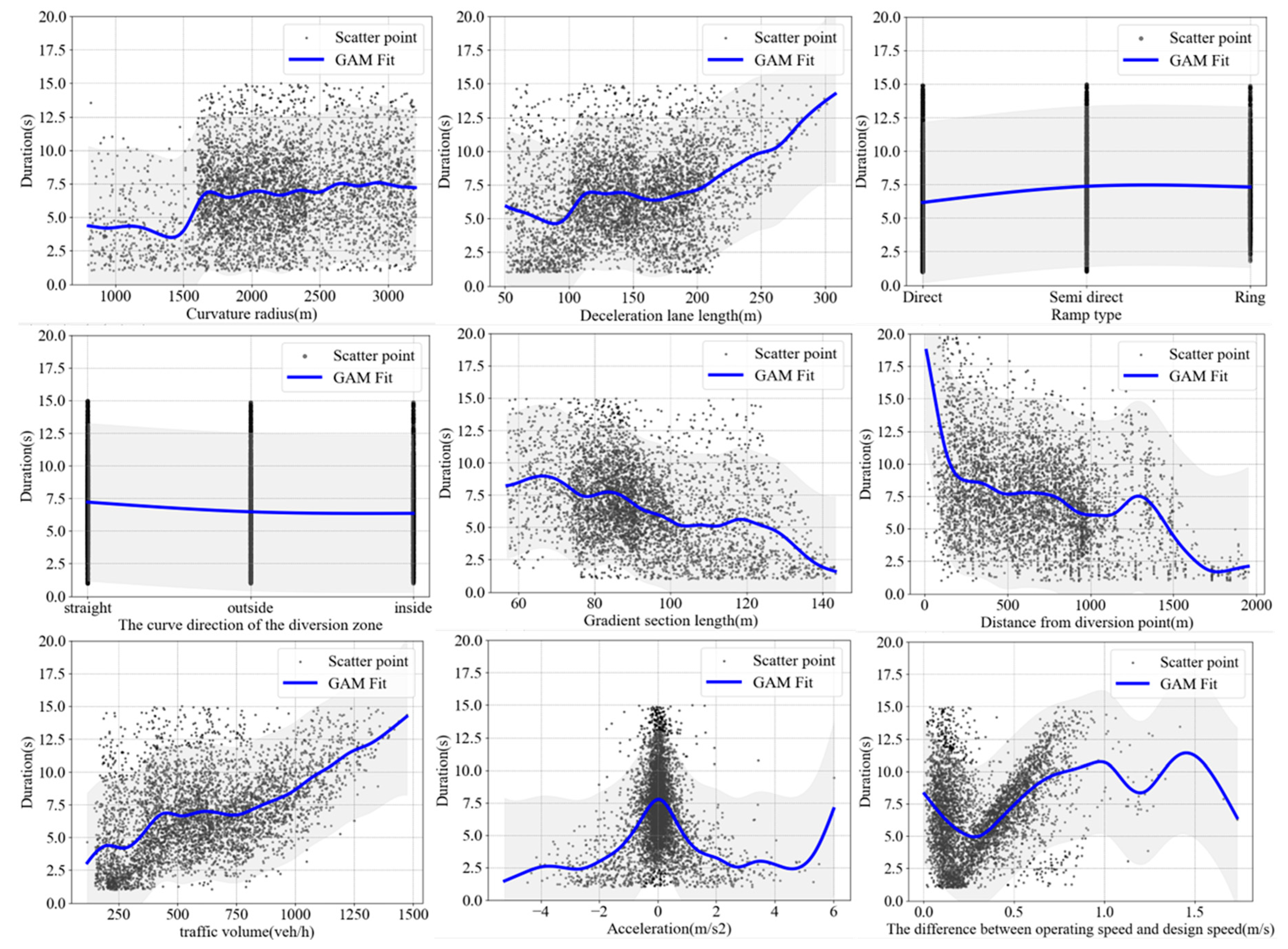
The standard Cox model considered has shortcomings in considering the nonlinear relationships of geometric design elements. By using GAM technology, MLC events are established as nonlinear functions of covariates (
Figure 9). Therefore, it is necessary to consider the smoothing term in the proportional risk model, and we have considered an anti-Gaussian GAM with a smoother. Finding the most suitable smoother requires comparing different options and models with Akaike Information Criterion (AIC) and Bayesian Information Criterion (BIC) measures. It is usually recommended to automatically estimate the smoothing parameters [
28], that is, try the penalty version of the smoother. We compared three commonly used smoothers: cubic spline, P-spline, and B-spline. Regarding cubic splines, the penalty has been modified to shrink towards zero when the smoothing parameter becomes infinite. Specifically, this means that no relationship is correctly identified, i.e., with 0 effective degrees of freedom, rather than modeling with one degree of freedom as in standard cubic splines. For P- and B-splines, the second-order difference of coefficients is penalized to control the smoothness of the spline.
Different smoothing functions lead to different optimizations. Overall, although P-splines and B-splines allow for a direct penalty on coefficients, the cubic spline model has the lowest AIC and BIC, so it should theoretically be preferred, although it does not provide any simple explanation for the shape of nonlinear relationships, such as MLCD and curvature radius.
Although the cubic spline model performs better in metrics, sometimes this highly flexible model does not intuitively reflect the true structure of the data. For example, a cubic spline model is used to model the nonlinear relationship between factors such as vehicle speed and headway and lane changing time. However, in reality, certain parts exhibit sharp changes within a specific range, so it is necessary to balance and consider other smoothers. In addition, for the estimation of smoothing parameters, using automatic estimation is usually a good choice because it can use the features of specific datasets to calibrate the model, reducing subjective bias and improving the model’s generalization ability.
4.5. Model Results
Through K–M non-parametric estimation, it was verified that 2 out of 18 features slightly violated the proportional risk assumption, acceleration and velocity, which are due to the influence of velocity over time, while the remaining variables conform to the assumption. We also used Cox.zph (functional functions) from the survival package in R to examine the hypothesis of Cox models with shared fragility, as shown in
Table 2, and all
p-values, except those at night, were less than 0.06, indicating overall compliance with the PH hypothesis.
In the summary of the Cox Time-Varying Fitter model, the standard error of the covariate coefficients (
Table 2) characterizes how the impact of variables on risk rates changes over time and emphasizes when these effects are significant. Our model is divided into day and night. Specifically, the standard errors of the coefficients for the impact of the number of deceleration lanes and geometric design consistency index on the duration of lane changing are 0.34 and 0.24, respectively, indicating that they have a greater impact on the danger time of MLCs at night. In addition, the standard errors of spatial position, acceleration, and traffic volume are relatively small, all less than 0.1, indicating that the impact of these covariates is constant at different time periods.
The relative impact of factors affecting MLC validity estimated by the Cox-PH regression is shown in
Table 3. Next, we use a shared fragility multiplier with a gamma distribution to correct the Cox PH model. As shown in
Table 3, shared fragility explains the changes in data, while fixed effects cannot explain these changes. Adding shared fragility to drivers can enable each driver to have a different baseline hazard rate, rather than assuming that all drivers share the same baseline hazard level. The distribution of random effects is assumed to be gamma, with an average value of zero. The regression coefficients of the Cox model can explain the risk impact of individual factors on MLCs. Taking X2 as an example, the regression coefficient is 0.001 and the relative risk is 1.001, indicating that when the decision line of sight is reduced by 100 m, the risk rate at the end of the lane change increases by 10%.
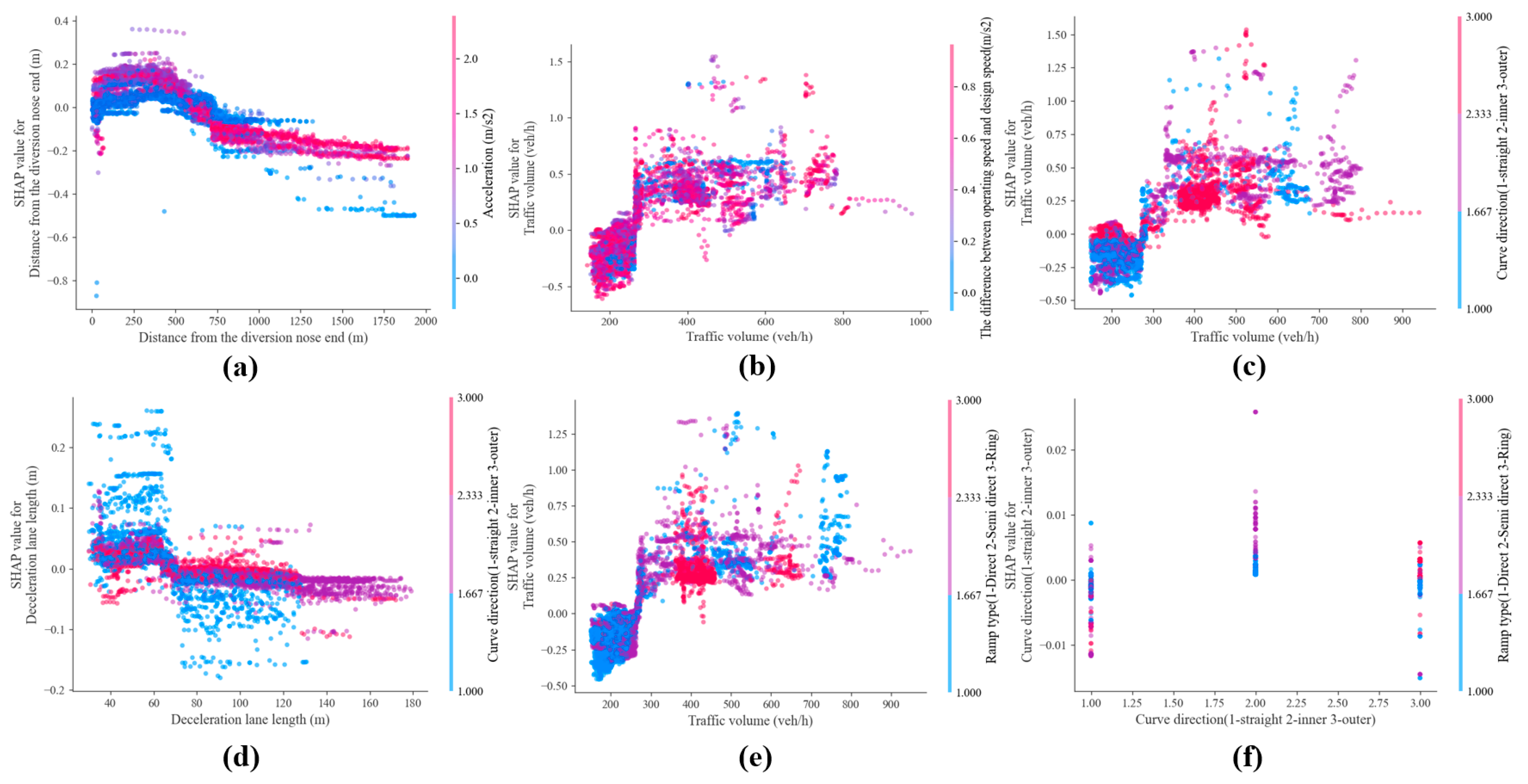
However, the risk coefficients above represent an overall level of impact. To further explain the interaction between covariates, it is necessary to add the SHAP’s dependency graph for analysis. As shown in
Figure 10a, when a driver changes lanes at a distance of 1000 m from the diversion zone, changing lanes at a stable acceleration can reduce the risk, but when a driver changes lanes 500 m away from the diversion area, adopting a fast LC strategy can reduce the risk.
Figure 10b,c,e show that the consistency index of operating speed, the direction of curve curvature, and the type of ramp have significant differences in the impact on MLC under different traffic volumes. The impact of ramp type on MLCs is attributed to vehicles traveling on semi-direct and circular ramps slowing down at the front of the ramp, especially on circular ramps. As traffic volume increases, this will increase the workload of drivers to varying degrees. The regulations on the length of deceleration lanes in the “Design Guidelines for Interchanges in China” are related to the design speed. However, the results in
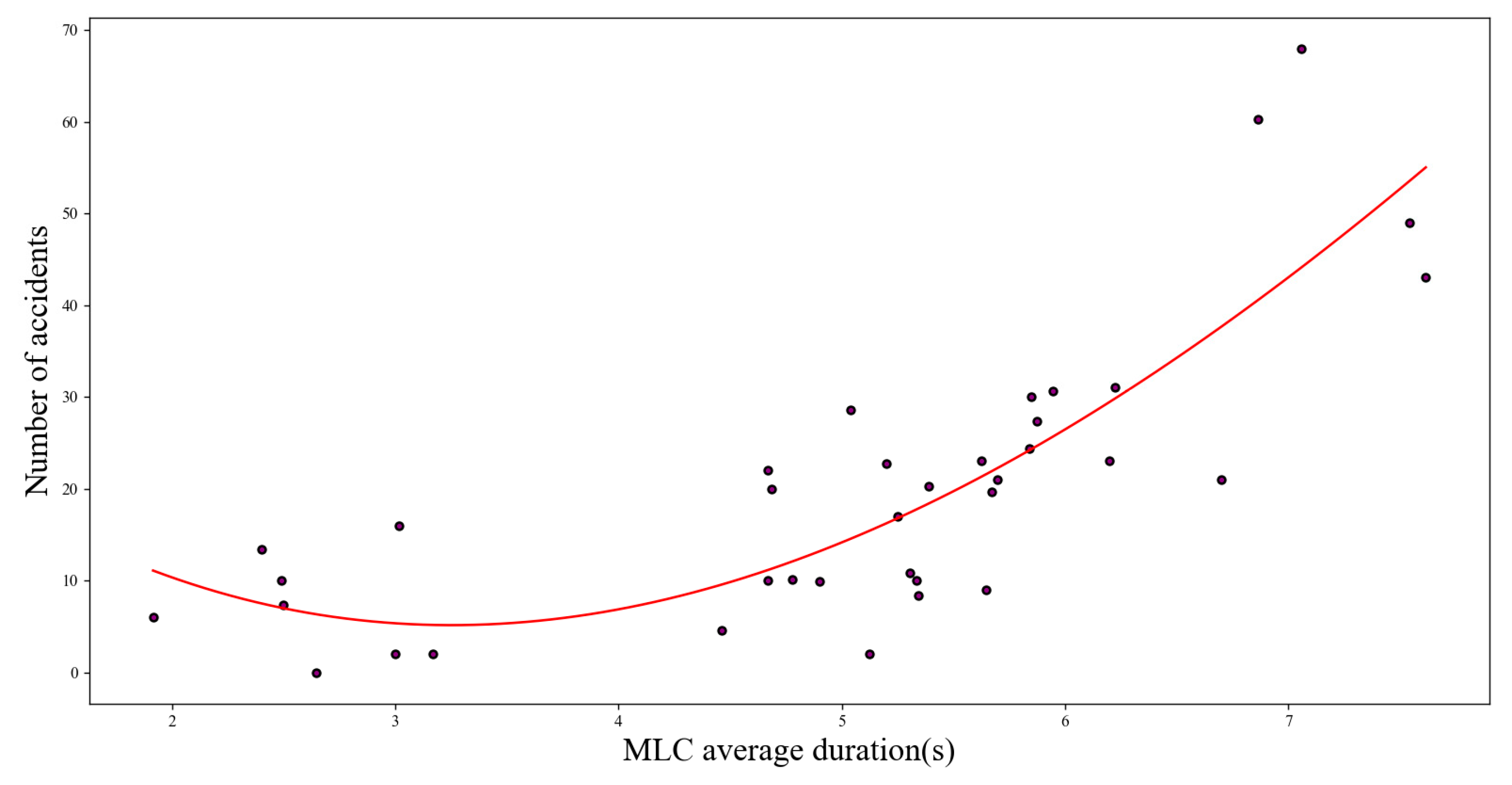
Figure 10d indicate that it is also related to the bending direction of the circular curve. In addition, we also conducted a statistical analysis on the relationship between the number of traffic accidents at each interchange within 3 years and the average MLCD. As shown in
Figure 11, this relationship shows a concave curve, with fewer accidents occurring within an average lane changing time of 5 s. However, the growth rate of accidents sharply increased after 5 s, indicating that the longer the exposure time for lane changing, the more likely it is to lead to accidents, which is consistent with the existing research [
21]. These results indicate that the geometric elements of interchanges have a significant impact on MLCs, and these analyses emphasize that the geometric design of interchanges should not only consider the impact on the speed of small vehicles, but also the lane changing behavior of heavy trucks, as MLCs have caused a significant proportion of serious traffic accidents.
4.6. Model Evaluation and Comparison Results
We chose the consistency index, partial AIC, and logarithmic likelihood ratio test to evaluate the model. The consistency index is usually between 0 and 1, where 1 represents complete consistency and 0.5 represents random guessing. The higher the consistency index, the better the model can distinguish the survival period. Partial AIC is used to compare the effects of adding or removing variables in Cox models, and a decrease in partial AIC indicates that the fit of the model is improved by adding or removing variables. The log likelihood ratio test is used to compare two nested models. If the
p-value of the log likelihood ratio test is small, the null hypothesis can be rejected, indicating significant differences between the models and the added or removed variables having an impact on the model fitting. As shown in
Table 4, there are some differences between the standard Cox PH model and the improved model. Specifically, the factor indicators in the time-varying Cox model using GAM technology are higher than those in the standard model, with a consistency index of 0.85 and a log likelihood ratio test of 196.20. In the standard Cox model, the consistency index is 0.8 and the log likelihood ratio test is 377.15. Unlike this result, after adding the shared fragility parameter, the consistency index of the two models increased to 0.9, but the logarithmic likelihood ratio test increased to 964.63. The improvement of the consistency index indicates that the model’s ability to rank or distinguish individual risks is enhanced, which means that the prediction accuracy of the model in practical applications is improved, although the decrease in the logarithmic likelihood ratio test reflects some of the risk of overfitting. In addition, there were 17 important variables in the models before and after adding shared fragility, and the fragility period was significant (
p-value < 0.001). Therefore, the fragility shared by the drivers improves the accuracy of the Cox model. However, if only the shared fragility of the interchanges is increased, all variables related to road geometry design are excluded, that is, the driver’s MLC on any interchange is related to the spatial location, nighttime speed, traffic flow time variables, and the acceleration of its own state. After excluding variables, the consistency index (0.77) significantly decreased, as shown in
Table 4. In addition, if both the random effects of the drivers and road segments are considered, the model is only related to spatial position and acceleration. This also indicates that the Cox model introduces the randomness of drivers to capture the variability of unconsidered explanatory data and emphasizes the important impact of road geometry design on MLC behavior.
In addition, due to the widespread application of AFT models in lane changing modeling, we compared the standard AFT model with the Cox model. Unlike Cox, the AFT model assumes that covariates have an accelerating or slowing effect on survival time and survival time follows a specific distribution. As shown in
Table 4, the evaluation of the AFT model is lower than that of the standard Cox model. We determined that the AFT model made assumptions about the distribution of survival time (Weibull distribution). The advantage of this assumption is that it can directly model the duration of FLC on general road sections, but the actual data of MLCs in interchange areas may not fully conform to these distributions. However, the Cox model did not make specific assumptions about the distribution of the MLCD and can be extended to consider the temporal dependence of variables, making it more suitable for modeling MLCD in complex interchange scenarios.
Next, we use a shared fragility multiplier with Weibull distribution to correct the Cox PH model. There is almost no difference between the shared fragility models of gamma and Weibull distributions. The concordance of the goodness of fit measurement is 0.90 and the log likelihood ratio test is 942.46. There are 17 significant variables that are similar to the results of the shared fragility model of the gamma distribution, but there is a slight difference in the risk ratio. Overall, this sensitivity analysis indicates that these findings are stable for distribution types.
5. Discussion
5.1. Main Findings and Theoretical Significance
In order to analyze the intrinsic safety of heavy trucks operating at interchanges, we used large-scale, full time-domain, and high-precision floating freight vehicle data to analyze the mandatory lane changing behaviors of the main line in front of the interchange diversion area. We found that the MLCD for heavy-duty trucks is 0.5~1 s shorter than FLC, and the variance of MLCD is higher. Compared with the MLCD of small cars previously studied, heavy-duty trucks take about 0.6 s longer than small cars. Interestingly, invalid MLCDs are concentrated within 5 s, which is about 3 s longer than valid MLCs. From the position of changing lanes, MLCs are mainly distributed around 170 m to 800 m in front of the diversion zone. In addition, the relationship between accident frequency and MLCD shows a concave curve, with fewer accidents occurring within an average lane changing time of 5 s. However, the growth rate of accidents sharply increased after 5 s, indicating that the longer the exposure time for lane changing, the more likely it is to lead to high-frequency accidents. The model we have established indicates that the distance of vehicles reaching the diversion point, consistency in geometric design, traffic volume, day and night, direction of bending of a circular curve, ramp type, length of deceleration lane, radius of road circular curve, and number of deceleration lanes have a significant impact on the risk of heavy truck MLCs, and the degree of these effects can be expressed by the relative risk value of the model. Importantly, these impacts are nonlinear and have diurnal differences. In addition, the SHAP tool indicates that there are complex interactions among various factors, among which the consistency index of operating speed, the direction of bending of a circular curve, and ramp type under different traffic volumes have varying degrees of impact on the duration of MLCs. This difference is also reflected in the relationship between the distance and speed of vehicles reaching the diversion point, as well as the relationship between the direction of bending of a circular curve and the type of ramp and the length of the deceleration lane.
We provide a full time-domain trajectory big data-driven MLCD model for heavy-duty trucks at interchanges. We hope to provide a theoretical basis for improving the consistency between the design of interchanges and the lane changing characteristics of heavy-duty trucks fundamentally. We improved the standard Cox model by first using the GAM to represent the relationship between covariates and MLCD as a nonlinear risk function. The AIC index indicates that the cubic spline curve is optimal in reflecting the nonlinear characteristics of the geometric elements of interchanges. In addition, we added a time-related module to analyze the time effects of covariates, and the standard deviation of the coefficients of these covariates reflects the diurnal differences in the impact of covariates. Among them, the number of deceleration lanes and the consistency index of operating speed have a significant difference between day and night in the impact on MLCs, while the impact of the remaining elements remains basically unchanged at different time periods. In addition, we also modify the model by sharing fragility parameters to consider the heterogeneity of lane changing among different drivers. In summary, we used a time-varying Cox model with combined GAM techniques, with a consistency index of 0.90 and a log likelihood ratio test of 964.63. This has a higher consistency index than the standard model, indicating a significant enhancement in the model’s ability to rank or distinguish individual risks. This means that the prediction accuracy of the model has been improved in practical applications, although the decrease in the logarithmic likelihood ratio test reflects some overfitting risks.
5.2. Practical Significance
Understanding the effective probability of MLCs in interchange areas and the factors influencing these events are important focus areas of concern for researchers and practitioners, as ineffective lane changes have caused a large number of serious traffic accidents in interchange areas. The feature set of important factors used in our model is now relatively easy to obtain and is usually more accurate in most interchange areas. Our research findings focus on heavy-duty trucks and consider the most adverse effects of various factors on MLCs. We hope that this probability assessment will improve the quality of road geometry design. However, the provisions on the length of deceleration lanes in the Chinese Interchange Design Guidelines are only based on considerations of the operating speed of small vehicles. However, the data suggest that this consideration may not necessarily reduce the risk of MLCs. When the direction of the curve is on the inside, the risk of a MLC in a 35–70 m-long deceleration lane is lower; when the bending direction of the curve is on the outside, the risk of a MLC is lower for deceleration lanes with a length greater than 80 m. The degree of influence of geometric elements on different traffic volumes varies. In summary, our research provides insights into the combinatorial and diverse aspects of geometric design, emphasizing the importance of considering MLCs. In addition, with the advancement of research on autonomous vehicles, the development trend of linear design optimization has gradually changed to multi-objective optimization, and the optimization goal has transitioned from economic cost to safety and ecological cost. In the interchange area, the research results and methods of this article can guide the reduction of the risk of lane changing events through reasonable design, thereby reducing energy consumption and improving overall transportation efficiency, such as optimizing the management and scheduling efficiency of autonomous driving fleets. In addition, the method proposed in this paper can reduce the lane change demand of autonomous vehicles in these areas, reduce accident risk, and improve traffic smoothness.
Ultimately, it is worth pointing out the limitations of our research. Although our data have a wide range and full time characteristics, they have a lower sampling frequency compared to NGSIM and highD. In addition, we did not consider factors such as the location of traffic signs, driver-specific factors, and differences in traffic conditions around specific MLCs. Although this has little impact on the study of variables such as geometric design, it can be considered to improve the accuracy of the model in the future. In addition, we also lack a comparison of the MLC behavior of small cars under the same interchange conditions. In the future, we will collect more high-frequency floating vehicle data on interchange types to analyze MLC characteristics under more factors.


