Connectedness of Carbon Price and Energy Price under Shocks: A Study Based on Positive and Negative Price Volatility

Abstract

We calculate both positive and negative price volatilities based on Realized Semi-variance (RS) in major economies’ carbon and energy markets with daily data from 1 July 2013 to 31 May 2023. Subsequently, we construct a network using the Elastic-Net-VAR model to analyze the contagion of price volatilities and examine how shocks affect the connectedness between these markets’ price volatilities using Local Projection. The following findings are presented: (1) There exists a robust correlation between carbon price volatilities and energy price volatilities, with time-varying overall network connectedness ranging from 21.54% to 83.34%. (2) Carbon markets primarily act as recipients of price volatilities, while energy markets serve as initiators. (3) The spillover effects and inflow of negative price volatilities are more pronounced compared to those of positive price volatilities. This is attributed to the fact that declining prices often indicate a market downturn, leading to the easy dissemination of adverse news across interconnected markets. Concurrently, increasing fragility diminishes its resilience against risks. (4) Shocks have a significant influence on the connectedness between carbon prices and energy prices, with different mechanisms at play under different shocks. The COVID-19 pandemic has increased the connectedness between carbon markets and energy markets primarily through common exposure mechanisms. Conversely, geopolitical risks reduce network connectedness by decreasing price complementarity.

1. Introduction

Climate, as a crucial element of the living environment, not only impacts humans’ living conditions but also significantly influences the long-term sustainability of economic development. Since the advent of the Industrial Revolution, greenhouse gas emissions have escalated rapidly. This surge in emissions has propelled global warming to become a formidable global threat, prompting an increasing number of countries to proclaim their commitment to carbon neutrality. The 2015 Paris Agreement outlined an ambitious objective of achieving carbon neutrality worldwide by the latter half of this century. Carbon neutrality has unequivocally emerged as a pivotal component and developmental objective within the realm of global emission reduction efforts. In theory, preserving environmentally sustainable and low-carbon growth lies in curbing greenhouse gas emissions and decelerating the progression of the greenhouse effect. Reducing reliance on fossil fuels stands at the core of managing greenhouse gas emissions.

The EU Emissions Trading System (ETS), a carbon trading mechanism established in accordance with EU Directive (2003/87/EC) (See https://eur-lex.europa.eu/legal-content/EN/TXT/PDF/?uri=CELEX:02003L0087-20180408 (accessed on 7 May 2024)), originated in 2005. Greenhouse gases included in the EU carbon emission system include carbon dioxide (CO₂), nitrous oxide (N₂O) and perfluorinated compounds (PFCs). After that, the international carbon emission trading market has experienced rapid expansion. To achieve the goals of the Paris Agreement, the European Commission published the European Great Deal, a new growth strategy document, on 11 December 2019. In June 2023, the Member States of the European Parliament and the Council of the European Union formally adopted the EU ETS proposal, making it a regulation. As financial intermediaries and international politics become increasingly involved, the complexity and volatility of carbon markets have also grown. Furthermore, the rapid development of the carbon trading market has led to its close connection with the energy market. Carbon price volatilities are highly pro-economic cyclical [1,2,3]. Through the lens of the global value chain [4], a country’s carbon emissions are influenced by the spillover and feedback effects within its supply chain, intensifying the interdependence between the international energy and carbon markets. Simultaneously, policies related to carbon market development can impact the supply and demand dynamics as well as price volatilities of the energy market, exerting a profound influence on the energy industry.

Illustrated in Figure 1 are certain regular patterns observed in the volatilities of the carbon market and the energy market. Particularly noteworthy are the significant market swings coinciding with geopolitical events, such as the 2018 US–Iran crisis, the 2022 Russia–Ukraine conflict, as well as the detrimental effects of the COVID-19 outbreak in 2020. These observations suggest the presence of risk resonance effects between the energy and carbon markets, with price movements susceptible to extreme shocks.

Note: In the graph, “Volatility of Carbon Price” represents the average volatility of carbon prices in Europe, China, and America, while “Volatility of Energy Price” represents the average volatility of fossil energy prices, encompassing coal, crude oil, and natural gas. The Carbon Price data are derived from the Aggregate Real Carbon Price (Europe/China/America) available in the Bloomberg database, provided by Monash University & C2Zero. The Energy Price data are sourced from the Wind database, comprising the futures closing prices of IPE Brent Crude Oil, IPE UK Natural Gas, and IPE Rotterdam Coal active contracts. To estimate the volatility of each price, we employed the GJR-GARCH model introduced by Glosten et al. (1993) [5].

Indeed, the prices and risks in the carbon and energy markets are interconnected. External shocks or policy changes have the potential to transmit and amplify risks within and across both markets. The trading nature of carbon markets and energy markets implies that when the risks in these markets become excessively high, they can spillover into the other part of the economy, such as the production activities of enterprises. The interlinkages between the energy and carbon markets create a pathway for risk contagion, impacting the sustainability of the economy. As a result, studying the correlation mechanism between these markets becomes imperative since the negative externalities ultimately affect the production activities of enterprises. Understanding this correlation mechanism can help uncover potential transmission channels and devise appropriate risk management strategies to mitigate risks and promote a sustainable economy.

However, is the connectedness of carbon price and energy price robust and continuous? What are the temporal characteristics of the connectedness? What are the characteristics of the connectedness of rising and falling prices in various markets over different periods? What mechanism lied behind the connectedness? Do shocks such as geopolitical risks and public health events affect the correlation between carbon and energy prices? These are all important and worthy of discussion.

Based on the above questions, we use the Realized Semi-variance (RS) method proposed by Barndorff-Nielsen et al. (2008) [6]. We examined the price volatilities of carbon prices and energy prices and their connectedness. The RS method allows for the exploration of spillover relationships between markets in terms of positive price volatility and negative price volatility. It has been applied to analyze cross-sector volatility contagion in the stock market [7], the impact of geopolitical risk uncertainty on oil futures price volatility [8], the positive and negative effects of macroeconomic uncertainty on asset prices [9], and the asymmetric spillover effect between the oil market and the stock market [10].

Furthermore, following the research framework of Diebold and Yilmaz (2014) [11], we construct the connectedness network of carbon markets and energy markets based on the generalized prediction error variance decomposition method of the Elastic-net-VAR model [12]. This model has been utilized to investigate the spillover of economic policy uncertainty to the electricity market [13] and the volatility spillover between emerging stock markets and cryptocurrencies [14]. In comparison to other methods, this approach can capture the elastic correlation between markets. Additionally, extreme events such as geopolitics and public health events may also influence the price volatilities of carbon and energy. We further utilize local projection [15] to investigate the impact of extreme events on the price fluctuations of carbon and energy markets.

The main objectives of this study are as follows: First, we hope to comprehensively explore the correlation and characteristics of carbon prices and energy prices and analyze their time-dimensional characteristics to further investigate the price correlation law between carbon markets and energy markets. This is conducive to the reasonable formation of carbon market prices. Second, we hope to explore the mechanism behind the correlation between carbon prices and energy prices by measuring the impact of shocks on correlations. On this basis, it provides reasonable suggestions for investors’ risk asset portfolios.

The main findings are as follows. First, we find that there is a strong correlation between major carbon prices and energy prices, and there is a significant difference between positive price fluctuation correlation and negative price fluctuation correlation. This provides a basis for investors to include carbon market products in their portfolios. Second, for different shocks, the correlations between carbon markets and energy markets respond to shocks in different directions, and the response directions of each type of price correlation to shocks are also heterogeneous. This provides a basis for investors to dynamically adjust their portfolios according to shocks.

The remaining part of this paper is arranged as follows: the second part is a literature review; the third part is a pre-analysis of the mechanism of connectedness between carbon price and energy price; the fourth part is the method and data used in this paper; the fifth part is the main empirical results and analysis; the sixth section is the discussion. The research framework of this paper is shown in Figure 2.

2. Literature Review

Existing studies have confirmed the connectedness between carbon market and energy market price and volatility in various ways and sorted out the correlation mechanism of the carbon market and energy market accordingly [16,17,18,19,20,21,22]. Some studies believe that the relationship between the two is mainly the top-down transmission of risk. That is, the energy market, as the upstream of the industrial chain, is transmitted to the downstream carbon market. Energy prices can provide useful help in carbon price projections. Nazifi and Milunovich (2010) [23] found a short-term link between EU ETS prices and coal, crude oil, gas and electricity prices. They argue that carbon markets do not directly affect energy market prices but can effectively change the efficiency of energy use. Keppler and Mansanet-Bataller (2010) [16] analyzed the interaction of carbon prices, the electricity market and natural gas prices with EU ETS prices in stages. Aatola et al. (2013) [18] empirically tested the formation mechanism of the EU ETS price and found that it was significantly correlated with energy prices, especially German electricity prices, natural gas prices and coal prices. Zhang and Sun (2016) [19] paid attention to the volatility spillover of the carbon price and energy price and analyzed the volatility spillover between markets respectively. They found there is the strongest correlation between the coal market and the carbon market. Ji et al. (2018) [21] used the time series method to study the information flow and connection between the carbon market and the energy market, proving the important impact of crude oil prices on carbon price changes. Zhu et al. (2017) [20] used bivariate empirical mode decomposition (BEMD) and linear and non-linear Granger causality tests to explore the interaction between carbon prices and electricity prices in different periods. Batten et al. (2021) [22] argue that in addition to energy prices, unexpected climate change will also affect carbon prices. The above studies show that there is an important link between carbon prices and energy prices.

Some studies have also focused on carbon and energy prices in the context of financial markets or macroeconomics. They introduce macro factors into their research by building network models of carbon, energy and financial markets or other macro variables. These studies pay more attention to the formation of carbon price and energy price and their underlying influencing factors. In addition, some studies have focused on risk contagion between carbon and energy markets at the country level. This is mainly because the energy price is greatly affected by international factors, while the influencing factors of carbon price have certain country heterogeneity. Jin et al. (2023) [24] constructed dynamic network spillover models of energy risk, climate risk and geopolitical risk and found strong network connectivity. Further, they found that the risk spillover among the three is higher in the state of high volatility frequency, and geopolitical events will drive the increase of network correlation. Liu et al. (2023) [25] Construct a two-tier spillover network of the electricity market, traditional energy market and carbon market in European countries to explore the impact of climate risk on network structure and nodes. They found that there are two-way spillovers between markets and that extreme events such as the Russia-Ukraine conflict can have an impact on network structure. Meng et al. (2023) [26] constructed a time-varying global spillover network to study the risk spillover effects of carbon prices and shipping energy prices and found that traditional Marine energy prices had a greater impact on carbon prices. Naeem and Arfaoui (2023) [27] use CAViaR and TVP-VAR models to investigate the relationship between extreme downside risks in electricity, clean and conventional energy and carbon markets. They found that in cases of extreme downside risk, correlations between markets increased. Wang et al. (2023) [28] used the quantile spillover index to construct the global risk spillover network of climate uncertainty, energy market, carbon market and green bond and argued that in the state of extremely high risk, the correlation between various markets is enhanced, and extreme events have a significant impact on network connectivity. Hoque et al. (2023) [29] constructed a risk spillover network of the volatility of carbon, climate and energy futures and found that it had a short-term correlation and was affected by extreme events. Naeem et al. (2020) [30] used spillover networks to investigate the correlation mechanism between electricity, carbon and clean energy markets and oil price demand and supply shocks and found that the impact of events such as the global financial crisis and the shale revolution would have a greater impact on network connectedness.

To measure the spillover effects between energy prices and carbon prices, previous studies have used different methods. Previous studies were based on the combination of DCC-GARCH and BEKK-GARCH [19], total spillover index and directional spillover index based on vector autoregressive (VAR) model [11], CoVaR combined with GARCH method [31], Copula method combined with CoVaR method [32], EGARCH model [33] and MS-DCC-GARCH model [34] to study the connectedness between different energy market prices and carbon prices.

Through the literature review, we found that with the rapid popularization of carbon trading in the world, scholars have conducted more studies on the interaction between carbon prices and energy prices in the international market. At the same time, there are few studies on the risk spillover of the energy market and carbon market from the perspective of positive price volatilities and negative price volatilities. Compared with the international carbon markets, China’s carbon market started relatively late, so there is literature that includes China’s carbon market in the research scope. As the second largest economy (China has been the second-largest economy for years. According to a 2011 report by NPR and the Wall Street Journal, China’s GDP surpassed Japan’s in 2010 to become the world’s second-largest economy. In the years since, China has been second only to the United States in terms of GDP. For details, see https://www.npr.org/sections/thetwo-way/2011/02/14/133747019/confirmed-china-has-worlds-no-2-economy-passes-japan (accessed on 6 May 2024)), China has set up carbon emission trading pilot projects in Shenzhen, Guangdong, Beijing, Shanghai, Hubei, Tianjin, Chongqing and Fujian to implement its plan to curb greenhouse gas emissions. On 16 July 2021, China’s national carbon market officially launched trading, becoming the world’s largest market covering greenhouse gas emissions. In addition, as the world’s second-largest economy, China’s carbon trading behavior may have an important impact on carbon prices and trading mechanisms. Therefore, it is necessary to include China’s carbon market in the scope of research. Based on the existing research on the EU carbon market and the US carbon market, this paper further includes the Chinese carbon market to explore the price connectedness between markets. This paper can effectively measure the spillover effect between the energy markets and the carbon markets and help to deeply investigate the mechanism of price correlation between the carbon markets and the energy markets. This is of great significance for further promoting the risk prevention of carbon markets and energy markets and promoting the stable operation of the carbon trading system.

We present three main contributions. First, for research methods, we innovatively apply the semi-variance decomposition method to the construction of the connectedness network between carbon market price and energy market price. We believe that the method of semi-variance decomposition, which divides the price volatilities into positive and negative volatilities, is of great significance in exploring the different directions of price changes caused by different extreme shocks. By comprehensively characterizing the spillover effects within and between various types of volatilities, we accurately grasp the risk resonance and contagion characteristics between carbon markets and energy markets. Both positive volatility (extreme increase in price) and negative volatility (extreme decrease in price) may lead to an increase in risk, so it is of great practical significance to discuss them separately. In terms of research ideas, we provide a new way to examine abrupt changes in the connectedness network, which allows us to comprehensively analyze the connectedness network between carbon prices and energy prices. Based on the global correlation perspective of carbon and energy, we construct a connectedness network containing positive and negative price volatilities and adopt the Elastic-Net method to solve the estimation problem of the high latitude VAR model. Further, we use the local projection method to explore the impact of major shocks on network structure and risk contagion. The application of the local projection method allows us to accurately identify the degree and trend of network structure changes. From a practical point of view, we provide important evidence for the transmission of carbon trading price risk between countries and the risk transmission from the energy market to the carbon trading market, which has important reference significance for various countries, especially those countries whose carbon market is just starting. By introducing the relative spillover index, we explore the asymmetric characteristics of directional spillover of positive and negative volatility in each market and the heterogeneity of impact direction on different markets. Our research shows that more developed carbon markets are more vulnerable to risk but also more resistant to it. Therefore, in the process of developing the carbon market, it is very important to evaluate the development degree of the carbon market and choose the policy of blocking the risk.

The significance of our study lies in the following aspects: For production enterprises, gaining insight into the connectedness of carbon price and energy price serves as a basis for optimizing energy structures and enhancing overall production efficiency. For the carbon emissions trading market, comprehending the connectedness of carbon price and energy price and possible mechanisms aids in assessing whether carbon prices accurately reflect changes in market fundamentals. For investors, analyzing the interconnection mechanism between the carbon price and the energy price provides valuable information for effective asset allocation and portfolio optimization. Lastly, for governments, a thorough understanding of the connectedness of carbon price and energy price and possible mechanisms contributes to the formulation of robust and effective environmental regulations and policies.

3. Pre-Analysis of the Connectedness Mechanism

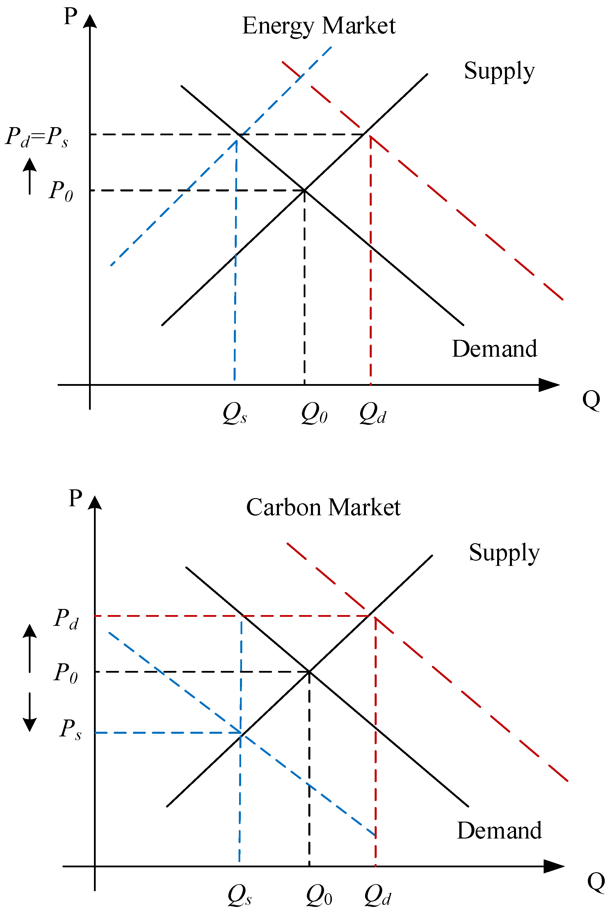
3.1. Supply and Demand Mechanism

According to the literature review, the connectedness of carbon prices and energy prices does exist. In this section, we further examine the possible underlying mechanisms of connectedness. We first discuss the connect mechanism between carbon price and energy price from the basic supply and demand mechanism. Figure 3 illustrates the supply–demand mechanism of the connection between the carbon price and energy price. Changes in energy prices can be attributed to two factors: supply-side drivers and demand-side drivers. In the case of increasing energy prices, either a decrease in energy supply (resulting in a leftward shift of the energy supply curve) or an increase in energy demand (leading to a rightward shift of the energy demand curve) can contribute to an upward movement in the equilibrium price of energy. The quantity at which equilibrium is reached determines the demand for carbon emission permits.

In the event of a decrease in energy supply leading to an increase in energy prices, there is a corresponding decrease in the equilibrium quantity of energy. Consequently, when there is a decline in demand for carbon emission permits, it causes a leftward shift in the demand curve for these permits. Assuming that the supply curve remains unchanged, this results in a decrease in the equilibrium price of the carbon market. Therefore, it can be observed that there exists a negative correlation between energy prices and carbon prices when changes are driven by fluctuations on the energy supply side.

In the case of higher energy prices driven by increased energy demand, there is an upward shift in the equilibrium quantity of energy. Consequently, an increase in demand for carbon emission permits leads to a rightward shift in the demand curve of carbon emission permits, resulting in an increase in the equilibrium price of the carbon market when the supply curve remains unchanged. Thus, a positive correlation exists between changes in energy price and carbon price when driven by changes on the energy demand side.

3.2. Common Risk Exposure

The synchronized movements of carbon and energy prices may be due to a common risk exposure mechanism. The mechanism of common risk exposure (Fleming et al., 1998) [35] primarily focuses on the connection between markets resulting from shared external shocks. In the event of an external shock, particularly a significant one such as the COVID-19 pandemic, it exposes the economic system to comparable risks. Both carbon markets and energy markets are susceptible to identical sources of risk and are interconnected through common risk factors.

3.3. Price Elasticity Analysis

To further explain the rationality and necessity of our research on price performance, we analyze this problem from the perspective of supply price elasticity. The reason is that our analysis of how carbon and energy markets behave under shocks is more based on demand-side shocks (e.g., COVID-19 shocks and geopolitical risk shocks). This further confirms the rationality of the supply and demand mechanism and the common risk exposure mechanism mentioned above. In this part, we estimate the supply price elasticity of the carbon market and make a comparative analysis based on the calculation of energy price elasticity in existing literature (Kilian, 2022) [36]. Similar to energy markets, both supply and demand in carbon markets are endogenous variables, so we cannot estimate elasticity using a direct regression of trading volume to price. Therefore, with reference to Gabaix and Koijen (2021) [37], we adopted the cutting-edge granular instrumental variable method and took the EU emission trading rights as an example to estimate the supply price elasticity of carbon allowances. The specific calculation method is as follows:

$$∆P_t=\gamma {∆Z}_t+{\epsilon }_t$$

(1)

where $∆P_t$ is the rate of change in EU carbon price, ${∆Z}_t$is the structural carbon demand particle tool variable, and the regression coefficient $\gamma$ is the supply price elasticity of the carbon market. The process of constructing ${∆Z}_t$ is as follows. First, a weighted average of carbon consumption is carried out, where the weight used is the proportion of the GDP of the countries in the EU to the total GDP of the EU.

$$S_{i,t}=\frac{{GDP}_{i,t}}{\sum {GDP}_{i,t}}$$

(2)

Here, we can obtain the weighted carbon emission as follows:

$$q_t^S=\sum S_{i,t}\times q_{i,t}$$

(3)

where $q_{i,t}$ is the carbon emission of EU member State i during the period t. Further, we define the arithmetically average carbon emissions of each country as follows:

$$q_t^E=\frac{1}{i}\sum q_{i,t}$$

(4)

Further, we can construct an instrumental variable for measuring the supply price elasticity of carbon emissions:

$$Z_t=q_t^s-q_t^E$$

(5)

$Z_t$, as a proxy variable of carbon consumption, has both externality and correlation. It is reasonable and correct to calculate the elasticity of the carbon market by excluding the influence of common shocks and retaining only the influence of individual shocks. In the calculation process, the carbon emission data comes from the CEADS (Carbon Emission Accounts and Datasets) (https://www.ceads.net/ (accessed on 8 June 2024)) database, and the GDP data of each country comes from WIND. Due to the availability of carbon emission data, we have included the EU countries as a whole (others), excluding the UK (the United Kingdom left the European Union on 31 January 2020, local time, but it is still having an impact in Europe. And because the database used in this paper is calculated for EU carbon emissions and the UK as a whole, the time span covers data up to 31 December 2020. In order to ensure the completeness and rationality of the data, the United Kingdom is included in the calculation), France, Italy, Germany, and Spain. In addition, due to the high frequency of carbon emission data and the absence of daily frequency data, we reduced the frequency of carbon emission data used in regression to weekly frequency to take the weekly average. The GDP frequency used for weighting is the quarterly frequency. The data range is from 1 January 2019 to 31 December 2023. Descriptive statistics of the basic data used in the calculation are shown in

Table 1. Descriptive statistics of date used in calculating Price elasticity of supply.

Variable	Obs	Mean	Std. Dev.	Min	Max
GDP_EU27 (Millions of euros)	116	269,2603.00	697,915.60	1,552,569.00	4,313,506.00
GPD_Italy (Millions of euros)	116	381,641.90	69,262.39	213,695.30	527,492.20
GDP_France (Millions of euros)	116	484,117.90	107,143.50	301,164.00	712,521.80
GDP_Spain (Millions of euros)	116	239,373.10	65,905.82	112,945.80	375,161.00
GDP_Germany (Millions of euros)	116	673,202.00	152,719.40	485,577.20	1,053,040.00
GDP_UK (Millions of euros)	116	402,398.10	124,626.00	207,126.00	678,310.00
Carbon emission_EU27 and England(kton)	1947	8.23	1.56	4.46	12.28
Carbon emission_France(kton)	1947	0.78	0.19	0.29	1.25
Carbon emission_Germany(kton)	1947	1.73	0.46	0.77	3.01
Carbon emission_Italy(kton)	1947	0.84	0.18	0.39	1.28
Carbon emission_Spain(kton)	1947	0.64	0.12	0.29	0.98
Carbon emission_UK(kton)	1947	0.92	0.18	0.45	1.46
Carbon emission_Others (kton)	1947	3.32	0.58	1.89	4.96

below.

Our regression calculation results are shown in the table below:

There is an interesting result in

Table 2. Calculation results of price elasticity of supply.

Variables	$∆{\mathit{P}}_{\mathit{t}}$
${∆Z}_t$	0.0527 ***
	(0.0198)
Constant	−0.345 **
	(0.137)
Observations	260
R-squared	0.021
Robust standard errors in parentheses

*** p < 0.01, ** p < 0.05.

. Combined with existing literature [36,38] shows that the supply price elasticity of the crude oil market is around 0.05–0.08. From this, we can argue that the oil market has greater supply price elasticity than the carbon market (around 0.5). Since crude oil is not the only fossil fuel, its price is elastic. But even so, the price elasticity of supply in the oil market is quite low. The supply of crude oil is affected almost exclusively by producing countries. For example, the spike in oil prices after OPEC’s “production cut” agreement between 2016 and 2018. Experience suggests that producers are slow to respond to demand-side shocks. But even in this case, the price elasticity of supply in the carbon market is still lower than in the energy market. Thus, the supply of carbon markets is relatively fixed and almost unaffected by price changes. This is also the reason why in this study, we examine the impact of exogenous shocks on prices on the demand side. In general, the price elasticity of the two has maintained a great consistency. Therefore, in the following analysis, we examine the impact of exogenous shocks on carbon prices and energy prices and pay less attention to endogenous shocks in the network of carbon and energy.

3.4. Brief Summary

This section makes a preliminary analysis of the potential correlation mechanism between carbon market prices and energy market prices and further clarifies the research significance of this paper on the basis of price elasticity analysis. Specifically, our research contains three basic assumptions. First, we assume that the energy market is a global market; that is, the factors affecting the energy price are extensive and complex, and the factors reflecting the price changes are more complex. Second, we assume that the carbon trading market is a regional trading market. That is, the carbon trading of each country takes place more within each country. This further explains why the supply price elasticity of crude oil prices is greater than that of carbon prices. The reason is that the impact of carbon prices is more limited to energy markets and domestic operating characteristics. Third, we assume that there are shocks that cause extreme price increases and extreme price decreases. This is also the core assumption behind our decomposition of price volatility into positive price volatility and negative price volatility. If the direction of volatility is not distinguished, it is difficult to discuss the types of shocks that cause price volatility separately.

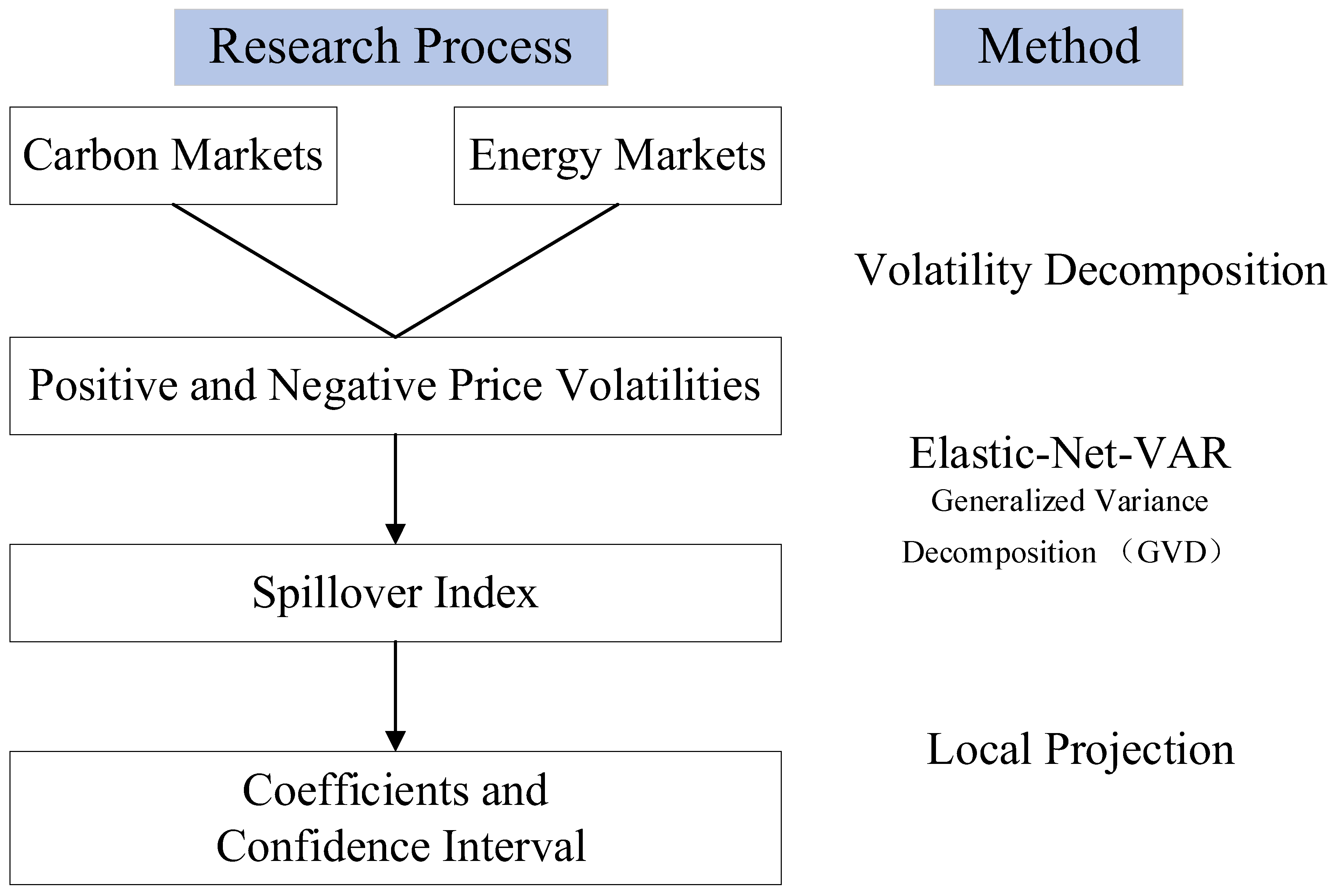
4. Methods and Data Description

4.1. Realized Semi-Variance

Barndorff-Nielsen et al. (2008) [6] proposed Realized Semi-variance (RS) and divided it into rising realized semi-variance (RS+) and falling realized semi-variance (RS-) according to the positive and negative returns. With reference to Patton and Sheppard (2015) [39], we decompose the realized volatility of carbon prices and energy prices based on the direction of daily return, and the expression is as follows:

$$R{S}_{i,t}^{+}=\sum _{k=1}^{K_t}{r}_{i,tk}^{2}I\left(r_{i,tk}>0\right),R{S}_{i,t}^{-}=\sum _{k=1}^{K_t}{r}_{i,tk}^{2}I\left(r_{i,tk}<0\right),i=1,\cdots ,N;t=1,\cdots ,T$$

(6)

where, $R{S}_{i,t}^{+}$ is the positive volatility of market price on day $t$, $R{S}_{i,t}^{-}$ is the negative volatility of market price on day $t$; $r_{i,tk}$ is the daily rate of return of market $i$ on day $k$ of month $t$, $K_t$ is the number of days on day $t$, and $I(\cdot )$ is an indicative function.

Define the positive volatility sequence of $N$ markets at $t$ as $R{S}_t^{+}=(R{S}_{1,t}^{+},R{S}_{2,t}^{+},\cdots ,R{S}_{N,t}^{+}{)}^{\prime }$ and the negative volatility sequence as $R{S}_t^{-}=(R{S}_{1,t}^{-},R{S}_{2,t}^{-},\cdots ,R{S}_{N,t}^{-}{)}^{\prime }$. The volatility sequence of these $N$ markets at $t$ is composed of positive and negative volatility sequences, that is $R{S}_t=(R{S}_{1,t}^{+},R{S}_{2,t}^{+},\cdots R{S}_{N,t}^{+},R{S}_{1,t}^{-},R{S}_{2,t}^{-},\cdots R{S}_{N,t}^{-}{)}^{\prime }$.

4.2. Elastic-Net-VAR Model

Assume that the volatility sequence of $N$ markets follows the following VAR(p) process:

$$R{S}_t=\mu +\sum _{i=1}^p{\Phi }_{i}R{S}_{t-i}+{\epsilon }_t, t=1,\cdots ,T$$

(7)

$R{S}_t=(R{S}_{1,t}^{+},R{S}_{2,t}^{+},\cdots R{S}_{N,t}^{+},R{S}_{1,t}^{-},R{S}_{2,t}^{-},\cdots R{S}_{N,t}^{-}{)}^{\prime }$ is a $2N$ dimensional column vector; ${\Phi }_i$ is the $2N\times 2N$ dimensional coefficient matrix; $\mu$ is the $2N$ dimensional intercept column vector; ${\epsilon }_t~(0,\Sigma )$. The number of parameters to be estimated in Function (7) is ${\left(2N\right)}^2\times p+2N$. When the number of endogenous variables is too large, the VAR model will face the problem of a “dimensional curse”.

To solve the estimation problem of the high-dimensional VAR model, we adopted the Elastic-Net method for dimensionality reduction and estimation [12]. The elastic-net method is a combination of Ridge Regression and LASSO (Least Absolute Shrinkage and Selection Operator). Incorporating the advantages of both, its estimator can not only shrink and select but also has the oracle property.

The estimation expression of the elastic net method is shown in Equation (8):

$$\underset{\mu ,\Phi }{argmin}{\sum _{t=1}^T‖R{S}_t-\mu -\sum _{i=1}^p{\Phi }_{i}R{S}_{t-i}‖}_2^2+\lambda \left(\alpha {‖\Phi ‖}_1+\left(1-\alpha \right){‖\Phi ‖}_2^2\right)$$

(8)

For an $m\times n$ dimensional matrix A, ${‖A‖}_F={\left({\sum }_{i=1}^m{\sum }_{j=1}^n{\left|A_{ij}\right|}^F\right)}^{1/F}$ denotes F-norm ($F=\mathrm{1,2},\dots$) and $A_{ij}$ is the element of the row i and column j of the matrix A. $\Phi =\left[{\Phi }_1,\dots ,{\Phi }_p\right]$; $\lambda$ is the penalty parameter; $\alpha$ is the adjustment parameter; ${‖\Phi ‖}_1$ is the penalty term of LASSO; ${‖\Phi ‖}_2^2$ is the penalty term of ridge regression. When $\alpha =0$, the elastic network degenerates into ridge regression; When $\alpha =1$, the elastic network degenerates to LASSO; When $0<\alpha <1$, elastic-net is a compromise between ridge regression and LASSO. The penalty parameter $\lambda$ determines the degree of compression of the parameter. We select $\lambda$ optimally by Rolling Cross-Validation. Referring to the study of Demirer et al. (2018) [12], we set the adjustment parameter $\alpha$ to 0.5.

4.3. Spillover Effect Analysis Based on Elastic-Net-VAR Model

When the Elastic-Net-VAR model of Equation (8) satisfies the stability condition, it can be transformed into the form of an infinite order vector moving average $\mathrm{VMA}\left(\mathrm{\infty }\right)$: $R{S}_t={\sum }_{i=0}^{\mathrm{\infty }}{\Psi }_i{\epsilon }_{t-i}$. The coefficient matrix ${\Psi }_i$ follows the following recursive expression: ${\Psi }_i={\sum }_{j=1}^p{\Phi }_j{\Psi }_{i-j}$. When $i$ < 0, ${\Psi }_i$= 0; ${\Psi }_0$ is the identity matrix.

Generalized Variance Decomposition (GVD) is used to construct a spillover index [11] to investigate the contagion of price fluctuations in carbon markets and energy markets. According to the GVD, the proportion of $H$-step prediction error variance of variable $i$ that can be explained by variable j is as follows:

$${\theta }_{ij}\left(H\right)=\frac{{\sigma }_{jj}^{-1}{\sum }_{h=0}^{H-1}(e_i^{\prime }{\Psi }_h\Sigma e_j{)}^2}{{\sum }_{h=0}^{H-1}\left(e_i^{\prime }{\Psi }_h\Sigma {\Psi }_h^{\prime }{e}_i\right)}, i,j=\mathrm{1,2},\dots 2N$$

(9)

where $\mathsf{\Sigma }$ is the variance–covariance matrix of ${\epsilon }_t$; ${\sigma }_{jj}$ is the j-th diagonal element of $\mathsf{\Sigma }$, ei and ej represent selected column vectors where the i-th and j-th elements are 1 and the other elements are 0, respectively. Since ${\sum }_{j=1}^{2N}{\theta }_{ij}\left(H\right)\ne 1$ in the GVD, Equation (4) can be normalized by row summing:

$${\tilde{\theta }}_{ij}\left(H\right)=\frac{{\theta }_{ij}\left(H\right)}{{\sum }_{j=1}^{2N}{\theta }_{ij}\left(H\right)}, i,j=\mathrm{1,2},\dots 2N$$

(10)

Now that ${\sum }_{j=1}^{2N}{\tilde{\theta }}_{ij}\left(H\right)=1$ and ${\sum }_{i,j=1}^{2N}{\tilde{\theta }}_{ij}\left(H\right)=2N$, ${\tilde{\theta }}_{ij}\left(H\right)$ can measure the influence level of variable j on variable $i$ during the prediction period $H$. The $2N\times 2N$-order matrix built with ${\tilde{\theta }}_{ij}\left(H\right)$ as elements can identify the spillover structure of positive and negative price volatilities in each carbon market and energy market, as shown in

Table 3. Spillover table for positive and negative price volatilities.

		$\mathit{R}{\mathit{S}}^{+}$				$\mathit{R}{\mathit{S}}^{-}$
		$\mathit{R}{\mathit{S}}_1^{+}$	$\mathit{R}{\mathit{S}}_2^{+}$	$\cdots$	$\mathit{R}{\mathit{S}}_{\mathit{N}}^{+}$	$\mathit{R}{\mathit{S}}_1^{-}$	$\mathit{R}{\mathit{S}}_2^{-}$	$\cdots$	$\mathit{R}{\mathit{S}}_{\mathit{N}}^{-}$
$R{S}^{+}$	$R{S}_1^{+}$	${\tilde{\theta }}_{1,1}$	${\tilde{\theta }}_{1,2}$	$\cdots$	${\tilde{\theta }}_{1,N}$	${\tilde{\theta }}_{1,N+1}$	${\tilde{\theta }}_{1,N+2}$	$\cdots$	${\tilde{\theta }}_{\mathrm{1,2}N}$
	$R{S}_2^{+}$	${\tilde{\theta }}_{2,1}$	${\tilde{\theta }}_{2,2}$	$\cdots$	${\tilde{\theta }}_{2,N}$	${\tilde{\theta }}_{2,N+1}$	${\tilde{\theta }}_{2,N+2}$	$\cdots$	${\tilde{\theta }}_{\mathrm{2,2}N}$
	$⋮$	$⋮$	$⋮$	$\ddots$	$⋮$	$⋮$	$⋮$	$\ddots$	$⋮$
	$R{S}_N^{+}$	${\tilde{\theta }}_{N,1}$	${\tilde{\theta }}_{N,2}$	$\cdots$	${\tilde{\theta }}_{N,N}$	${\tilde{\theta }}_{N,N+1}$	${\tilde{\theta }}_{N,N+2}$	$\cdots$	${\tilde{\theta }}_{N,2N}$
$R{S}^{-}$	$R{S}_1^{-}$	${\tilde{\theta }}_{N+\mathrm{1,1}}$	${\tilde{\theta }}_{N+\mathrm{1,2}}$	$\cdots$	${\tilde{\theta }}_{N+1,N}$	${\tilde{\theta }}_{N+1,N+1}$	${\tilde{\theta }}_{N+1,N+2}$	$\cdots$	${\tilde{\theta }}_{N+\mathrm{1,2}N}$
	$R{S}_2^{-}$	${\tilde{\theta }}_{N+\mathrm{2,1}}$	${\tilde{\theta }}_{N+\mathrm{2,2}}$	$\cdots$	${\tilde{\theta }}_{N+2,N}$	${\tilde{\theta }}_{N+2,N+1}$	${\tilde{\theta }}_{N+2,N+2}$	$\cdots$	${\tilde{\theta }}_{N+\mathrm{2,2}N}$
	$⋮$	$⋮$	$⋮$	$\ddots$	$⋮$	$⋮$	$⋮$	$\ddots$	$⋮$
	$R{S}_N^{-}$	${\tilde{\theta }}_{2N,1}$	${\tilde{\theta }}_{2N,2}$	$\cdots$	${\tilde{\theta }}_{2N,N}$	${\tilde{\theta }}_{2N,N+1}$	${\tilde{\theta }}_{2N,N+2}$	$\cdots$	${\tilde{\theta }}_{2N,2N}$

.

Based on Table 3, we construct the total volatility spillover index between carbon markets and energy markets:

$$TSI\left(H\right)=\frac{{\sum }_{\begin{array}{c}i,j=1\\ i\ne j,\left|i-j\right|\ne N\end{array}}^{2N}{\tilde{\theta }}_{ij}\left(H\right)}{2N}\times 100$$

(11)

The total volatility spillover index $TSI\left(H\right)$, which is the sum of the non-principal diagonal elements of the four parts in Table 1, is used to measure the overall level of volatility spillovers between markets. We further define the positive and negative price volatility spillover and inflow index at the system level in Appendix A.

4.4. Local Projection

We adopt the Local Projection method (Jordà, 2005) [15] to investigate the between carbon prices’ volatility and energy prices’ volatility interconnection:

$$\begin{array}{cc}{X_i}_{,t+h}={\alpha }_h+{\beta }_{h}COVI{D}_{G{R}_t}+{\gamma }_h{GPR}_{i,t}+{\mu }_{i,h}+{\epsilon }_{i,t+h},& h=\mathrm{0,1},\dots ,H\end{array}$$

(12)

where ${X_i}_{,t+h}$ is the spillover index we constructed before.${\alpha }_h$ represents the constant term, ${\mu }_{i,h}$ represents the individual fixed effect and ${\epsilon }_{i,t+h}$ represents the random disturbance term. We take the variables following Duan et al. (2021) [40] measuring COVID-19 cases—we use the 14-day moving average rate of confirmed COVID-19 cases to measure the severity of the pandemic. The specific construction method is as follows:

$$COVI{D}_{GR}=\frac{{\sum }_{t-13}^t\left[\mathit{ln}\left(1+\mathrm{Confirmed}\mathrm{Cas}{\mathrm{e}}_{j,t}\right)-\mathit{ln}\left(1+\mathrm{Confirmed}\mathrm{Cas}{\mathrm{e}}_{j,t-1}\right)\right]}{14};$$

($COVI{D}_{G{R}_t}$) and the Geopolitical Risk Index (GPR) (we downloaded it from https://www.matteoiacoviello.com/gpr.htm (accessed on 5 May 2023) ) calculated by Caldara and Iacoviello (2022) [41] as shock variables, and finally obtain the dynamic effects of COVID-19 and Geopolitical Risk to spillover index we constructed.

4.5. Data

For the carbon price data, we utilize representative carbon prices from three key regions: Europe, China, and America. Specifically, the Carbon Price is sourced from the Bloomberg database, where we access the Aggregate Real Carbon Price data for Europe, China, and America. The original data are provided by Monash University and C2Zero.

As for the energy price data, we rely on existing literature to inform our selection of fossil fuel prices [42], encompassing coal, crude oil, and natural gas. Considering trading liquidity, we choose the futures closing prices of active contracts for IPE Brent Crude Oil, IPE UK Natural Gas, and IPE Rotterdam Coal. The energy price data is obtained from the Wind database.

The selected sample period spans from 1 July 2013 to 31 May 2023, with a daily frequency of data. This comprehensive dataset allows for a thorough analysis of the interconnectedness between carbon and energy price volatilities over the specified time frame, providing valuable insights into the dynamics of these markets.

Table 4. Descriptive statistics of primary variables.

Data Type	Variable	Obs	Mean	Std. Dev.	Min	Max
Prices	Carbon_US(USD)	2588	13.57	4.178	8.868	23.84
	Carbon EU(USD)	2588	28.91	21.07	9.611	83.25
	Carbon CHN(USD)	2588	5.137	2.384	2.093	21.47
	IPE Rotterdam Coal(USD)	1831	99.71	77.3	38.55	459
	IPE Brent Crude Oil(USD)	2547	69.62	22.5	23	129.5
	IPE UK Natural Gas(USD)	2474	78.98	85.91	9.04	606.2
Shocks	GPR(Index)	72	77.13	22.88	46.86	167.3
	COVID_19(%)	72	0.856	3.655	0	29.47

presents descriptive statistics.

5. Results

5.1. Full Sample Static Spillover Analysis

We put the prices of three major energy markets and the carbon prices of three markets, including China, in the same system and construct an Elastic-Net-VAR model containing 12 series. Furthermore, we use the generalized variance decomposition to construct the spillover index to investigate the spillover effect of carbon market and energy market price volatilities and capture the difference under positive and negative price volatilities. The maximum possible lag order of the Elastic-Net-VAR model is set to 3, and the number of forecast error variance decomposition periods H is set to 48 (4 years).

According to the static information spillover table calculated by the Elastic-Net-VAR model of positive and negative volatilities of the carbon price and energy price calculated by the RS method, on the one hand, the three main energy markets form an internally interdependent and inseparable entity. As depicted in

Table 5. Static spillover table of positive and negative price volatilities (%).

		Positive Price Volatilities						Negative Price Volatilities
		Crude Oil	Coal	Natural Gas	Carbon_ EU	Carbon_ US	Carbon_ CHN	Crude oil	Coal	Natural Gas	Carbon_EU	Carbon_ US	Carbon_ CHN
Positive Price Volatilities	Crude oil		5.35	0.10	1.49	1.14	0.82		1.68	0.55	11.20	0.08	0.15
	Coal	6.27		0.93	5.66	1.24	0.10	2.53		14.09	12.06	0.03	0.01
	Natural Gas	0.28	1.80		0.64	0.12	0.96	0.09	0.92		0.36	1.46	0.07
	Carbon_ EU	4.82	11.02	0.26		0.64	0.73	6.05	4.83	5.28		2.42	0.22
	Carbon_ US	3.64	0.73	0.08	1.07		1.32	8.03	1.32	0.54	3.46		0.02
	Carbon_ CHN	0.30	0.32	0.56	0.65	0.76		0.69	0.54	1.76	0.49	0.02
Negative Price Volatilities	Crude oil		3.43	0.05	1.75	1.25	0.75		2.09	1.10	13.87	0.18	0.16
	Coal	3.22		0.24	1.57	1.32	0.26	2.98		12.63	5.47	0.07	0.04
	Natural Gas	0.66	10.91		3.11	1.17	1.11	0.88	8.56		5.66	1.38	0.10
	Carbon_ EU	9.20	13.68	0.28		0.63	0.25	11.90	5.03	6.23		0.31	0.07
	Carbon_ US	0.68	0.22	2.17	4.22		0.19	0.97	0.15	2.81	2.74		0.41
	Carbon_ CHN	0.29	0.13	0.34	1.06	0.01		0.48	0.23	0.75	0.25	0.27

, the connectedness within the energy market is remarkably high at 81.34%, surpassing the overall connectedness (23.83%). On the other hand, there exists a reciprocal feedback mechanism between carbon price and energy price. The combustion of energy generates CO₂ emissions. According to Section 3 and Figure 3, When carbon prices increase, there is a decrease in demand for energy. As we discussed in Section 3, the supply price elasticity of energy prices is low. That is, prices have little effect on supply in the energy market. So, from the demand side, reduced demand for energy subsequently leads to lower energy prices. Conversely, when economic performance improves, both demand for energy and demand for carbon emission rights rise concurrently. The surge in economic activity has led to a sharp rise in the demand for energy around the world. At the same time, the three major economies we selected have a greater demand for carbon trading. In this case, firms involved in production not only consume more energy but also intensify their need for additional carbon emission rights. Under these dual mechanisms’ influence, the connectedness between carbon market prices and energy market prices undergoes constant fluctuations.

Secondly, the total spillover levels of positive and negative price volatility are 39.3% and 42.61%, respectively, while the total inflow levels are 44.93% and 50.33%. The asymmetric impact of positive and negative price volatilities is not only manifested in their magnitudes but also in their transmission dynamics through spillovers according to the Formula (A1). On the one hand, negative price volatilities calculated by Formula (1) induce market instability and pessimistic expectations among participants, thereby accelerating risk transmission via intermarket correlation channels with a significant influence on other markets. Conversely, the market’s sensitivity to positive price volatilities calculated by Formula (1) is relatively low, leading to a suppression of information channel-mediated spillovers to some extent. On the other hand, negative price volatility reflects a more fragile market condition that renders it susceptible to spillovers from other markets. As economic conditions deteriorate further, the overall spillover effect across all markets tends to increase; however, the robust operational state exhibited by the market under positive price volatilities enhances its resilience and ability to withstand risks effectively. Consequently, compared with positive price volatilities, negative volatilities induce more intense risk resonance, resulting in higher levels of spillover.

Finally, the mutual spillover level between positive and negative price volatilities calculated by Formulas (A3) and (A4) is about 24.17%, while the respective internal spillover level of the two is 23.6%, indicating the need to investigate both the connectedness of price volatility in the same direction and that in different directions across markets. This underscores the importance of decomposing positive and negative price volatilities. On the one hand, markets with similar exposure tend to exhibit synchronous movements, amplifying price volatility resonance within major international energy and carbon markets. Additionally, under common macroeconomic policy impacts, market prices experience co-movements that promote convergence of trends. On the other hand, due to interdependencies between upstream and downstream sectors in carbon and energy markets, supply-demand mechanisms play a crucial role, leading to prominent instances of divergent movements. Overall, there exists a significant contagion effect of volatility risk between carbon and energy markets; notably, negative price volatilities exert a higher impact on the entire system compared to positive ones.

The directional spillover of positive and negative price volatility, as well as the relative spillover index for the six markets in the network according to Formula (A1) and Formula (A2), are presented in

Table 6. Directional spillovers and relative indices of positive and negative price volatilities (%).

Market	From+	From−	To+	To−	$\Delta$From	$\Delta$To
Crude oil	22.57	24.63	29.36	34.60	2.06	5.24
Coal	42.92	27.8	47.59	25.35	−15.12	−22.24
Natural gas	6.71	33.53	5.02	45.74	26.83	40.73
Carbon_EU	36.29	47.58	21.21	55.56	11.29	34.35
Carbon_US	20.2	14.55	8.29	6.22	−5.66	−2.07
Carbon_CHN	6.1	3.8	6.49	1.25	−2.29	−5.23

Note: + in table present positive volatilities and – present negative volatilities.

. In terms of spillover level, the coal market (47.59%), crude oil market (29.36%), and European carbon market (21.21%) rank highest among the six markets in terms of positive price volatility spillover, indicating that news that rises the price in these three markets will have a significant impact on other markets. Conversely, the European carbon market (55.56%), natural gas market (45.74%), and crude oil market (34.60%) exhibit the highest negative price volatility spillovers among all markets, suggesting that negative news from these three markets will strongly influence other markets. Coal is such an important ballast in energy that good news on coal prices is important to the industry. Although the positive price volatility spillover in the natural gas market is relatively limited, its negative price volatility spillover level ranks first among all energy markets. Compared with coal and crude oil, natural gas produces less pollution during mining and production. It does not require complex refining processes. As a result, natural gas is relatively clean as an energy source. Therefore, when the price of natural gas fluctuates negatively, more natural gas is used, which leads to a decline in the carbon price.

In terms of inflow level, the positive price volatilities of the coal market (42.92%), the European carbon market (36.29%), and the crude oil market (22.57%) are more prominently affected by other markets. The inflow level of negative price volatilities in the European carbon market (47.58%), the natural gas market (33.53%), and the coal market (27.8%) is higher than that in other markets, ranking the top three. The European carbon market has been established for a long time and has a more mature development and better liquidity. It has a closer relationship with the energy market, resulting in a higher level of inflow. In contrast, both the spillover level and inflow level of price volatilities in China’s carbon market are relatively low, indicating that it plays little role in the network composed of carbon markets and energy markets. This is because China’s carbon market is still under development and its market price is not enough to reflect the impact on the markets.

We further construct the relative spillover index of positive and negative price volatilities to reveal the difference in directional spillover of market prices according to Formula (A5). Table 6 shows that, first, there is a clear difference in the spillover level between positive and negative price volatility in each market. The excess value of positive and negative price volatilities in crude oil (5.24%), natural gas (40.73%) and European carbon market (34.35%) is significantly greater than 0, which indicates that compared with positive price volatilities, the volatility of negative price is more easily transmitted to other markets. The coal market (−22.24%), the US carbon market (−2.07%), and China’s carbon market (−5.23) show that the spillover effect of positive price volatilities is more prominent. Second, the direction of price volatility has less impact on price volatility inflows than spillovers. Except for the US carbon market, the spillover level of positive and negative price fluctuations is generally higher than the inflow difference in the remaining markets. Among them, the spillover difference between positive and negative price volatilities in the natural gas market (26.83%), the European carbon market (11.29%) and the crude oil market (2.06%) are significantly greater than 0, which indicates that negative price volatilities will lead them into a vulnerable situation and increase the possibility of being affected by price volatilities in other markets.

Compared to positive price volatilities, negative price volatilities exhibit higher levels of spillover and inflow in the natural gas market, the European carbon market, and the crude oil market. These findings are closely linked to the unique characteristics of these markets. Firstly, due to geographical constraints and high transportation costs, most international trade in natural gas occurs through pipelines or ships, resulting in a regionalized gas market with four independent pricing systems. The regional nature of this market makes it less risk-averse and more susceptible to negative shocks while limiting the transmission of positive price volatilities across regions. Secondly, although both negative and positive price volatilities impact the crude oil market, negative volatility has a greater influence compared to its positive counterpart. However, unlike the natural gas market, there is not much disparity between the impacts of negative and positive volatilities on this particular commodity’s market dynamics. Lastly, given its long-established presence with mature development and good liquidity, the European carbon market exhibits significantly higher levels of spillover compared to other selected carbon markets in this study. Consequently, it is more likely for this specific carbon market to exert an impact on or be influenced by other markets within its system. This is also consistent with the assumptions made in this paper. We believe that the energy market is a global market, while the carbon market is more traded within the region. The global market has the characteristics of wide influence and strong risk contagion. They are more likely to be the initiators of risk. The trading market within the region is more likely to passively become the recipient of risks, that is, to become the recipient of diversified risks in the global market. To sum up, apart from the risk contagion within the energy market and the carbon market, in general, the energy market is the initiator of the risk, while the carbon market is mainly the recipient of the risk.

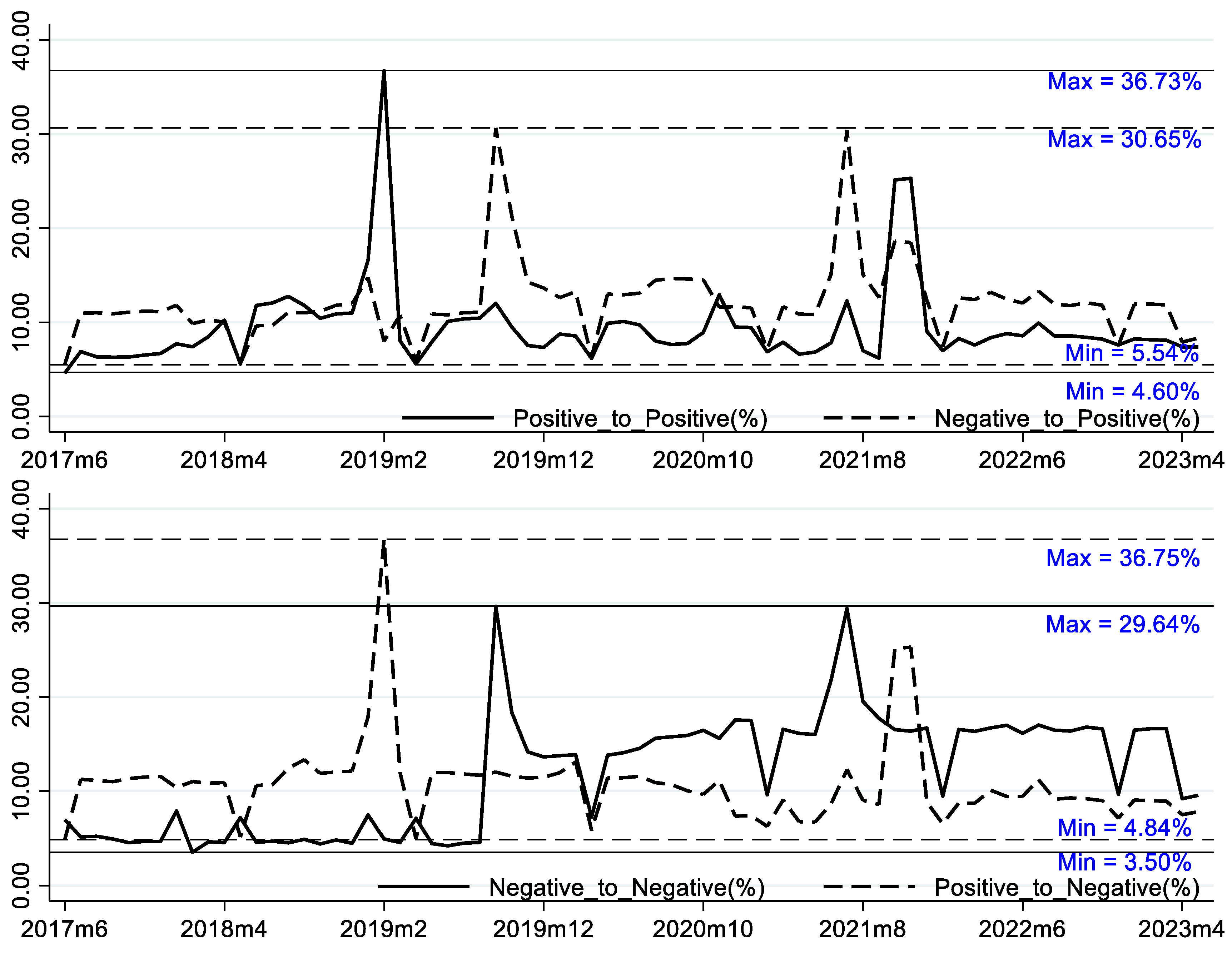
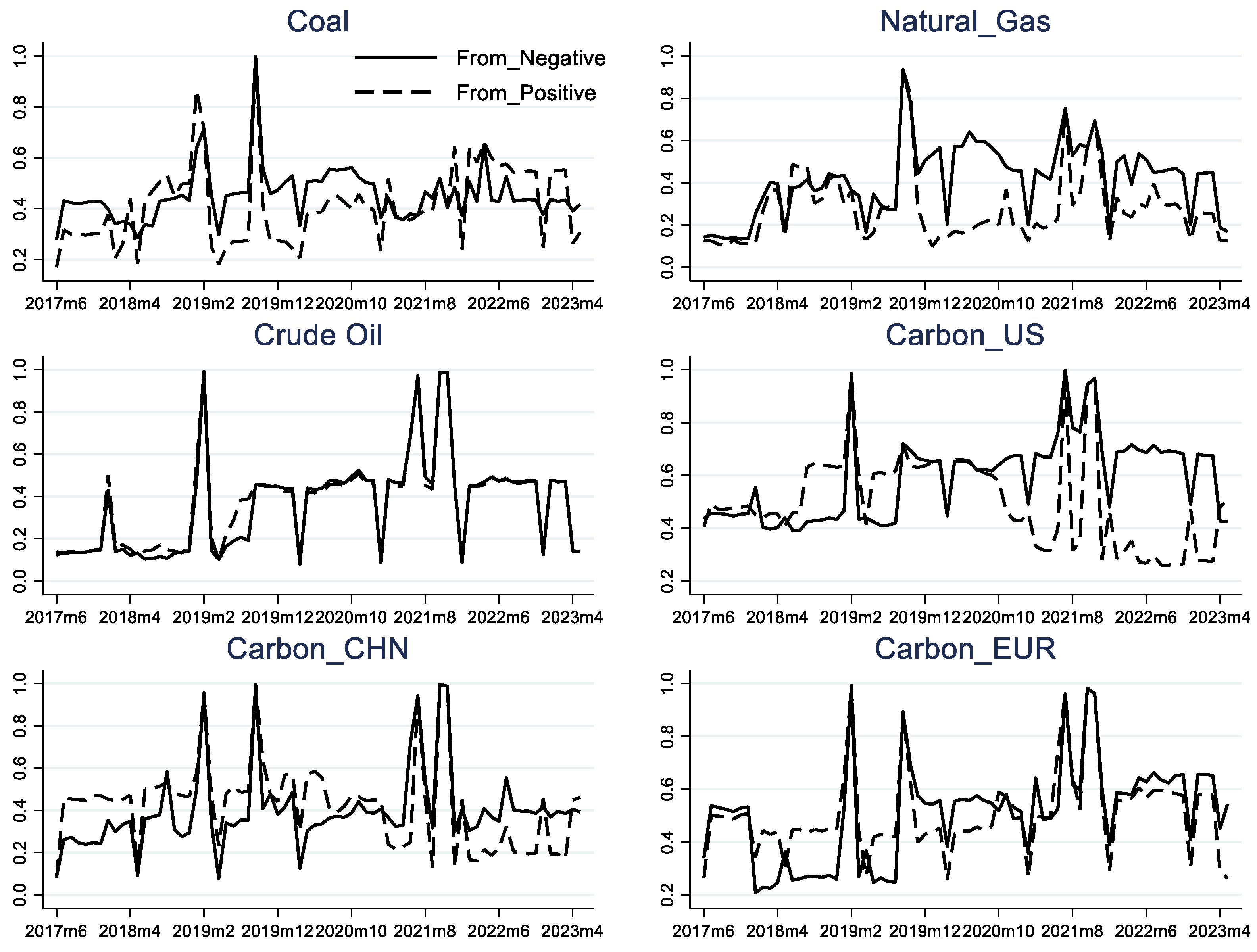
5.2. Dynamic Spillover Analysis of Rolling Samples

The static spillover analysis of the whole sample shows that there are differences in the total spillover and the directional spillover of each market. However, this analysis can only measure the average connectedness during the sample period, which means that it is difficult to capture the changes in the contagion of market price volatilities in different periods. Next, we set the rolling window to 48 months (four years) in the Elastic-Net-VAR, using the rolling spillover index to measure the price volatility spillover effect between markets and explore the difference between positive and negative price volatility spillover. Static network connectedness mainly reflects the average level of connectedness but does not include temporal information. Dynamic spillovers allow us to clearly observe the characteristics of connectedness in the time dimension.

Figure 4 shows the dynamic evolution characteristics of the total spillover network of the carbon price and energy price volatilities according to Formula (11). The total spillover index fluctuated in the range of 21.54–83.34%, with an average level of 43.46%. There is a significant price volatility contagion effect in the carbon markets and the energy markets. Figure 5 reveals the time series characteristics of spillover levels of positive and negative price volatility, respectively. In the whole sample period, the spillover level within positive price volatility is always higher than that from positive price volatility to negative price volatility. At the same time, the spillover level of negative price volatility to positive price volatility is significantly higher than the spillover level within negative price volatility. We can think of markets as more inclined to rise and fall together in response to shocks that raise prices; in a shock that lowers prices, markets tend to be more negatively correlated. We further find that the mean value of negative price volatility spillover is larger than that of positive price volatility, and the inflow of negative price volatility is smaller than that of positive price volatility. This is consistent with the research conclusion of the full sample, which again indicates that the spillover level of negative price fluctuations is higher and the inflow is lower; that is, negative price volatilities are more contagious.

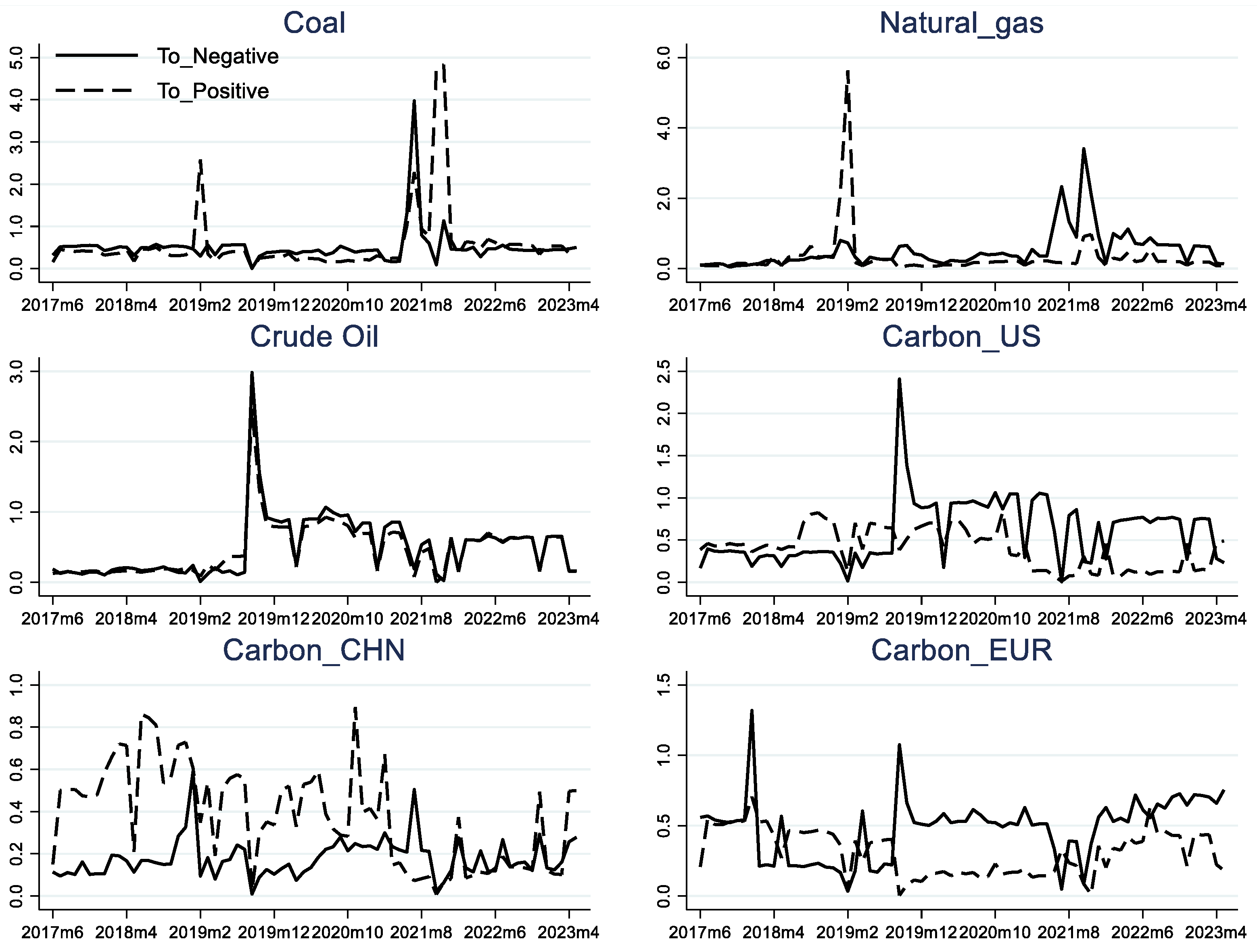
5.3. Directional Spillover Level

Since the relative index of positive and negative directional spillover of price volatility in the full-sample analysis cannot be significant, we further conduct a sample mean t-test on the spillover difference based on rolling analysis to reveal the directional asymmetry of price volatility spillover in each market.

The results of the mean t-test in

Table 7. Positive and negative price volatility spillover difference and mean test.

Spillover (%)	Negative Price Volatility		Positive Price Volatility		Difference	t-Statistic	p-Value
	Mean	Standard Error	Mean	Standard Error
Coal	51.02	5.31	56.88	9.57	−5.86	−0.53	0.30
Natural Gas	51.24	6.43	31.55	8.22	19.69	1.89	0.03
Crude oil	49.65	5.33	46.37	4.45	3.29	0.47	0.32
Carbon_US	59.85	4.52	39.89	2.76	19.96	3.77	0.00
Carbon_CHN	17.89	1.09	37.80	2.79	−19.91	−6.65	0.00
Carbon_EU	48.21	2.65	31.19	1.93	17.02	5.19	0.00

show that the spillover levels of positive and negative price volatilities in the coal market and the crude oil market are roughly the same, and the spillover difference is not significant at the level of 5%. In contrast, the spillover differences between positive and negative price volatility in the other four markets are all significant. On the one hand, the positive and negative price volatility excess of natural gas, US carbon price and EU carbon price is significantly greater than 0. This means that when they suffer from risk events that lead to price declines, the internal risks of the market will have a strong external contagion effect. On the other hand, the excess of positive and negative price fluctuations in China’s carbon market is significantly less than 0. This shows that the volatility spillover is greater when the price of China’s carbon market rises; that is, the positive news of China’s carbon market has a greater impact on the system of energy market and carbon market than the negative news. This is intuitive. As we discussed and analyzed earlier, carbon market trading is more confined to the domestic market. For the Chinese market, rising carbon market prices often mean an upward economic cycle and greater demand for carbon trading. As the second largest economy, its upturn in the economic cycle is indeed more likely to change global economic conditions and, through this, to transmit volatility to other markets. Therefore, we should pay close attention to the risk status of China’s carbon market and focus on preventing the volatility risk spillover induced by its rising price.

Table 8. Positive and negative price volatility inflow difference and mean test.

Inflow (%)	Negative Price Volatility		Positive Price Volatility		Difference	t-Statistic	p-Value
	Mean	Standard Error	Mean	Standard Error
Coal	45.33	1.22	41.41	1.88	3.93	1.75	0.04
Natural Gas	41.39	2.02	27.62	1.99	13.78	4.86	0.00
Crude oil	35.93	2.67	36.92	2.57	−0.99	−0.27	0.40
Carbon_US	58.98	1.82	49.98	2.09	9.00	3.24	0.00
Carbon_CHN	39.81	2.22	42.55	2.43	−2.74	−0.83	0.20
Carbon_EU	50.88	2.23	50.75	1.90	0.13	0.05	0.48

shows that the inflow difference between positive and negative price volatilities in the coal market, the natural gas market and the US carbon market is significantly positive at the 5% level. This shows that the market is more sensitive and vulnerable to the influence of other markets when the risk is high, that is, it is in the case of negative price volatilities. We further find that the spillover difference between positive and negative price volatility is the largest in the natural gas market. This is consistent with our exploration of natural gas market specificity in the full-sample static analysis. At the same time, this is consistent with our implicit assumptions. We can assume that the level of positive and negative price volatility in regional trading markets varies greatly. It should be noted that the fact that the difference is not significant does not mean that it is meaningless to study positive and negative price volatilities separately. In this case, positive and negative price volatility still have a difference and give us conditions under which we can study the specific impact path according to the difference in its positive and negative price volatility movements.

The mean directional spillover of positive and negative price volatility in Table 7 and Table 8 reflects the average level over the sample period. Figure 6 and Figure 7 further demonstrate the time-series variation of spillovers across markets calculated by Formula (A1) and Formula (A4). It can be seen that the spillover of positive and negative price volatility exhibits strong time variability. The difference between the spillover levels of positive and negative price volatility is much higher than the inflow level. Figure 6 reflects the asymmetry of spillover of positive and negative price volatilities, which has heterogeneous performance at different time points and in different markets. There is a shift in the dominance of positive and negative volatility at different stages. After the outbreak of COVID-19, spillovers in many markets are dominated by negative price volatilities. Combined with the actual situation, the sharp decline in crude oil prices during the COVID-19 pandemic has caused widespread contagion to the world economy. During the COVID-19 pandemic, the spillover level of positive price volatility and negative price volatility of crude oil both showed a significant upward trend. This further shows that extreme risk events will be transmitted to the whole system composed of carbon markets and energy markets through a certain market.

Figure 7 presents the time-series changes in the inflow levels of positive and negative volatility for each market. Firstly, inflows of negative price volatility dominate in both level and length of time. The inflow level of negative price volatility is higher than that of positive price volatility in almost all markets during the sample period at its peak. This reflects the weak ability of markets to resist risks in the downward stage of prices. Moreover, the strong sensitivity of the natural gas market and the three major carbon markets to the direction of price volatilities is not only limited to the mean level but also persists in time. Second, during the COVID-19 pandemic in 2019 and the following year, the inflow level of positive and negative price volatilities in most markets showed a significant upward trend, reflecting the common risk exposure mechanism we described above. Third, the global economy is still facing downward pressure in 2021. Except for the coal market, the inflow level of negative price volatility in other markets is significantly higher than that of positive price volatility. Only the crude oil market has comparable inflow levels of positive and negative price volatility. This has important implications for the global nature of the crude oil market as we noted earlier.

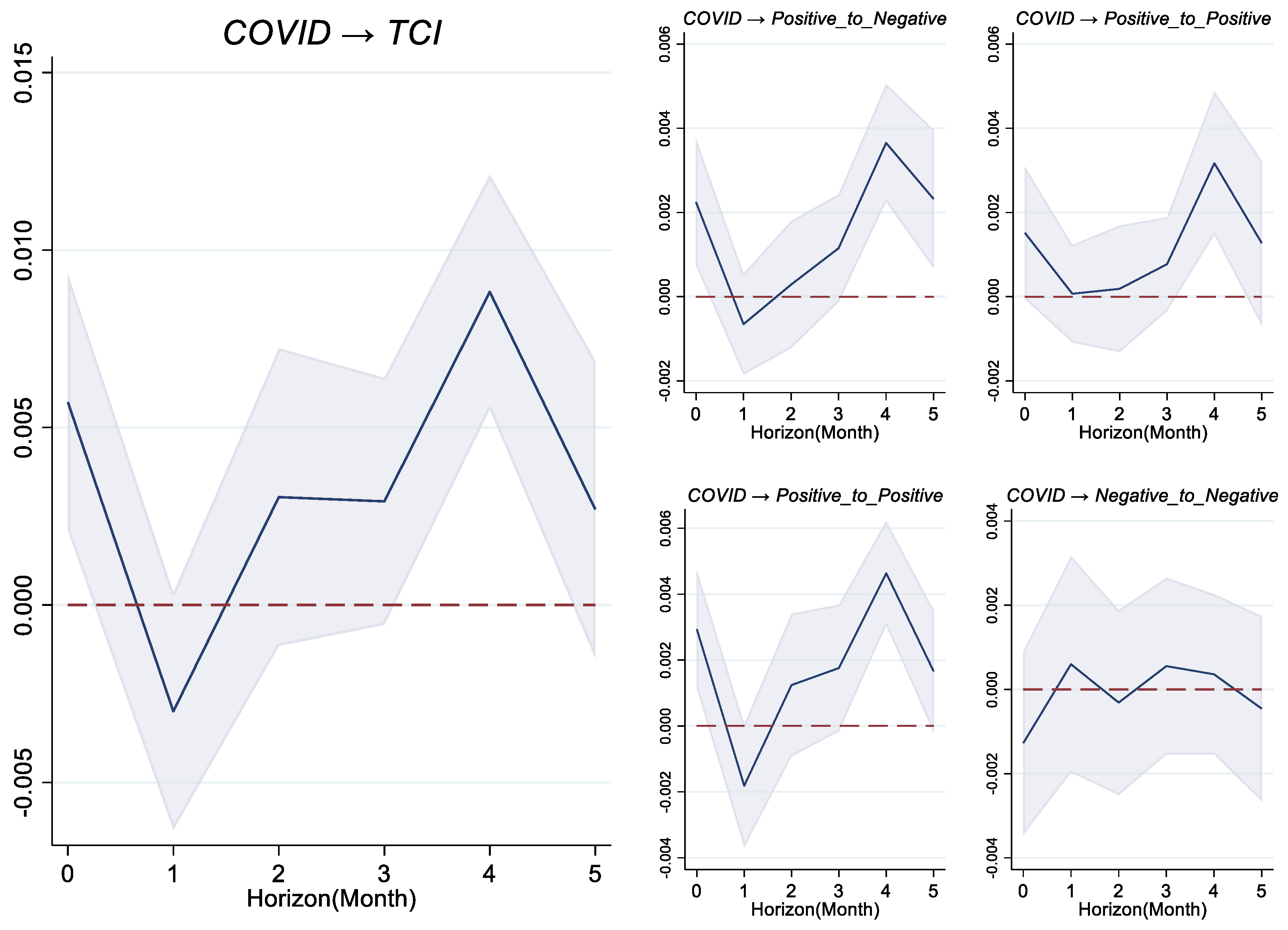
5.4. Testing the Impact of Shocks

To examine the impact of shocks on the spillover index, we use local projection (Jordà, 2005) [15] to explore whether shocks have impacts on the spillover of the network we constructed according to Formula (12).

Figure 8 shows that the COVID-19 pandemic has increased the overall connectedness of markets. This is consistent with the results of the previous study on positive and negative price volatility in each market. COVID-19, as a global public health event, has led to the same risk exposure of various markets and thus increased connectedness. As shown in Figure 8, the outbreak of COVID-19 led to a small increase in network connectedness, which reached a peak in the fourth month after that. This result proves that global shocks such as COVID-19 have a large and sustained impact on the connectedness between markets.

It shows that in addition to the impact of COVID-19 on the internal spillover of negative price volatility, it has increased the spillover between positive and negative price volatility and the spillover between positive price volatility in Figure 8. The COVID-19 pandemic has mainly increased the divergence between the carbon market price and the energy market price. This is in line with the situation of the economic downturn proposed in the previous part of this paper.

Figure 9 shows that geopolitical risks significantly reduce the overall connectedness of the network. The rise in geopolitical risk may have shaken international markets, but some markets in the network have restrictions on regional trading (e.g., natural gas markets, national carbon markets). Therefore, under the influence of geopolitical risks, the decrease in transaction frequency between markets of various countries leads to the decline of the overall connectedness of the network.

It shows that geopolitical risk only increases the transmission of positive price volatilities to positive price volatilities, while the other three kinds of connectedness all show a downward trend in Figure 9. Geopolitical risks mainly reduce the overall relevance of the network by reducing the contagion of negative price volatilities. Interestingly, geopolitical risk increases the transmission of positive price volatility to positive price volatility. This shows that rising prices in one market caused by geopolitical risks are more likely to affect other markets. But overall, because geopolitical risks did lead to a decline in the closeness of countries, the overall network connectedness declined.

6. Discussion

We utilize data from major international energy markets and carbon markets to calculate market volatility, both positive and negative, and construct a dynamic price volatility spillover network. Additionally, the local projection method is employed to examine the impact of shocks on price volatility spillover and analyze the underlying mechanism.

By considering extreme risk events’ influence on the network, several conclusions can be drawn. Firstly, constructing separate networks for positive and negative volatility reveals differences in price volatility connectedness. This highlights the significance of dividing market volatility into its positive and negative components for analyzing risk spillover. Moreover, it demonstrates that each market’s positive and negative volatilities are influenced by distinct mechanisms. Secondly, there exists a Connectedness mechanism between carbon prices and energy prices whereby an increase in energy demand leads to rising energy prices while negatively correlating with carbon prices; conversely, when energy supply drives down energy prices. Furthermore, both markets exhibit their own unique price volatility characteristics, resulting in varying properties of inter-market contagion at different stages. Lastly, the connectedness between carbon emission trading markets and energy markets is indeed affected by common risk exposure mechanisms such as public health events. The spillover effects and inflow of negative price volatilities are more pronounced compared to those of positive price volatilities. This is attributed to the fact that declining prices often indicate a market downturn, leading to the easy dissemination of adverse news across interconnected markets. Concurrently, increasing fragility diminishes its resilience against risks.

Compared to the existing literature, we do draw some interesting conclusions. First of all, we find that negative price volatilities often reflect the fragility of the markets, which provides a reference for risk-averse investors. In fact, the literature has focused on the impact of economic volatility when energy prices are used as a source of shock. The literature shows that rising and falling energy prices have asymmetric effects on the economy [43,44]. Combined with our results, we can see that news that causes prices to fall in various markets actually increases market vulnerability. We can, therefore, infer that when both energy and carbon prices fall, the economy tends to be in a more sluggish cycle and, therefore, is less resilient to risk.

Second, we found that the rise in geopolitical risk has led to a decline in the connectedness of the networks we have built. This is consistent with the existing literature but not exactly the same. The consistency is that we validate the important role of geopolitical risk in energy and carbon prices. The difference is that, according to our results, rising geopolitical risks reduce the overall correlation between energy prices and carbon prices. This is quite different from the paper we refer to. Lau et al. (2023) [45] used the volatility spillover approach of Diebold–Yilmaz to build a network of geopolitical risk, energy price and carbon price. It also explores the changes in network structure in the long, medium, and short term and argues that total connectedness is positive and effective in different periods. Indeed, our results suggest that rising geopolitical risk reduces the total connectedness index. It has to do with geographical dispersion. This further provides investors with channels to diversify risk across borders.

The research in this paper is useful to policymakers in several possible ways. First, the development of carbon markets is important to protect against risks from energy markets. According to our conclusions, carbon markets often act as recipients of energy risk. We believe that this may be due to the fact that the carbon market is not yet well developed and has not yet formed a limited risk mitigation mechanism. Taking China’s carbon market as an example, we can see that its net risk inflow is much higher than its net risk spillover. Both the positive volatility risk inflow and negative volatility risk inflow are at a high level. Therefore, accelerating the construction of carbon markets plays an important role in improving the ability of carbon markets to resist risks. Second, policy should be more committed to preventing the risks that cause prices to fall. As discussed in this paper, the contagion effect of negative price volatilities is greater than that of positive price volatilities. This means that shocks that cause price falls are more easily transmitted through the system. Therefore, faced with the potential impact of price declines, policy should be adopted earlier to counter the risk. Third, for major shocks, the timeliness of policies is important. Take the shock of the COVID-19 pandemic, for example. It is difficult to predict such events. However, according to the results of this paper, the risk contagion level did not peak after the outbreak of the novel coronavirus but peaked after a certain period of time. Therefore, in the face of unpredictable shocks, it is of great significance to take timely measures to strengthen the market’s ability to resist risks to mitigate the transmission of risks within the network.

Studies have diverged on the direction of the correlation between carbon prices and energy prices. In this paper, the positive price connectedness and negative price connectedness in each period are directly separated. But, this paper still has some shortcomings. In the future, we will further expand the research mainly from the following aspects. (1) Although this paper explores the correlation mechanism between carbon prices and energy prices based on positive and negative price volatilities, it fails to accurately analyze whether the connectedness changes are caused by supply shocks or demand shocks in each period. We will dig deeper into the fundamental information behind the connectedness of energy prices and carbon prices from the perspective of the macroeconomic cycle, which is of great significance for a comprehensive analysis of the connection mechanism between carbon prices and energy prices. (2) This paper is based on a global perspective and is expected to provide investors with global-based investment recommendations. However, due to data limitations and research focus, the number of countries selected in this paper is still small. In the future, we hope to build a more comprehensive global network to analyze the connectedness of global carbon and energy markets from a more open perspective.

References

1. Chevallier, J. A model of carbon price interactions with macroeconomic and energy dynamics. Energy Econ. 2011, 33, 1295–1312. [Google Scholar] [CrossRef]
2. Doda, B. Evidence on business cycles and CO2 emissions. J. Macroecon. 2014, 40, 214–227. [Google Scholar] [CrossRef]
3. Khan, H.; Metaxoglou, K.; Knittel, C.R.; Papineau, M. Carbon emissions and business cycles. J. Macroecon. 2019, 60, 1–19. [Google Scholar] [CrossRef]
4. Fan, J.; Zhang, X.; Wang, J.; Qian, D. Measuring the Impacts of International Trade on Carbon Emissions Intensity: A Global Value Chain Perspective. Emerg. Mark. Financ. Trade 2021, 57, 972–988. [Google Scholar] [CrossRef]
5. Glosten, L.R.; Jagannathan, R.; Runkle, D.E. On the Relation between the Expected Value and the Volatility of the Nominal Excess Return on Stocks. J. Financ. 1993, 48, 1779–1801. [Google Scholar] [CrossRef]
6. Barndorff-Nielsen, O.; Kinnebrock, S.; Shephard, N. Measuring Downside Risk-Realised Semivariance; 2008-W02; Department of Economics, University of Oxford: Oxford, UK, 2008. [Google Scholar]
7. Shahzad, S.J.H.; Naeem, M.A.; Peng, Z.; Bouri, E. Asymmetric volatility spillover among Chinese sectors during COVID-19. Int. Rev. Financ. Anal. 2021, 75, 101754. [Google Scholar] [CrossRef] [PubMed]
8. Bakas, D.; Triantafyllou, A. The impact of uncertainty shocks on the volatility of commodity prices. J. Int. Money Financ. 2018, 87, 96–111. [Google Scholar] [CrossRef]
9. Segal, G.; Shaliastovich, I.; Yaron, A. Good and bad uncertainty: Macroeconomic and financial market implications. J. Financ. Econ. 2015, 117, 369–397. [Google Scholar] [CrossRef]
10. Xu, W.; Ma, F.; Chen, W.; Zhang, B. Asymmetric volatility spillovers between oil and stock markets: Evidence from China and the United States. Energy Econ. 2019, 80, 310–320. [Google Scholar] [CrossRef]
11. Diebold, X.F.; Yılmaz, K. On the network topology of variance decompositions: Measuring the connectedness of financial firms. J. Econom. 2014, 182, 119–134. [Google Scholar] [CrossRef]
12. Demirer, M.; Diebold, F.X.; Liu, L.; Yilmaz, K. Estimating global bank network connectedness. J. Appl. Econom. 2018, 33, 1–15. [Google Scholar] [CrossRef]
13. Ma, R.; Liu, Z.; Zhai, P. Does economic policy uncertainty drive volatility spillovers in electricity markets: Time and frequency evidence. Energy Econ. 2022, 107, 105848. [Google Scholar] [CrossRef]
14. Balcilar, M.; Ozdemir, H.; Agan, B. Effects of COVID-19 on cryptocurrency and emerging market connectedness: Empirical evidence from quantile, frequency, and lasso networks. Phys. A Stat. Mech. Its Appl. 2022, 604, 127885. [Google Scholar] [CrossRef]
15. Jordà, Ò. Estimation and Inference of Impulse Responses by Local Projections. Am. Econ. Rev. 2005, 95, 161–182. [Google Scholar] [CrossRef]
16. Keppler, J.H.; Mansanet-Bataller, M. Causalities between CO2, electricity, and other energy variables during phase I and phase II of the EU ETS. Energy Policy 2010, 38, 3329–3341. [Google Scholar] [CrossRef]
17. Lutz, B.J.; Pigorsch, U.; Rotfuß, W. Nonlinearity in cap-and-trade systems: The EUA price and its fundamentals. Energy Econ. 2013, 40, 222–232. [Google Scholar] [CrossRef]
18. Aatola, P.; Ollikainen, M.; Toppinen, A. Price determination in the EU ETS market: Theory and econometric analysis with market fundamentals. Energy Econ. 2013, 36, 380–395. [Google Scholar] [CrossRef]
19. Zhang, Y.-J.; Sun, Y.-F. The dynamic volatility spillover between European carbon trading market and fossil energy market. J. Clean. Prod. 2016, 112, 2654–2663. [Google Scholar] [CrossRef]
20. Zhu, B.; Han, D.; Chevallier, J.; Wei, Y.-M. Dynamic multiscale interactions between European carbon and electricity markets during 2005–2016. Energy Policy 2017, 107, 309–322. [Google Scholar] [CrossRef]
21. Ji, Q.; Zhang, D.; Geng, J.-b. Information linkage, dynamic spillovers in prices and volatility between the carbon and energy markets. J. Clean. Prod. 2018, 198, 972–978. [Google Scholar] [CrossRef]
22. Batten, A.J.; Maddox, E.G.; Young, R.M. Does weather, or energy prices, affect carbon prices? Energy Econ. 2021, 96, 105016. [Google Scholar] [CrossRef]
23. Nazifi, F.; Milunovich, G. Measuring the Impact of Carbon Allowance Trading on Energy Prices. Energy Environ. 2010, 21, 367–383. [Google Scholar] [CrossRef]
24. Jin, Y.; Zhao, H.; Bu, L.; Zhang, D. Geopolitical risk, climate risk and energy markets: A dynamic spillover analysis. Int. Rev. Financ. Anal. 2023, 87, 102597. [Google Scholar] [CrossRef]
25. Liu, D.; Liu, X.; Guo, K.; Ji, Q.; Chang, Y. Spillover Effects among Electricity Prices, Traditional Energy Prices and Carbon Market under Climate Risk. Int. J. Environ. Res. Public Health 2023, 20, 1116. [Google Scholar] [CrossRef] [PubMed]
26. Meng, B.; Wei, B.; Yang, M.; Kuang, H. Measuring the time-frequency spillover effect among carbon markets and shipping energy markets: A global perspective. Energy Econ. 2023, 128, 107133. [Google Scholar] [CrossRef]
27. Naeem, M.A.; Arfaoui, N. Exploring downside risk dependence across energy markets: Electricity, conventional energy, carbon, and clean energy during episodes of market crises. Energy Econ. 2023, 127, 107082. [Google Scholar] [CrossRef]
28. Wang, T.; Wu, F.; Zhang, D.; Ji, Q. Energy market reforms in China and the time-varying connectedness of domestic and international markets. Energy Econ. 2023, 117, 106495. [Google Scholar] [CrossRef]
29. Hoque, M.E.; Soo-Wah, L.; Billah, M. Time-frequency connectedness and spillover among carbon, climate, and energy futures: Determinants and portfolio risk management implications. Energy Econ. 2023, 127, 107034. [Google Scholar] [CrossRef]
30. Naeem, M.A.; Peng, Z.; Suleman, M.T.; Nepal, R.; Shahzad, S.J.H. Time and frequency connectedness among oil shocks, electricity and clean energy markets. Energy Econ. 2020, 91, 104914. [Google Scholar] [CrossRef]
31. Girardi, G.; Tolga Ergün, A. Systemic risk measurement: Multivariate GARCH estimation of CoVaR. J. Bank. Amp; Financ. 2013, 37, 3169–3180. [Google Scholar] [CrossRef]
32. Xu, Y. Risk spillover from energy market uncertainties to the Chinese carbon market. Pac. -Basin Financ. J. 2021, 67, 101561. [Google Scholar] [CrossRef]
33. Dutta, A. Modeling and forecasting the volatility of carbon emission market: The role of outliers, time-varying jumps and oil price risk. J. Clean. Prod. 2018, 172, 2773–2781. [Google Scholar] [CrossRef]
34. Balcılar, M.; Demirer, R.; Hammoudeh, S.; Nguyen, D.K. Risk spillovers across the energy and carbon markets and hedging strategies for carbon risk. Energy Econ. 2016, 54, 159–172. [Google Scholar] [CrossRef]
35. Fleming, J.; Kirby, C.; Ostdiek, B. Information and volatility linkages in the stock, bond, and money markets. J. Financ. Econ. 1998, 49, 111–137. [Google Scholar] [CrossRef]
36. Kilian, L. Understanding the estimation of oil demand and oil supply elasticities. Energy Econ. 2022, 107, 105844. [Google Scholar] [CrossRef]
37. Gabaix, X.; Koijen, R.S. In Search of the Origins of Financial Fluctuations: The Inelastic Markets Hypothesis; National Bureau of Economic Research: Cambridge, MA, USA, 2021. [Google Scholar]
38. Caldara, D.; Cavallo, M.; Iacoviello, M. Oil price elasticities and oil price fluctuations. J. Monet. Econ. 2019, 103, 1–20. [Google Scholar] [CrossRef]
39. Patton, A.J.; Sheppard, K. Good Volatility, Bad Volatility: Signed Jumps and The Persistence of Volatility. Rev. Econ. Stat. 2015, 97, 683–697. [Google Scholar] [CrossRef]
40. Duan, Y.; El Ghoul, S.; Guedhami, O.; Li, H.; Li, X. Bank systemic risk around COVID-19: A cross-country analysis. J. Bank. Financ. 2021, 133, 106299. [Google Scholar] [CrossRef]
41. Caldara, D.; Iacoviello, M. Measuring geopolitical risk. Am. Econ. Rev. 2022, 112, 1194–1225. [Google Scholar] [CrossRef]
42. Duan, K.; Ren, X.; Shi, Y.; Mishra, T.; Yan, C. The marginal impacts of energy prices on carbon price variations: Evidence from a quantile-on-quantile approach. Energy Econ. 2021, 95, 105131. [Google Scholar] [CrossRef]
43. Hamilton, J.D. What is an oil shock? J. Econom. 2003, 113, 363–398. [Google Scholar] [CrossRef]
44. Cross, J.; Nguyen, B.H. Time varying macroeconomic effects of energy price shocks: A new measure for China. Energy Econ. 2018, 73, 146–160. [Google Scholar] [CrossRef]
45. Lau, C.K.; Soliman, A.M.; Albasu, J.; Gozgor, G. Dependence structures among geopolitical risks, energy prices, and carbon emissions prices. Resour. Policy 2023, 83, 103603. [Google Scholar] [CrossRef]
Figure 1. Volatility of Carbon Price and Energy Price.
Sustainability 16 05226 g001
Figure 2. Research framework.
Sustainability 16 05226 g002
Figure 3. Supply and Demand mechanism.
Sustainability 16 05226 g003
Figure 4. Time series characteristics of the total spillover level of price volatility.
Sustainability 16 05226 g004
Figure 5. Time series characteristics of spillover levels of positive and negative price volatility.
Sustainability 16 05226 g005
Figure 6. Time series characteristics of price volatility spillover in each market. Note: This graph shows the risk spillover levels of each major energy market and carbon market. To_Negative represents the spillover effect to other markets’ negative price volatilities. To_Positive represents the spillover effect to other markets’ positive price volatilities.
Sustainability 16 05226 g006
Figure 7. Time series characteristics of price volatility inflow in each market. Note: This graph shows the risk spillover levels of each major energy market and carbon market. From_Negative represents the inflow effect from other markets’ negative price volatilities. From_Positive represents the inflow effect from other markets’ positive price volatilities.
Sustainability 16 05226 g007
Figure 8. Effects of COVID-19 on the connectedness of price volatility. Note: The horizontal axis is the constant term of the local projection regression in months. The vertical axes correspond to the regression coefficients using local projection; The solid line is the regression coefficient of the connectedness index and the shock variable, and the shaded part is the 95% confidence interval of the regression coefficient. The blue line is regression coefficient for each period; The red line is Zero.
Sustainability 16 05226 g008
Figure 9. Effects of GPR on the connectedness of price volatility. Note: The horizontal axis is the constant term of the local projection regression in months. The vertical axes correspond to the regression coefficients using local projection; The solid line is the regression coefficient of the connectedness index and the shock variable, and the shaded part is the 95% confidence interval of the regression coefficient.
Sustainability 16 05226 g009